Some Fundamental Properties of a
Multivariate von Mises Distribution

Abstract

In application areas like bioinformatics multivariate distributions on angles are encountered which show significant clustering. One approach to statistical modelling of such situations is to use mixtures of unimodal distributions. In the literature (Mardia et al., 2011), the multivariate von Mises distribution, also known as the multivariate sine distribution, has been suggested for components of such models, but work in the area has been hampered by the fact that no good criteria for the von Mises distribution to be unimodal were available. In this article we study the question about when a multivariate von Mises distribution is unimodal. We give sufficient criteria for this to be the case and show examples of distributions with multiple modes when these criteria are violated. In addition, we propose a method to generate samples from the von Mises distribution in the case of high concentration.

1 Introduction

In biochemistry it is well known that the structure of macro-molecules such as proteins, DNA, and RNA can be described in terms of conformational angles. For proteins, these angles could be the dihedral and bond angles describing the conformation of the backbone together with additional angles for the configuration of the side chains (see e.g. Branden and Tooze, 1998). Data sets consist of the angles to describe each monomer in a macro-molecule, the number of angles required to give the conformation of a monomer determines the dimensionality of the problem. In non-coding RNA there can be 7 or 8 dihedral angles of importance per amino acid (Frellsen et al., 2009) and, if the side chains angles are included, many angles are required for amino acids in proteins (e.g. Harder et al., 2010). The resulting distributions on angles are multivariate, often highly structured, featuring various modes together with regions excluded by steric constraints (e.g. Mardia et al., 2011).

One way to approach the statistical modelling of such multimodal, multivariate distributions is to use mixture models with unimodal components. In the Euclidean space $\mathbb{R}^{p}$, an obvious choice for the components is to use normal distributions with appropriately chosen covariance matrices. For angular data, as considered in this article, the choice of component distribution in less clear, but a simple analogue of the multivariate normal distribution is the multivariate von Mises distribution (Mardia et al., 2008). This distribution is suggested for mixture modelling in Mardia et al. (2011). In order for a mixture model to be a useful description of a multimodal distribution, it is essential that the component distribution is unimodal. In case of the multivariate von Mises distribution, this constraint excludes some of the parameter range. Previous work has been complicated by the problem that no characterisation of the parameter values corresponding to the unimodal case was available. To solve this problem, this article provides sufficient criteria for the multivariate von Mises distribution to be unimodal and we show examples of distributions with multiple modes (where these criteria are violated). It should be noted that univariate circular distributions are well established (see, for example, Mardia and Jupp, 2000) but understanding of multicircular distributions is still evolving.

The multivariate von Mises distribution, first introduced in Mardia et al. (2008) and also known as the multivariate sine distribution, is denoted by $\mathrm{MVM}(\mu,\kappa,\Lambda)$. It is a distribution on the torus $\mathbb{T}^{p}=[0,2\pi)^{p}$ and is given by the density (w.r.t. the uniform distribution on angles)

$$\varphi(\theta;\mu,\kappa,\Lambda)=\frac{1}{Z(\kappa,\Lambda)}\exp\bigl{(}\kappa^{\top}c(\theta)+\frac{1}{2}s(\theta)^{\top}\Lambda s(\theta)\bigr{)}$$ (1)

for all $\theta\in\mathbb{T}^{p}$. Here $Z(\kappa,\Lambda)$ is the normalisation constant and we use the abbreviations

$$c_{i}(\theta)=\cos(\theta_{i}-\mu_{i}),\quad s_{i}(\theta)=\sin(\theta_{i}-\mu_{i})$$

for $i=1,\ldots,p$. The parameters of the distribution are the “mean” $\mu\in\mathbb{T}^{p}$, the “concentration parameter” $\kappa\in\mathbb{R}^{p}$ with $\kappa_{i}\geq 0$ for $i=1,\ldots,p$ and $\Lambda=(\lambda_{ij})\in\mathbb{R}^{p\times p}$ with $\Lambda^{\top}=\Lambda$ and $\lambda_{ii}=0$ for $i=1,\ldots,p$.

From the form of the density it is obvious that whenever $\kappa$ is “large” compared to $\Lambda$, the density will have exactly one maximum (where the vector $c(\theta)$ is approximately aligned with $\kappa$) and exactly one minimum (where $c(\theta)$ is approximately aligned with $-\kappa$). This effect is studied in section 2 where we give a sufficient criterion for the distribution to be unimodal. Conversely, for small $\kappa$ the quadratic term $s^{\top}(\theta)\Lambda s(\theta)$ in the density $\varphi$ dominates and one expects the occurrence of multimodal distributions. This situation is studied in section 3 where we show, by example, that a high number of modes is possible even in low dimensions. Finally, in section 4, we give an algorithm for generating samples of a $\mathrm{MVM}(\mu,\kappa,\Lambda)$ distribution for the unimodal case. This will be required as part of any algorithm to sample from a mixture model with $\mathrm{MVM}(\mu,\kappa,\Lambda)$ components.

2 High Concentration

In this section we derive a sufficient criterion for the $\mathrm{MVM}(\mu,\kappa,\Lambda)$ to be unimodal. Since the exponential function $\exp$ in the density (1) is strictly monotonically increasing and since the normalisation constant $Z(\kappa,\Lambda)$ does not depend on $\theta$, it suffices to consider the extrema of

$$f(\theta)=\kappa^{\top}c(\theta)+\frac{1}{2}s(\theta)^{\top}\Lambda s(\theta)$$ (2)

instead. These can be found by setting the partial derivatives

$$\partial_{i}f(\theta)=-\kappa_{i}s_{i}(\theta)+c_{i}(\theta)\sum_{k=1}^{p}\lambda_{ik}s_{k}(\theta)$$ (3)

equal to $0$: Since $\mathbb{T}^{p}$ is a compact, closed manifold, all local extrema of $f$ are located at $\theta\in\mathbb{T}^{p}$ with $\partial_{i}f(\theta)=0$ for $i=1,\ldots,p$, i.e. at critical points of $f$.

To characterise the critical points of $f$, we consider the second derivatives

$$\partial_{ij}f(\theta)=-\Bigl{(}\kappa_{i}c_{i}(\theta)+s_{i}(\theta)\sum_{k=1}^{p}\lambda_{ik}s_{k}(\theta)\Bigr{)}\delta_{ij}+c_{i}(\theta)\lambda_{ij}c_{j}(\theta)$$ (4)

where $\delta_{ij}$ denotes the Kronecker delta. If the Hessian matrix $H_{f}(\theta)=(\partial_{ij}f(\theta))_{i,j}$ at a critical point $\theta$ is negative definite, $\theta$ is a local maximum of $f$ and thus of $\varphi(\hbox to5.71527pt{\hss$\cdot$\hss};\mu,\kappa,\Lambda)$; if $H_{f}(\theta)$ is positive definite, $\theta$ is a local minimum; finally, if $H_{f}(\theta)$ has both positive and negative eigenvalues, the point $\theta$ is a saddle point.

For reference in the arguments below, we note that the biggest eigenvalue $\lambda_{\mathrm{max}}$ of a symmetric matrix $A=(a_{ij})\in\mathbb{R}^{p\times p}$ satisfies

$$\lambda_{\mathrm{max}}=\sup_{x\in\mathbb{R}^{p},|x|=1}x^{\top}Ax\geq\max_{i=1,\ldots,p}e_{i}^{\top}Ae_{i}=\max_{i=1,\ldots,p}a_{ii}$$

where $(e_{1},\ldots,e_{p})$ denotes the standard basis in $\mathbb{R}^{p}$. In particular, if the Hessian matrix at a critical point $\theta$ has a positive diagonal element, it has at least one positive eigenvalue and thus $\theta$ cannot be a local maximum. Similarly, the smallest eigenvalue $\lambda_{\rm min}$ satisfies $\lambda_{\rm min}\leq\min_{i=1,\ldots,p}a_{ii}$ and if $H_{f}(\theta)$ has a negative diagonal element, $\theta$ cannot be a local minimum.

Proposition 2.1.

Assume that the matrix

$$P=\operatorname{diag}(\kappa_{1},\ldots,\kappa_{p})-\Lambda$$

is positive definite. Then the global maximum of $\varphi=\varphi(\hbox to5.71527pt{\hss$\cdot$\hss};\mu,\kappa,\Lambda)$ is attained at $\theta=\mu$ and $\varphi$ has no other (local) maxima.

Proof 2.2.

For $\theta=\mu$ we get $\nabla f(\mu)=0$ and $H_{f}(\mu)=-P$; by assumption, this matrix is negative definite and thus $\theta=\mu$ is a local maximum. We now show that this is the only local, and thus the global, maximum of $f$.

Since $P$ is positive, the smallest eigenvalue $\lambda_{\rm min}$ of $P$ satisfies $0<\lambda_{\rm min}\leq\min_{i=1,\ldots,p}P_{ii}=\min_{i=1,\ldots,p}\kappa_{i}$ and thus we have $\kappa_{i}>0$ for $i=1,\ldots,p$. From equation (3) we see that $\partial_{i}f(\theta)=0$ implies $c_{i}\neq 0$ and consequently $\sum\lambda_{ik}s_{k}=\kappa_{i}s_{i}/c_{i}$. Substituting this into the expression for $\partial_{ij}f$ in (4) we find that the Hessian matrix $H_{f}$ at a critical point has the elements

$$\partial_{ij}f(\theta)=-\kappa_{i}\bigl{(}x_{i}+\frac{s_{i}^{2}}{c_{i}}\bigr{)}\delta_{ij}+c_{i}\lambda_{ij}c_{j}=-\frac{\kappa_{i}}{c_{i}}\delta_{ij}+c_{i}\lambda_{ij}c_{j}$$

where we write $c$ for $c(\theta)$ and $s$ for $s(\theta)$ to improve readability. If a critical point $\theta$ has $c_{i}(\theta)<0$ for an index $i\in\{1,\ldots,p\}$, then $H_{f}(\theta)_{ii}=-\kappa_{i}/c_{i}>0$ and thus $\theta$ cannot be a local maximum. Therefore we can assume $c_{i}(\theta)>0$ for $i=1,\ldots,p$.

Using the notation

$$P(\theta)=\operatorname{diag}\bigl{(}\frac{\kappa_{1}}{c_{1}(\theta)},\ldots,\frac{\kappa_{p}}{c_{p}(\theta)}\bigr{)}-\Lambda$$ (5)

we can equivalently re-write the condition $\nabla f(\theta)=0$ as

$$P(\theta)s(\theta)=0.$$ (6)

Since

$$P(\theta)=P+\operatorname{diag}\bigl{(}\kappa_{1}(\frac{1}{c_{1}(\theta)}-1),\ldots,\kappa_{p}(\frac{1}{c_{p}(\theta)}-1)\bigr{)}$$

is the sum of two positive matrices, it is positive and in particular non-singular. Thus, the only solution of (6) is $s=0$ which implies that the maximum at $\theta=\mu$ is the only critical point with $c_{i}\geq 0$ for $i=1,\ldots,p$. This completes the proof.

From the proof of proposition 2.1 we see that, if $\theta=\mu$ is the global and thus a local maximum of $\varphi$, the matrix $P$ must be positive semi-definite, i.e. the positivity condition is almost equivalent to $\varphi$ having the global maximum at $\mu$. The following corollary gives a sufficient (but not necessary) condition for the statement to hold; the given condition is often easier to verify in practice. Coincidentally, this stronger condition allows to also identify the minima of the von Mises density $\varphi$.

Corollary 2.3.

Assume

$$\kappa_{i}>\sum_{j=1}^{p}|\lambda_{ij}|\qquad\mbox{for all $i=1,\ldots,p$.}$$ (7)

Then the global maximum of $\varphi=\varphi(\hbox to5.71527pt{\hss$\cdot$\hss};\mu,\kappa,\Lambda)$ is attained at $\theta=\mu$, the global minimum is at $\theta=(\mu_{1}+\pi,\ldots,\mu_{p}+\pi)$ and these two points are the only (local) extrema of $\varphi$.

Proof 2.4.

By the Gershgorin theorem (Horn and Johnson, 1985, Theorem 6.1.1), the eigenvalues of $P$ are contained in the union of the closed discs $B(\kappa_{i},r_{i})\subseteq\mathbb{C}$ with radii $r_{i}=\sum_{j\neq i}|-\lambda_{ij}|$ for $i=1,\ldots,p$. Since $P$ is symmetric, its eigenvalues are real and since we have $\kappa_{i}>\sum_{j}\bigl{|}\lambda_{ij}\bigr{|}=r_{i}$, all eigenvalues of $P$ are positive. Thus the condition of the proposition is satisfied and $\theta=0$ is the global maximum of $\varphi$.

Similarly, the eigenvalues of the matrix $P(\theta)$ from (5) are contained in the union of the closed discs $B\bigl{(}\kappa_{i}/c_{i}(\theta),r_{i}\bigr{)}\subseteq\mathbb{R}$ with radii $r_{i}=\sum_{j\neq i}|-\lambda_{ij}|$ for $i=1,\ldots,p$. Since we have

$$\bigl{|}\frac{\kappa_{i}}{c_{i}(\theta)}\bigr{|}\geq\kappa_{i}>\sum_{j}\bigl{|}\lambda_{ij}\bigr{|}=r_{i},$$

none of the discs contain $0$ and the matrix $P(\theta)$ cannot have 0 as an eigenvalue. This shows that all solutions of (6), i.e. the critical points of $f$, satisfy $s(\theta)=0$ and thus $c(\theta)\in\{-1,1\}^{p}$.

To classify the critical points, we consider the Hessian matrix $H_{f}=\bigl{(}\partial_{ij}f(\theta)\bigr{)}_{ij}$. Invoking the Gershgorin theorem again, the eigenvalues of $H_{f}$ are contained in the union of the closed discs with centres $\partial_{ii}f(\theta)$ and radii $\sum_{j\neq i}|\partial_{ij}f(\theta)|$ for $i=1,\ldots,p$. Using (4) we have

$$\bigl{|}\partial_{ii}f(\theta)\bigr{|}=\bigl{|}\kappa_{i}c_{i}(\theta)\bigr{|}=\bigl{|}\kappa_{i}\bigr{|}>\sum_{j}\bigl{|}\lambda_{ij}\bigr{|}=\sum_{j}\bigl{|}c_{i}(\theta)\lambda_{ij}c_{j}(\theta)\bigr{|}=\sum_{j\neq i}|\partial_{ij}f(\theta)|,$$

none of these discs contain $0$ and thus the circles corresponding to $i$ with $c_{i}=1$ and with $c_{i}=-1$ respectively form two disjoint groups. We can conclude that for each $i$ with $c_{i}=1$ the matrix $H_{f}$ has a negative eigenvalue and for each $i$ with $c_{i}=-1$ the Hessian has a positive eigenvalue. Consequently, $\theta=\mu$ is the only local maximum of $f$, $\theta=(\mu_{1}+\pi,\ldots,\mu_{p}+\pi)$ is the local minimum of $f$ and all other critical points are saddle points.

It is easy to see that the statements about the minimum in corollary 2.3 do not necessarily hold under the weaker assumption from proposition 2.1. For example, the matrix

$$\Lambda=\begin{pmatrix}0&-2&2\\ -2&0&2\\ 2&2&0\end{pmatrix}$$

has eigenvalues $-4$, $2$ and $2$. Thus, for $\kappa=(3,3,3)$ the matrix $P$ is positive (the eigenvalues are $1$, $1$ and $7$), and the assumption of proposition 2.1 is satisfied. On the other hand, the Hessian matrix of $f$ at $\theta=(\mu_{1}+\pi,\mu_{2}+\pi,\mu_{3}+\pi)$ is $H_{f}(\theta)=\operatorname{diag}(\kappa_{1},\kappa_{2},\kappa_{3})+\Lambda$ and, since this matrix is not positive semi-definite (the eigenvalues are $-1$, $5$ and $5$), the minimum of the distribution cannot be at $(\mu_{1}+\pi,\mu_{2}+\pi,\mu_{3}+\pi)$.

3 Low Concentration

In this section we consider the case of “small” $\kappa$. In this case the structure of the extrema of a $\mathrm{MVM}(\mu,\kappa,\Lambda)$ distribution is much more complicated than for the concentrated case. We illustrate some of the possible scenarios with the help of examples, starting with the boundary case $\kappa=(0,0,\ldots,0)$ and then considering small but non-zero $\kappa$.

The following lemma shows that for $\kappa=0$ the case of a single global maximum can never occur.

Lemma 3.1.

For $\kappa=0$, the following statements hold:

1. The density of the multivariate von Mises distribution $\mathrm{MVM}(\mu,0,\Lambda)$ takes its maximal value on the set $\{\frac{1}{2}\pi,\frac{3}{2}\pi\}^{p}\subseteq\mathbb{T}^{p}$, i.e.

   $$\sup_{\theta\in\mathbb{T}^{p}}\varphi(\theta;\mu,0,\Lambda)=\sup_{\theta\in\{\frac{1}{2}\pi,\frac{3}{2}\pi\}^{p}}\varphi(\theta;\mu,0,\Lambda).$$

2. If $\theta$ is a maximum, then so is $(\theta_{1}+\pi,\ldots,\theta_{p}+\pi)$. In particular the number of isolated maxima of $f$ is always even (and thus cannot be $1$).

Proof 3.2.

Without loss of generality, we can assume $\mu=0$. Let $\theta^{*}\in\mathbb{T}^{p}$ be a global maximum of $\varphi(\hbox to5.71527pt{\hss$\cdot$\hss};0,0,\Lambda)$. As in proposition 2.1, this is equivalent to $\theta^{*}$ being a maximum of the function $f$ from equation (2). Since we assume $\kappa=0$, the formula for $f$ simplifies to

$$f(\theta)=\frac{1}{2}s(\theta)^{\top}\Lambda s(\theta)$$ (8)

and the partial derivatives of $f$ are given by

$$\partial_{i}f(\theta)=c_{i}(\theta)\sum_{k=1}^{p}\lambda_{ik}s_{k}(\theta).$$ (9)

Let $i\in\{1,2,\ldots,p\}$. Since $\lambda_{ii}=0$, the value $\sum_{k=1}^{p}\lambda_{ik}s_{k}(\theta)$ does not depend on $\theta_{i}$ and thus $\theta_{i}\mapsto\partial_{i}f(\theta)$ can only change sign at the points $\theta_{i}=\frac{1}{2}\pi,\frac{3}{2}\pi$. Consequently, $\theta_{i}\mapsto f(\theta)$ changes monotonically between the values $\theta_{i}=\frac{1}{2}\pi,\frac{3}{2}\pi$. Defining $\theta^{+}$ and $\theta^{-}$ by $\theta^{+}_{i}=\frac{1}{2}\pi$, $\theta^{-}_{i}=\frac{3}{2}\pi$, and $\theta^{+}_{j}=\theta^{-}_{j}=\theta^{*}_{j}$ for $j\neq i$ this shows that one of the two inequalities $f(\theta^{+})\geq f(\theta^{*})\geq f(\theta^{-})$ and $f(\theta^{-})\geq f(\theta^{*})\geq f(\theta^{+})$ holds. Since $\theta^{*}$ is a global maximum of $f$, equality holds in the upper bound and thus either $\theta^{+}$ or $\theta^{-}$ is also a global maximum. By repeating this procedure for $i=1,2,\ldots,p$ we find a global maximum where each coordinate is in the set $\{\frac{1}{2}\pi,\frac{3}{2}\pi\}$. This completes the proof of the first statement.

The second statement is a direct consequence of the fact that the function $f$ from (8) is invariant under the map $\theta\mapsto\theta+(\pi,\ldots,\pi)$.

Lemma 3.3.

Let $\kappa=0$ and $\Lambda\neq 0$. Then every global maximum $\theta$ of $\varphi(\theta;\mu,0,\Lambda)$ satisfies $\|s(\theta)\|_{\infty}=1$.

Proof 3.4.

Since the trace of a matrix equals the sum of its eigenvalues and since $\Lambda$ is a non-zero matrix with zero trace, $\Lambda$ must have a strictly positive eigenvalue $\lambda$. Let $x$ be a corresponding eigenvalue with $\|x\|_{\infty}\leq 1$. Then we can find $\theta=(\theta_{1},\ldots,\theta_{p})$ with $\sin(\theta_{i})=x_{i}$ for $i=1,2,\ldots,p$. This vector $\theta$ satisfies

$$f(\theta)=\frac{1}{2}s(\theta)^{\top}\Lambda s(\theta)=\frac{\lambda}{2}s(\theta)^{\top}s(\theta)>0.$$

Consequently the maximal value of $f$ is strictly positive.

Now let $\theta\in\mathbb{T}^{p}$ with $f(\theta)>0$ and $\|s(\theta)\|_{\infty}<1$, i.e. $\bigl{|}s_{i}(\theta)\bigr{|}<1$ for all $i\in\{1,\ldots,p\}$. Let $c=1/\|s(\theta)\|_{\infty}>1$ and $\tilde{s}=cs(\theta)$. Since $\|\tilde{s}\|_{\infty}=1$, we can find $\tilde{\theta}\in\mathbb{T}^{p}$ with $\sin(\tilde{\theta}_{i})=\tilde{s}_{i}$ for $i=1,2,\ldots,p$. This point satisfies

$$f(\tilde{\theta})=\frac{1}{2}\tilde{s}^{\top}\Lambda\tilde{s}=c^{2}\frac{1}{2}s(\theta)^{\top}\Lambda s(\theta)>f(\theta).$$

Therefore, $\theta$ cannot have been a maximum of $f$.

Example 1 ($\kappa=0$, two isolated modes). Consider a $\mathrm{MVM}(\mu,0,\Lambda)$ distribution with

$$\Lambda=\begin{pmatrix}0&1.75&0.77\\ 1.75&0&0.06\\ 0.77&0.06&0\end{pmatrix}.$$

Since $\kappa=0$, lemma 3.3 applies and shows that all maxima of $\varphi(\hbox to5.71527pt{\hss$\cdot$\hss};\mu,0,\Lambda)$ correspond to $\theta$ where $s(\theta)$ lies on the surface of the cube $Q=[-1,1]^{3}$. Thus, we can find the local extrema of $f$ by first finding the local extrema of $g(s)=\frac{1}{2}s^{\top}\Lambda s$ on the surface of $Q$ and then identifying the corresponding values $\theta$. To aid with finding the maxima of $g$, figure 1 shows a plot of $g$ on the (unwrapped) surface of $Q$. In the figure, the top-most square corresponds to $s_{3}=+1$, the centre square to $s_{2}=-1$, the right-most square to $s_{1}=+1$ and so on. One can see that the distribution has two modes, corresponding to $s(\theta)=(-1,-1,-1)$ and $s(\theta)=(+1,+1,+1)$.

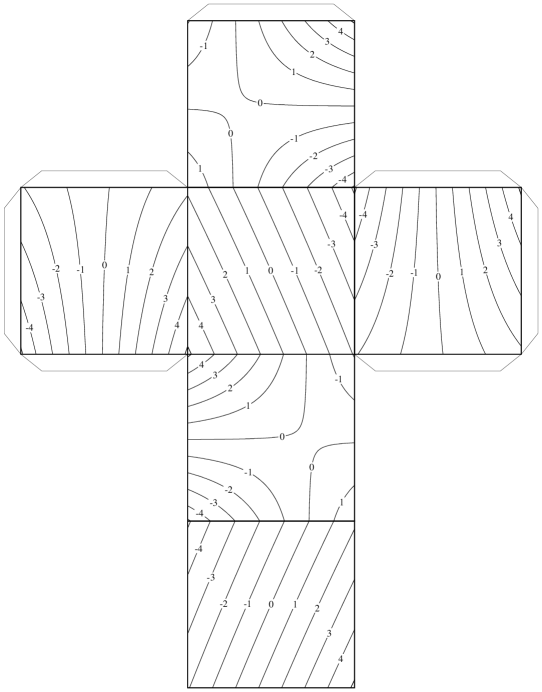
Figure 1: Visualisation of a von Mises density from example 1, as a function of $s(\theta)$ restricted to the surface of the cube $[0,1]^{3}$. The plot shows that the distribution has two modes.

Example 2 ($\kappa=0$, one extended mode). Consider a $\mathrm{MVM}(\mu,0,\Lambda)$ distribution with

$$\Lambda=\begin{pmatrix}0&-1&1\\ -1&0&1\\ 1&1&0\end{pmatrix}.$$

We can find the modes of this distribution in the same way as we did in example 1, the corresponding plot of $g$ is shown in figure 2. The figure shows that the density of this $\mathrm{MVM}(\mu,0,\Lambda)$ distribution has an extended maximum which forms a loop on the surface of the cube. Figure 2 shows the density as a function of $s(\theta)$. To give an idea of the distribution of the corresponding angles $\theta_{1},\theta_{2},\theta_{3}$ themselves, we show a scatter plot of a sample in figure 3. While this (much more conventional) diagram shows the distribution of the sample clearly, comparison with figure 2 makes it clear that the structure of the mode is difficult to understand from a scatter plot alone.

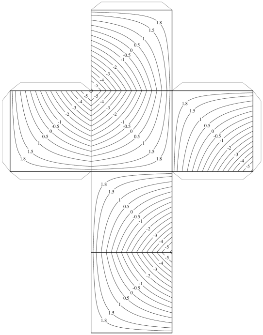
Figure 2: Visualisation of a von Mises density from example 2. One can see that the distribution has an extended maximum which loops around the cube in a “zig-zag belt”.

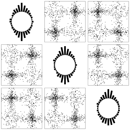
Figure 3: Scatter plot of 1000 samples from the distribution from example 2. To make the structure of the maximum more visible, the matrix $\Lambda$ was multiplied by 10, i.e. the plotted sample is from a $\mathrm{MVM}(0,0,10\,\Lambda)$ distribution. The regions where the scatter plots have higher intensity are not isolated modes of the distribution but are artefacts caused by the projection of $\mathbb{T}^{3}$ onto $\mathbb{T}^{2}$ where straight segments of the extended maximum are seen “head-on”.

The case of small, non-zero $\kappa$ can be seen as a perturbation of the case $\kappa=0$. Such a perturbation would normally just shift the extrema of the density around, but the following example shows that such a perturbation can also break a spatially extended maximum into a set of isolated maxima, thus increasing the number of modes.

Example 3 ($\kappa>0$, six isolated modes). The maximum of the von Mises distribution illustrated in figure 2 lives on a “ring” formed as the union of six lines in $\mathbb{T}^{3}$, aligned with the grid $\{\frac{1}{2}\pi,\frac{3}{2}\pi\}^{3}$. Since the $c_{i}$ are zero on the grid and take their maxima between the grid points, we would expect that adding a perturbation term $\kappa^{\top}c(\theta)$ with small $\kappa$ will not only shift these lines, but will also collapse this extended maximum into a collection of isolated maxima which live on the shifted lines, at the point where the perturbation was maximal. The following, explicit example gives a von Mises distribution in $\mathbb{T}^{3}$ with six isolated maxima.

Let $\eta>0$ and $\varepsilon=\sin(\eta)$. Define

$$\kappa=\begin{pmatrix}\varepsilon\\ \varepsilon\\ \varepsilon\end{pmatrix},\qquad\Lambda=\begin{pmatrix}0&-1&1\\ -1&0&1\\ 1&1&0\end{pmatrix}.$$

We will show that, for small enough $\eta$, the function $f(\theta)=\kappa^{\top}c(\theta)+\frac{1}{2}s(\theta)^{\top}\Lambda s(\theta)$ has local maxima at the six points $\theta^{1},\ldots,\theta^{6}\in\mathbb{T}^{3}$ given by the following table.

$$\begin{array}[]{c|ccc|ccc|ccc}\ell&\theta^{\ell}_{1}&\theta^{\ell}_{2}&\theta^{\ell}_{3}&s_{1}(\theta^{\ell})&s_{2}(\theta^{\ell})&s_{3}(\theta^{\ell})&c_{1}(\theta^{\ell})&c_{2}(\theta^{\ell})&c_{3}(\theta^{\ell})\\[6.45831pt] 1&0&\frac{3}{2}\pi+\eta&\frac{3}{2}\pi+\eta&0&-\sqrt{1-\varepsilon^{2}}&-\sqrt{1-\varepsilon^{2}}&1&\varepsilon&\varepsilon\\ 2&\frac{1}{2}\pi-\eta&\frac{3}{2}\pi+\eta&0&\sqrt{1-\varepsilon^{2}}&-\sqrt{1-\varepsilon^{2}}&0&\varepsilon&\varepsilon&1\\ 3&\frac{1}{2}\pi-\eta&0&\frac{1}{2}\pi-\eta&\sqrt{1-\varepsilon^{2}}&0&\sqrt{1-\varepsilon^{2}}&\varepsilon&1&\varepsilon\\ 4&0&\frac{1}{2}\pi-\eta&\frac{1}{2}\pi-\eta&0&\sqrt{1-\varepsilon^{2}}&\sqrt{1-\varepsilon^{2}}&1&\varepsilon&\varepsilon\\ 5&\frac{3}{2}\pi+\eta&\frac{1}{2}\pi-\eta&0&-\sqrt{1-\varepsilon^{2}}&\sqrt{1-\varepsilon^{2}}&0&\varepsilon&\varepsilon&1\\ 6&\frac{3}{2}\pi+\eta&0&\frac{3}{2}\pi+\eta&-\sqrt{1-\varepsilon^{2}}&0&-\sqrt{1-\varepsilon^{2}}&\varepsilon&1&\varepsilon\end{array}$$

For the convenience of the reader, the table also gives the vectors $s(\theta^{\ell})$ and $c(\theta^{\ell})$ for $\ell=1,\ldots,6$. By substituting these values into the formula for $\partial_{i}f$ from equation (3), it is easy to check that $\nabla f(\theta^{\ell})=0$ for $\ell=1,\ldots,6$ and thus all six points are critical points of $f$.

Substituting the values from the table into the formulas for $\partial_{ij}f$ from (4), we can compute the value of the Hessian matrix $H_{\ell}=H_{f}(\theta^{\ell})$ for $\ell=1,\ldots,6$. The results are as follows:

$$H_{1}=H_{4}=\begin{pmatrix}-\varepsilon&-\varepsilon&\varepsilon\\ -\varepsilon&-1&\varepsilon^{2}\\ \varepsilon&\varepsilon^{2}&-1\end{pmatrix},\quad H_{2}=H_{5}=\begin{pmatrix}-1&-\varepsilon^{2}&\varepsilon\\ -\varepsilon^{2}&-1&\varepsilon\\ \varepsilon&\varepsilon&-\varepsilon\end{pmatrix},\quad H_{3}=H_{6}=\begin{pmatrix}-1&-\varepsilon&\varepsilon^{2}\\ -\varepsilon&-\varepsilon&\varepsilon\\ \varepsilon^{2}&\varepsilon&-1\end{pmatrix}.$$

It can be checked that each of these matrices has eigenvalues $\lambda_{1}=-1+\mathcal{O}(\varepsilon^{2})$, $\lambda_{2}=-1+\mathcal{O}(\varepsilon^{2})$, and $\lambda_{3}=-\varepsilon+\mathcal{O}(\varepsilon^{2})$. Thus, for small enough $\varepsilon>0$, all six points are local maxima as required.

4 Sampling

In this section we discuss a simple method to generate samples from a $\mathrm{MVM}(\mu,\kappa,\Lambda)$ distribution, using the rejection sampling algorithm (Robert and Casella, 2004, Corollary 2.17). The method is restricted to small or moderate $p$, but works well for the case of high concentration. We assume that the matrix

$$P=\operatorname{diag}(\kappa_{1},\ldots,\kappa_{p})-\Lambda$$

is positive definite.

Without loss of generality we can assume $\mu=0$, the general case is then obtained by a simple shift. We denote the smallest eigenvalue of $P$ by $\lambda_{\rm min}>0$. The proposed algorithm uses independent angles $\theta_{1},\theta_{2},\ldots,\theta_{p}$ as proposals, distributed with density

$$g(\theta)=\prod_{i=1}^{p}\frac{\exp\bigl{(}\frac{\lambda_{\rm min}}{4}\cos(2\theta)\bigr{)}}{2\pi I_{0}\bigl{(}\frac{\lambda_{\rm min}}{4}\bigr{)}}.$$

This is the independent product of one-dimensional von Mises distributions, modified by replacing the angle $\theta$ by $2\theta$. Since we can efficiently generate samples $\tilde{\theta}_{i}$ from a one-dimensional von Mises distribution $\mathrm{VM}(0,\lambda_{\rm min}/4)$ (e.g. Best and Fisher, 1979), we can obtain samples from the density $g$ by taking $\theta_{i}=\tilde{\theta}/2$ with probability $1/2$ and $\theta_{i}=\tilde{\theta}/2+\pi$ else.

The target density is the density of the multivariate von Mises distribution $\mathrm{MVM}(0,\kappa,\Lambda)$, i.e. it is proportional to

$$f(\theta)=\exp\Bigl{(}\kappa^{\top}c(\theta)+\frac{1}{2}s(\theta)^{\top}\Lambda s(\theta)\Bigr{)}.$$

Using the inequalities $\cos(\theta)+\sin(\theta)^{2}/2\leq 1$ and $s(\theta)^{\top}Ps(\theta)\geq\lambda_{\rm min}s(\theta)^{\top}s(\theta)$, we find

$$f(\theta) =\exp\Bigl{(}\kappa^{\top}c(\theta)+\frac{1}{2}s(\theta)^{\top}\Lambda s(\theta)\Bigr{)}$$

$$=\exp\Bigl{(}\sum_{i=1}^{p}\kappa_{i}\bigl{(}c_{i}(\theta)+\frac{1}{2}s_{i}(\theta)^{2}\bigr{)}-\frac{1}{2}s(\theta)^{\top}Ps(\theta)\Bigr{)}$$

$$\leq\exp\Bigl{(}\sum_{i=1}^{p}\kappa_{i}-\frac{\lambda_{\rm min}}{2}s(\theta)^{\top}s(\theta)\Bigr{)}.$$

Finally, since $\cos(2x)=1-2\sin(x)^{2}$, we can rewrite this expression as

$$f(\theta) \leq\exp\Bigl{(}-\frac{p\lambda_{\rm min}}{4}+\sum_{i=1}^{p}\kappa_{i}\Bigr{)}\cdot\exp\bigl{(}\frac{\lambda_{\rm min}}{4}\sum_{i=1}^{p}c_{i}(\theta)\bigr{)}$$

$$=\exp\Bigl{(}-\frac{p\lambda_{\rm min}}{4}+\sum_{i=1}^{p}\kappa_{i}\Bigr{)}\cdot\bigl{(}2\pi I_{0}(\frac{\lambda_{\rm min}}{4})\bigr{)}^{p}\cdot g(\theta)$$

$$=:Cg(\theta).$$

Thus we have found a constant $C$ with $f\leq Cg$ and the rejection sampling algorithm can be applied.

In the rejection sampling algorithm, a proposal $\theta$ is accepted with probability $f(\theta)/Cg(\theta)$, i.e. with probability

$$p(\theta) =\frac{\exp\Bigl{(}\kappa^{\top}c(\theta)+\frac{1}{2}s(\theta)^{\top}\Lambda s(\theta)\Bigr{)}}{\exp\Bigl{(}\sum_{i=1}^{p}\kappa_{i}-\frac{\lambda_{\rm min}}{2}s(\theta)^{\top}s(\theta)\Bigr{)}}$$

$$=\exp\Bigl{(}\sum_{i=1}^{p}\kappa_{i}\bigl{(}c_{i}-1\bigr{)}+\frac{1}{2}s^{\top}(\Lambda+\lambda_{\rm min}I)s\Bigr{)}$$

where $I$ is the $p\times p$ identity matrix. Thus, the following algorithm can be used to generate samples of a $\mathrm{MVM}(\mu,\kappa,\Lambda)$ distribution when $P$ is positive:

1. Generate random variables

   $$\tilde{\theta}_{1},\ldots,\tilde{\theta}_{p}\sim\mathrm{VM}(0,\lambda_{\rm min}/4)$$

   $$\delta_{1},\ldots,\delta_{n}\quad\mbox{with $P(\delta_{i}=0)=P(\delta_{i}=\pi)=1/2$}$$

   $$U\sim\mathcal{U}\bigl{(}[0,1]\bigr{)},$$

   all independent of each other.

2. Let $s_{i}=\sin(\theta_{i})$ and $c_{i}=\cos(\theta_{i})$ for $i=1,2,\ldots,p$.

3. If the condition

   $$U\leq\exp\Bigl{(}\sum_{i=1}^{p}\kappa_{i}\bigl{(}c_{i}(\theta)-1\bigr{)}+\frac{1}{2}s(\theta)^{\top}(\Lambda+\lambda_{\rm min}I)s(\theta)\Bigr{)}$$

   is satisfied, output $\theta=(\theta_{1}+\mu_{1},\theta_{2}+\mu_{2},\ldots,\theta_{p}+\mu_{p})$ (i.e. the proposal is accepted).

4. Return to step 1.

We note that the algorithm still works when the eigenvalue $\lambda_{\rm min}$ is replaced by a lower bound $0<\hat{\lambda}_{\rm min}\leq\lambda_{\rm min}$ for the eigenvalues of $P$. This allows to apply the algorithm in situations where the eigenvalues of $P$ are not exactly known.

The efficiency of this algorithm is determined by its acceptance rate: If $Z$ is the normalisation constant which makes $\frac{1}{Z}f$ a probability density, then each proposal is accepted with probability $Z/C$. From Mardia et al. (2011, equation (3)) we know that, for high concentration, we have

$$Z\approx(2\pi)^{p/2}|P|^{-1/2}\exp\Bigl{(}\sum_{i=1}^{p}\kappa_{i}\Bigr{)}$$

where $|P|$ is the determinant of the matrix $P$. From Abramowitz and Stegun (1964, formula 9.7.1) we know

$$\sqrt{2\pi\kappa}\,\mathrm{e}^{-\kappa}I_{0}(\kappa)\longrightarrow 1$$

as $\kappa\to\infty$. Consequently, the asymptotic acceptance probability for high concentration is

$$\begin{split}\frac{Z}{C}&\approx\frac{(2\pi)^{p/2}|P|^{-1/2}\exp\bigl{(}\sum_{i=1}^{p}\kappa_{i}\bigr{)}}{\exp\bigl{(}-p\lambda_{\rm min}/4+\sum_{i=1}^{p}\kappa_{i}\bigr{)}\cdot(2\pi)^{p/2}(4/\lambda_{\rm min})^{p/2}\exp\bigl{(}p\lambda_{\rm min}/4\bigr{)}}\\ &=\frac{1}{2^{p}}\cdot\sqrt{\frac{\lambda_{\rm min}^{p}}{|P|}}.\end{split}$$ (10)

The proposed algorithm will be efficient if this probability is not to small. Considering the first factor on the right-hand side of (10), we see that the method only can be expected to perform well for sufficiently small values of $p$. The factor $1/2^{p}$ is expected, since the proposal distribution has $2^{p}$ modes, whereas the target distribution has only one. Since the determinant $|P|$ equals the product of all $p$ eigenvalues of $p$ (the smallest of which is $\lambda_{\rm min}$), the second factor on the right-hand side of (10) is big, if the eigenvalues of $P$ are all of the same magnitude, i.e. if the mode of the distribution is approximately rotationally symmetric.

Acknowledgements. The authors wish to thank John Kent for many helpful discussions.

References

Abramowitz and Stegun (1964)
M. Abramowitz and I. A. Stegun.
Handbook of Mathematical Functions.
Dover Publications, 1964.
Best and Fisher (1979)
D. J. Best and N. I. Fisher.
Efficient simulation of the von Mises distribution.
Journal of the Royal Statistical Society. Series C,
28(2):152–157, 1979.
URL http://www.jstor.org/stable/2346732.
Branden and Tooze (1998)
C. I. Branden and J. Tooze.
Introduction to Protein Structure.
Garland, second edition, 1998.
Frellsen et al. (2009)
J. Frellsen, I. Moltke, T. M., K. Mardia, J. Ferkinghoff-Borg, and
T. Hamelryck.
A probabilistic model of RNA conformational space.
PLoS Comput. Biol., 5(6), 2009.
10.1371/journal.pcbi.1000406.
Harder et al. (2010)
T. Harder, W. Boomsma, M. Paluszewski, J. Frellsen, K. Johansson, and
T. Hamelryck.
Beyond rotamers: a generative, probabilistic model of side chains in
proteins.
BMC Bioinformatics, 11(306), 2010.
10.1186/1471-2105-11-306.
Horn and Johnson (1985)
R. A. Horn and C. R. Johnson.
Matrix Analysis.
Cambridge University Press, 1985.
Mardia and Jupp (2000)
K. V. Mardia and P. E. Jupp.
Directional Statistics.
Wiley, 2000.
Mardia et al. (2008)
K. V. Mardia, G. Hughes, C. C. Taylor, and H. Singh.
A multivariate von Mises distribution with applications to
bioinformatics.
The Canadian Journal of Statistics, 36(1):99–109, 2008.
Mardia et al. (2011)
K. V. Mardia, J. T. Kent, Z. Zhang, C. Taylor, and T. Hamelryck.
Mixtures of concentrated multivariate sine distributions with
applications to bioinformatics.
Submitted, 2011.
Robert and Casella (2004)
C. P. Robert and G. Casella.
Monte Carlo statistical methods.
Springer Texts in Statistics. Springer, second edition, 2004.