Suzaku Observations of 4U 1957+11: Potentially the Most Rapidly Spinning Black Hole
in (the Halo of) the Galaxy

Abstract

We present three Suzaku observations of the black hole candidate 4U 1957+11 (V1408 Aql) — a source that exhibits some of the simplest and cleanest examples of soft, disk-dominated spectra. 4U 1957+11 also presents among the highest peak temperatures found from disk-dominated spectra. Such temperatures may be associated with rapid black hole spin. The 4U 1957+11 spectra also require a very low normalization, which can be explained by a combination of small inner disk radius and a large distance ($>10$ kpc) which places 4U 1957+11 well into the Galactic halo. We perform joint fits to the Suzaku spectra with both relativistic and Comptonized disk models. Assuming a low mass black hole and the nearest distance (3 $M_{\odot}$, 10 kpc), the dimensionless spin parameter $a^{*}\equiv Jc/GM^{2}\gtrsim 0.9$. Higher masses and farther distances yield $a^{*}\approx 1$. Similar conclusions are reached with Comptonization models; they imply a combination of small inner disk radii (or, equivalently, rapid spin) and large distance. Low spin cannot be recovered unless 4U 1957+11 is a low mass black hole that is at the unusually large distance of $\gtrsim 40$ kpc. We speculate whether the suggested maximal spin is related to how the system came to reside in the halo.

1. Introduction

4U 1957+11 is one of the few black hole candidates (BHC), like LMC X-1, LMC X-3, and Cyg X-1, that historically has been persistently active. In contrast to these other sources, however, it is a Low Mass X-ray Binary (LMXB; see Thorstensen, 1987; Hakala et al., 1999; Russell et al., 2010; Bayless et al., 2011). Also in contrast to other persistent Galactic BHC sources, 4U 1957+11 apparently has remained always in a spectrally soft state (Nowak et al., 2008). Its soft spectrum is well-modeled as a simple disk (Nowak & Wilms, 1999; Wijnands et al., 2002; Nowak et al., 2008; Dunn et al., 2010), i.e., a multi-temperature blackbody (Mitsuda et al., 1984) characterized by a peak temperature and a normalization related to the disk inner radius, inclination, and object distance. Approximately 15% of the over 40 pointed observations taken with the Rossi X-ray Timing Explorer (RXTE), however, also show a significant contribution (20–75% of the observed 3–18 keV flux) from a non-thermal/steep powerlaw component (Nowak et al., 2008; Dunn et al., 2010).

Optical observations suggest that we may be viewing the disk in 4U 1957+11 at a high inclination of $\sim 75^{\circ}$. Modulation over a 9.33 hr orbital period has ranged from $\pm 10\%$ and sinusoidal (Thorstensen, 1987) to $\pm 30\%$ and complex (Hakala et al., 1999). The latter has been interpreted as a high inclination warped disk being partly occulted by the secondary. On the other hand, Russell et al. (2010) failed to find any optical modulation over the orbital period, while Bayless et al. (2011) found nearly sinusoidal modulation. These latter authors attributed the optical modulation to illumination of the secondary, and noting a lack of any flattening at the lightcurve minimum, they modeled the system inclination with values as low as $20^{\circ}$ and not greater than $70^{\circ}$.

Currently, the mass, distance, and inclination of 4U 1957+11 are unknown. Based upon a comparison of the optical flux to the estimated optical luminosities of other BHC, however, Russell et al. (2010) have argued that 4U 1957+11 must lie at a distance $>20$ kpc. The possibility of a high inclination, however, makes such comparisons problematic. Russell et al. (2011) recently have presented near-simultaneous radio (Expanded Very Large Array – EVLA), optical (Faulkes Telescope North), and UV/X-ray (Swift) observations of 4U 1957+11. These observations show the soft state flux to be extremely quenched (factors of 330–810 times lower than the expected radio/X-ray flux ratio for hard state black hole sources), and demonstrate that the optical/UV flux are roughly consistent with the expectation of an irradiated disk. Those observations, however, do not definitively constrain the source’s inclination or distance. A minimum distance of $>5$ kpc; however, has been determined via high resolution X-ray spectroscopy. Ne ix $13.45$ Å absorption, associated with the warm/hot phase of the interstellar medium, is detected with a sufficient equivalent width to suggest that 4U 1957+11 resides above the galactic plane at this minimum distance or beyond (Yao et al., 2008; Nowak et al., 2008).

Nowak et al. (2008) showed that, with the exception of the $\approx 15$% of the time when a non-thermal component becomes prominent, disk models of the soft X-ray component have an approximately constant radius but a temperature that increases with flux (see Fig. 9 of Nowak et al. 2008). There is some indication for a slight increase in disk radius at the lowest flux levels, which was interpreted as possibly being associated with the source approaching a transition to a spectrally hard state. Such a transition is expected to occur at 2–3% $\mathrm{L_{Edd}}$, where $\mathrm{L_{Edd}}$ is the Eddington luminosity for the source in question (Maccarone, 2003). At the other extremes of flux in 4U 1957+11, the simple disk spectrum “drops out” (disk radius decreases in disk+powerlaw fits, or disk temperature decreases in disk+Compton corona fits) and is replaced by the non-thermal/steep powerlaw component (Nowak et al., 2008).

Although other persistent systems transiently show disk-dominated spectra, the persistent, soft spectra of 4U 1957+11 are perhaps the simplest and cleanest examples of “disk spectra”. XMM-Newton and Chandra observations show that there is very little absorption ($N_{\mathrm{H}}=1$–$2\times 10^{21}~{}\mathrm{cm^{-2}}$), while RXTE observations show that a hard tail contributes usually $<20\%$ of the flux. Furthermore, any additional components such as a broad Fe line (typically $<2\%$ peak residual in the fits) or a “smeared Fe edge” (which was never required or indicated in any of the RXTE spectra; Nowak et al. 2008) are very weak or absent. Thus the soft spectrum of 4U 1957+11 becomes the ideal testbed for modern disk atmosphere models that incorporate spin and other General Relativistic effects into their calculations (e.g., Li et al., 2005; Davis et al., 2005, 2006; Shafee et al., 2006).

Nowak et al. (2008) showed that the disk-fits to the XMM-Newton, Chandra, and RXTE spectra of 4U 1957+11 are characterized by a very low normalization, indicating some combination of large distance and low compact object mass, and very high inner disk temperature (1.3–1.8 keV). In other sources the latter has been associated with high black hole spin. To assess this possibility, Nowak et al. (2008) applied the relativistic disk model, kerrbb, of Li et al. (2005). The model parameters include a compact object mass and distance, disk inclination, accretion rate, spectral hardening factor (the ratio of color temperature to effective temperature), and dimensionless spin of the black hole, $a^{*}\equiv Jc/GM^{2}$. For a wide variety of masses and distances, fits to the XMM-Newton and Chandra spectra preferred maximal spin, $a^{*}\approx 1$. The RXTE spectra, in fact, could not be described with low spin, even when including a coronal or powerlaw component.

Various theoretical models of a disk atmosphere have suggested a spectral hardening factor of $\sim 1.7$. If this is correct, and utilizing the fact that the lowest flux observations must be $\mathrel{\hbox to0.0pt{\raise 2.20013pt\hbox{$>$}\hss}{\lower 2.20013pt\hbox{$\sim$}}}3\%\,\mathrm{L_{Edd}}$, then the spectral fits of 4U 1957+11 strongly suggest that it is a maximally spinning, $\approx$16 $M_{\odot}$ black hole at a distance of $\approx$22 kpc (Nowak et al., 2008). In this work we explore that claim with three recent Suzaku observations.

In Section 2 we describe the Suzaku observations and the details of the data processing. We then present the model fits to the resulting spectra in Section 3. Section 4 describes the scaling relations that we used to translate fits using a low mass, short distance black hole to comparably good fits involving a larger mass, further distance black hole. We then present our conclusions in Section 5.

Table 1Log of 4U 1957+11 Observations

Date		ObsID	Exposure
(yyyy-mm-dd)	(MJD)		(ksec)
2010-05-04	55320.82	405057010	35.80
2010-05-17	55333.80	405057020	37.20
2010-11-01	55502.19	405057030	15.50

Note. — Exposure times are after good time filtering, and represent the maximum exposure in an XIS detector when combining all data modes. MJD is the (non-barycenter corrected) average Modified Julian Date of the observation.

2. Observations and Data Analysis

The Suzaku data were reduced with tools from the HEASOFT v6.9 package and the calibration files current as of 2010 September. The instruments on Suzaku (Mitsuda et al., 2007) are the X-ray Imaging Spectrometer (XIS; Koyama et al., 2007) CCD detector covering the $\approx 0.3$–10 keV band, and the Hard X-ray Detector (HXD; Takahashi et al., 2007) comprised of the PIN diode detector (PIN) covering the $\approx 10$–70 keV band and the gadolinium silicate crystal detector (GSO) covering the $\approx~{}60$–600 keV band. The XIS had four separate detectors, XIS 0–3, with XIS 1 being a backside illuminated CCD. XIS 2 was lost due to a micrometeor hit in late 2006, and thus we only consider data from the remaining three XIS detectors. For all three observations described here, the hard X-ray fluxes were too low to lead to a significant detection in either of the HXD detectors, and therefore we do not include these data. A log of the observations is found in Table 1.

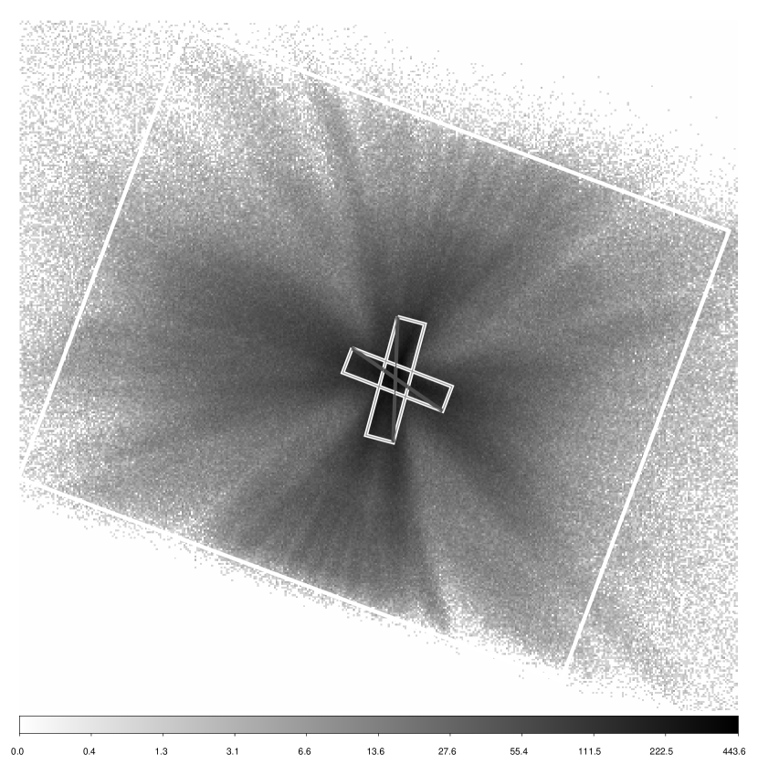
Figure 1.— The aspect corrected XIS 1 0.5–8 kev image on a logarithmic intensity scale from ObsID 405057010. The boxes outline the detector region from which the spectra were generated. The length of the short edge of the outer box is approximately $4^{\prime}.5$. The inner boxed regions with diagonal slashes were excluded from the spectra.

All of the XIS observations were run in a sub-array mode wherein 1/4 of the CCD was exposed with 2 second integration times. In preparing the XIS spectra, we first corrected each detector for Charge Transfer Inefficiency (CTI) using the xispi tool, and then reprocessed the data with xselect using the standard xisrepro selection criteria. Due to thermal flexing of the spacecraft, the attitude of the Suzaku spacecraft exhibits variability over the course of the observations and therefore the image of the source is not at a fixed position on the CCD. Standard processing reduces this variability and improves the Point Spread Function (PSF) image (Uchiyama et al., 2008); however, the standard tools do not yet fully correct the variable attitude induced blurring. We created an improved attitude reconstruction, and hence narrower PSF images, using the aeattcor.sl software described by Nowak et al. (2011). For the third observation, however, approximately half of the good time intervals (i.e., half of each spacecraft orbit) were affected by wobbles severe enough ($>1^{\prime}$) such that a large fraction of the image on the XIS 1 detector fell beyond the boundaries of the detector’s active regions. Although the images did not fall beyond the active region boundaries on the XIS 0 and XIS 3 detectors, there are serious questions about the accuracy of the generated response functions for such large off axis angles. We therefore excluded these times from the spectra, and reflect this in Table 1.

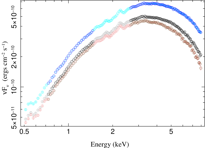
Figure 2.— The combined XIS 0, 1, and 3 spectra from each of the three Suzaku observations of 4U 1957+11, flux corrected with the detector responses. (ObsID 405057010 is the top spectrum, obsID 405057020 is the middle spectrum, and obsID 405057030 is the bottom spectrum.) The three observations share a common binning of approximately half width half maximum resolution of the detectors. Lighter colored data points represent energy bands that were ignored in the spectral fits described below.

Using the image generated from the improved attitude correction, we then used the pile_estimate.sl S-Lang script (Nowak et al., 2011) to estimate the degree of pileup in the XIS observations. For the spectra described in this work, the center of the PSF images were affected by as much as a 33% pileup fraction. We therefore exclude two, overlapping rectangular regions ($\approx 15\times 60$ pixels, nearly at right angles to one another) aligned along the brightest portions of the central PSF (see Fig. 1). We estimate that the remaining residual pileup fractions are $\lesssim 3\%$.

The outer limit of the extraction area was a rectangular region limited by the $4^{\prime}$ width of the 1/4 array boundaries. Additionally, we extracted background spectra from small rectangular regions, near the edges of the chips, that avoided as much as possible both the 4U 1957+11 image as well as the detector images of the on-board calibration sources. It is not entirely clear to what degree these regions are dominated by “true background”, as opposed to the wings of the PSF from the source. However, the normalized background flux remains at $<2\%$ of the source flux between 0.5–8 keV, and thus does not strongly affect the analyses presented in this work. The background flux starts to become an increasingly larger fraction of the source flux above 8 keV. For this reason, as well as due to any other uncertainties in the high energy calibration of the XIS detectors, we do not consider data above 8 keV.

Events in the XIS detectors were read out from either $3\times 3$ or $5\times 5$ pixel islands. We created individual spectra and response files for each detector and data mode combination. Little source variability was detected over the course of each observation, therefore the spectra were created for the full good time intervals represented by standard processing (excluding the times of very bad attitude errors, discussed above). Response matrices and effective area files were created with the xisrmfgen and xissimarfgen tools, respectively. For each observation, spectra for the different readout modes were combined during analysis on a chip-by-chip basis using the combine_datasets function within the Interactive Spectral Interpretation System (ISIS) fitting program (Houck & Denicola, 2000). That is, observations were kept separate, but within an observation all XIS 0 spectra were combined together, all XIS 1 spectra were combined, etc.

Although spectra for each observation and each XIS chip were kept separate, all spectra were jointly grouped on a common grid such that the XIS 0 spectra for the third (i.e., the faintest and shortest integration time) observation had a minimum combined signal-to-noise ratio of 5 in each energy bin ($\approx 25$ total counts in each bin, although the estimated background was included in the S/N criterion) and that the minimum number of channels per energy bin was at least the half width half maximum of the spectral resolution (see Nowak et al., 2011, for a further explanation of this criterion).

In Fig. 2 we present the flux corrected spectra, i.e., the counts spectra divided by the integrated response (see the ISIS user manual for a full description of this process). The spectra show strong deviations from a smooth continuum in the 1.5–2.6 keV region, near X-ray spectral features of Si and Ir. These systematic effects are seen in a wide variety of unrelated Suzaku spectra, hence our decision to exclude them from our fits. Likewise, there is a strong spectral feature near 0.55 keV, which we also suspect of being systematic in nature, hence our exclusion of data below 0.7 keV. To avoid these regions of poorly understood response, we only considered spectral energy ranges 0.7–1.5 keV and 2.6–8 keV. The smaller features near 0.75 keV and 0.9 keV are plausibly associated with Fe L, Ne K, and Ne ix absorption in the interstellar medium (ISM), as we discuss below.

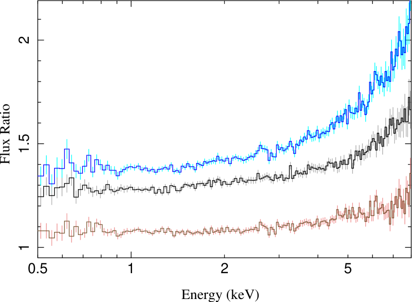
Figure 3.— Ratios of the flux corrected spectra shown in Fig. 2. The top ratio is observation 1/observation 3, the middle line is observation 1/observation2, and the bottom line is observation 2/observation 3.

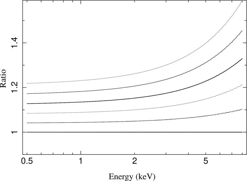
Figure 4.— Expectations for the flux ratio in a diskpn model when solely changing the peak temperature of the disk. The reference model has a 1.3 keV peak temperature. The peak temperature is varied in steps of 0.05 keV, up to 1.5 keV.

The suspected systematic features are relatively constant among the three observations, as is evident from the ratio of the flux corrected spectra as shown in Fig. 3. None of the systematic features are seen in these ratios. The ratios are relatively flat $\lesssim 2$ keV, and show a curve upward, with the degree of this curving being greatest for the ratio of the flux corrected spectra for the first and third observation. We discuss this further in the next section.

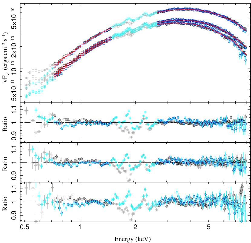
Figure 5.— The joint fit of an eqpair Comptonization model to the three spectra. The spectra share a common interstellar absorption column and a common normalization (i.e., disk inner radius), but have independent disk temperatures and coronal parameters. Black/grey spectra are the combined XIS 0 and 3 spectra, and blue/light blue are the XIS 1 spectra. Lightly shaded data were not included in the fit. The top residuals panel shows the ratio residuals for obsID 405057010, the middle residuals panel shows the ratio residuals for obsID 405057020, and the bottom panel shows the ratio residuals for obsID 405057030.

3. Spectral Fits

The spectral shape shown in Fig. 2, and the ratios seen in Fig. 3, are those expected for a disk-dominated spectrum wherein the flux changes are primarily dominated by variations of the peak temperature of the disk. We show the theoretical expectation for such a disk in Fig. 4. Here we use the diskpn model (Gierliński et al., 1999), which essentially is the spectrum from a Shakura-Sunyaev type disk (Shakura & Sunyaev, 1973) calculated using a simple pseudo-Netwonian potential and a no-torque boundary condition at the disk inner edge located at $6\,GM/c^{2}$. The flux goes to zero at the disk inner edge, and the disk temperature peaks at $\approx 10\,GMc^{2}$. This basic disk spectrum will underly the Comptonization fits discussed below.

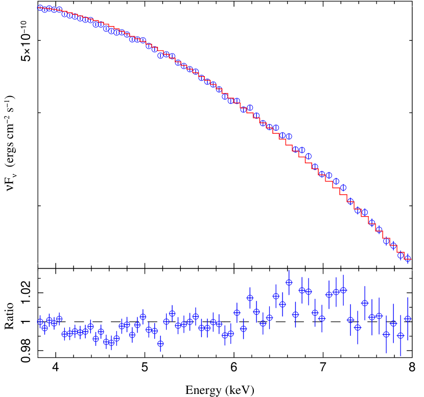
Figure 6.— A simultaneous fit to all three observations using the eqpair model, but excluding the broad Gaussian line in the Fe region. (The spectra were combined for the plot, but not the fits.

At energies approximately below the peak temperature, dominated by the Rayleigh-Jeans part of the thermal spectra, the ratios are fairly flat. At energies above the disk peak temperature, on the Wien tail of the thermal spectra, the ratios curve upward. There is a very good correspondence between the curves in Figs. 3 and 4. However, based upon our experience with RXTE spectra which extended out to $\approx 20$ keV, there is the possibility of additional spectral hardening beyond that associated with any rise in disk temperature. We therefore consider the eqpair Comptonization model (Coppi, 1999) which can use the diskpn as its input seed photon spectrum.

Table 2constant*TBnew*(eqpair+gaussian) Fits to 4U 1957+11 Spectra

ObsID	$N_{\mathrm{H}}$	$N_{\mathrm{eqp}}$	$kT_{\mathrm{disk}}$	$\ell_{\mathrm{h}}/\ell_{\mathrm{s}}$	$\tau_{\mathrm{net}}$	$N_{\gamma}$	$C_{\mathrm{xis0}}$	$C_{\mathrm{xis3}}$	0.7–8 keV Flux	$\chi^{2}/$DoF
	($10^{21}~{}\mathrm{cm^{-2}}$)	($10^{-4}$)	(keV)			($10^{-4}$)			($10^{-9}\,\mathrm{erg\,cm^{-2}\,s}$)
405057010	$0.200^{+0.001}_{-0.001}$	$1.926^{+0.001}_{-0.001}$	$1.477^{+0.001}_{-0.001}$	$0.37^{+0.03}_{-0.02}$	$0.017^{+0.002}_{-0.002}$	$1.4^{+0.4}_{-0.5}$	$1.019^{+0.002}_{-0.002}$	$1.020^{+0.002}_{-0.002}$	$1.09\pm 0.01$	1750.4/1014
405057020	$\cdots$	$\cdots$	$1.342^{+0.001}_{-0.001}$	$0.05^{+0.01}_{-0.01}$	$2.4^{+0.1}_{-0.1}$	$0.1^{+0.2}_{-0.1}$	$1.078^{+0.002}_{-0.002}$	$1.083^{+0.002}_{-0.002}$	$0.80\pm 0.04$	$\cdots$
405057030	$\cdots$	$\cdots$	$1.310^{+0.001}_{-0.001}$	$0.04^{+0.01}_{-0.01}$	$4.4^{+0.1}_{-0.1}$	$1.3^{+0.4}_{-0.4}$	$1.067^{+0.002}_{-0.002}$	$1.057^{+0.003}_{-0.003}$	$0.72\pm 0.03$	$\cdots$
405057010	$0.199^{+0.007}_{-0.008}$	$1.926^{+0.002}_{-0.002}$	$1.476^{+0.001}_{-0.001}$	$0.38^{+0.03}_{-0.03}$	$0.017^{+0.002}_{-0.002}$	$1.4^{+0.4}_{-0.4}$	$1.020^{+0.002}_{-0.002}$	$1.020^{+0.003}_{-0.002}$	$\cdots$	1016.9/1014
405057020	$\cdots$	$\cdots$	$1.343^{+0.001}_{-0.001}$	$0.05^{+0.01}_{-0.01}$	$2.4^{+0.1}_{-0.1}$	$0.1^{+0.3}_{-0.1}$	$1.077^{+0.002}_{-0.002}$	$1.081^{+0.003}_{-0.001}$	$\cdots$	$\cdots$
405057030	$\cdots$	$\cdots$	$1.310^{+0.001}_{-0.001}$	$0.05^{+0.01}_{-0.01}$	$4.5^{+0.1}_{-0.1}$	$1.3^{+0.4}_{-0.4}$	$1.066^{+0.003}_{-0.004}$	$1.056^{+0.004}_{-0.004}$	$\cdots$	$\cdots$

Note. — Errors are 90% confidence level for one interesting parameter, except for the 0.8–8 keV (absorbed) flux error which is from the standard deviation of the XIS detector cross normalizations. $N_{\mathrm{H}}$ is the neutral column; $N_{\mathrm{eqp}}$ is the eqpair normalization (see text); $kT_{\mathrm{disk}}$ is the peak temperature of the disk seed photons; $\ell_{\mathrm{h}}/\ell_{\mathrm{s}}$ is the relative corona to disk compactness ($\ell_{\mathrm{s}}$ is fixed to 1); $\tau_{\mathrm{net}}$ is the net coronal optical depth (including pair production); $N_{\gamma}$ is the Gaussian line normalization in units of photons $\mathrm{cm^{-2}}~{}\mathrm{s}^{-1}$; and $C_{\mathrm{xisN}}$ are the normalization constants for the XIS 0 and 3 detectors, relative to the XIS 1 detector. The first group of parameters are for data that include only statistical errors, while the second group of parameters are for data that also include 1.35% systematic errors.

Given that the three spectra appear commensurate with a constant disk radius, and that such a nearly constant disk radius is consistent with our experience for $\approx 85$% of the RXTE spectra that we have previously examined (see Fig. 9 of Nowak et al. 2008), we explore a model wherein we fit all three spectra simultaneously with an eqpair model for which we constrain the eqpair normalization (i.e., the inner disk radius) to be the same for each spectrum. The physical implications of this common normalization are discussed in §5.

In addition to constraining the eqpair normalization, we also constrain the absorption to be the same for each observation, which we here model with the TBnew model (an updated version of the model of Wilms et al. 2000, using the interstellar abundances from that work) and using a fixed Ne ix 13.447 Å absorption line with equivalent width of 7 Å. The latter is consistent with the high spectral resolution studies of Yao et al. (2008) and Nowak et al. (2008) (see the below discussion of the ISM absorption). Excluding this component increases the fitted $\chi^{2}$ by $\approx 12$.

For each observation we allow the disk peak temperature, $kT_{\mathrm{disk}}$, the coronal compactness, $\ell_{\mathrm{h}}/\ell_{\mathrm{s}}$, and the coronal seed optical depth, $\tau_{s}$, to be independent parameters. We include Gaussian lines to the fits; however, as their presence is not strongly confirmed and there is no good evidence for a narrow line in either these spectra nor in the previously examined Chandra-HETG spectra (Nowak et al., 2008), we tie all the line energies (constrained to lie between 6.2–6.9 keV) and widths (fixed to 0.3 keV), and let only the line normalizations remain free.

The results of these fits are presented in Fig. 5, and the parameters are given in Table 2. Overall, the quality of the fits is very good, yielding $\chi^{2}_{\nu}/\nu=1756/1014=1.74$. Although the reduced $\chi^{2}$ is not 1, the addition of only 1.35% systematic uncertainties to each dataset brings the value down to that level, without significantly altering the best fit parameters, as also shown in Table 2. The addition of systematic uncertainties slightly increases the parameter error bars.

Given the obvious systematic differences between the frontside (XIS 0 and 3) and backside (XIS 1) detectors, seen in the residuals presented in Fig. 5, we speculate that our fits are near “optimal’. Throughout the rest of this work, the figures will include only statistical errors; however, tables will include sets of parameters with error bars that were calculated for spectra to which 1.35% systematic errors have been applied. This systematic error amplitude was chosen on the basis that it yields a reduced $\chi^{2}$ value of $\approx 1$ for the fits described above, and we retain this level in subsequent model fits for ease of comparison.

The primary difference among the three spectra are the disk peak temperatures, which range between 1.31–1.48 keV. The coronal contribution is relatively weak, given the low values of the coronal compactness compared to the disk compactness, $\ell_{\mathrm{h}}/\ell_{\mathrm{s}}$. It is interesting to note that the two fainter observations indicate less energetic coronae — $\ell_{\mathrm{h}}/\ell_{\mathrm{s}}$ values are lower — but higher optical depth ones. (Coronal compactness is its input energy divided by a characteristic radius, here measured relative to a compactness for the disk. If geometric changes are absent, then a lower fitted compactness is indicating a less energetic corona.) The resulting equilibrium coronal temperatures for the three observations are $\approx 600$ keV, $\approx 2.2$ keV, and $\approx 1.3$ keV, respectively. When combined with their equilibrium optical depths, we find that the resulting Compton $y$-parameters range from 0.1–0.2. That is, Comptonization is only inducing a modest shift in the average photon energy. However, given the fact that we do not have a good spectrum above 8 keV, there is not a strong enough lever arm on these Comptonization fits to say how free from systematic uncertainty these parameter values are.

Likewise, detections of a (broad) Gaussian line peaking between 6.2–6.9 keV are marginal. The upper limits of the line strengths found here (in terms of integrated photon flux) are comparable to the estimated values from our prior RXTE observations, after taking into account the fact that RXTE also integrates line emission from the galactic ridge and likely had remaining systematic Fe line residuals at the $\approx 1\%$ level (Nowak et al., 2008). That is, these line strengths are marginally consistent with the RXTE results. Furthermore, the line fitted here may be partly substituting for general spectral hardening at $\gtrsim 6$ keV. It is clear, however, that any real line at the levels suggested by the RXTE observations cannot be narrow; any such line must be broad and have a peak residual relative to the continuum of $\lesssim 2\%$. We illustrate this in Fig. 6, wherein we have refit the spectra excluding the Fe line, and combine all three observations in the plot — but not the fit — to show the Fe region residuals.

The most salient feature of these fits is that a model with a single normalization constant is both successful, and yields a fairly small normalization of $\approx 1.9\times 10^{-4}$. The eqpair model normalization is proportional to the disk flux that would be observed in the absence of Comptonization, and is the same as the normalization of the diskpn model (Gierliński et al., 1999), namely

$$N_{\mathrm{eqp}}=\left(\frac{M}{1\,M_{\odot}}\right)^{2}\left(\frac{D}{1\,\mathrm{kpc}}\right)^{-2}f_{\mathrm{c}}^{-4}\cos i~{}~{},$$ (1)

where $M$ is the central object mass, $D$ is the distance, $i$ is the disk inclination, and $f_{\mathrm{c}}$ is the color-correction factor of the disk (see also Coppi, 1999). For a mass of $3\,M_{\odot}$, a distance of 10 kpc, and an inclination of $i=75^{\circ}$, we expect a normalization of $\approx 3\times 10^{-3}$, a factor of 15 times higher than observed. (The discrepancy only increases for a more face on geometry; a more highly inclined geometry is unlikely given the lack of eclipses.) The fitted normalization can be recovered if we increase the distance to 40 kpc, increase the color-correction factor for the seed input photons to 3.3, or we decrease the characteristic emission radius by a factor of four. (The emitting area dependence is responsible for the $M^{2}$ term in the normalization.)

The diskpn model, which provides the seed photons for the eqpair model, has its peak emission radius at $\approx 10\,GM/c^{2}$. If this radius were shrunk to $2.5\,GM/c^{2}$, the fitted normalization can be recovered with $M=3\,M_{\odot}$, $D=10$ kpc, and $i=75^{\circ}$. This is what we essentially now do by considering model fits with the kerrbb model. The kerrbb model (Li et al., 2005) uses a relativistic model of the disk structure, and includes Doppler beaming and gravitational redshift in calculation of the emergent spectrum. The spin of the black hole becomes a fit parameter. Increasing the spin from 0 (i.e., a Schwarzschild black hole) has two major effects: it increases the accretion efficiency of the disk, and decreases the disk inner radius. These two effects in combination tend to increase the disk temperature while decreasing its normalization (i.e., emitting area or, equivalently, inner radius). Both of these effects are suggested in the 4U 1957+11 spectra.

Table 3constant*TBnew*simpl$\otimes$(kerrbb+gaussian) Fits to 4U 1957+11 Spectra

ObsID	$N_{\mathrm{H}}$	$a^{*}$	$\dot{M}$	$\Gamma$	$f_{\mathrm{scat}}$	$N_{\gamma}$	$C_{\mathrm{xis0}}$	$C_{\mathrm{xis3}}$	$\chi^{2}/$DoF
	($10^{21}~{}\mathrm{cm^{-2}}$)	$(Jc/GM^{2})$	($10^{17}~{}\mathrm{g~{}s^{-1}}$)			$(10^{-4})$
405057010	$0.185^{+0.002}_{-0.001}$	$0.8965^{+0.0011}_{-0.0012}$	$0.180^{+0.001}_{-0.001}$	$1.1^{+2.9}_{-0.0}$	$0.000^{+0.001}_{-0.000}$	$0.9^{+0.4}_{-0.4}$	$1.019^{+0.002}_{-0.002}$	$1.020^{+0.002}_{-0.002}$	2062.5/1014
405057020	$\cdots$	$\cdots$	$0.131^{+0.001}_{-0.001}$	$1.1^{+0.1}_{-0.0}$	$0.037^{+0.004}_{-0.004}$	$0.0^{+0.1}_{-0.0}$	$1.078^{+0.003}_{-0.003}$	$1.083^{+0.003}_{-0.003}$	$\cdots$
405057030	$\cdots$	$\cdots$	$0.115^{+0.002}_{-0.001}$	$4.0^{+0.0}_{-1.3}$	$0.015^{+0.006}_{-0.008}$	$0.0^{+0.2}_{-0.0}$	$1.067^{+0.005}_{-0.004}$	$1.057^{+0.004}_{-0.005}$	$\cdots$
405057010	$0.186^{+0.002}_{-0.001}$	$0.8957^{+0.0016}_{-0.0016}$	$0.181^{+0.001}_{-0.002}$	$1.1^{+2.9}_{-0.0}$	$0.000^{+0.002}_{-0.000}$	$1.0^{+0.5}_{-0.5}$	$1.021^{+0.003}_{-0.004}$	$1.021^{+0.003}_{-0.004}$	1189.8/1014
405057020	$\cdots$	$\cdots$	$0.131^{+0.001}_{-0.002}$	$1.1^{+0.1}_{-0.0}$	$0.032^{+0.005}_{-0.006}$	$0.0^{+0.1}_{-0.0}$	$1.077^{+0.004}_{-0.004}$	$1.081^{+0.004}_{-0.004}$	$\cdots$
405057030	$\cdots$	$\cdots$	$0.116^{+0.002}_{-0.001}$	$4.0^{+0.0}_{-2.5}$	$0.009^{+0.008}_{-0.005}$	$0.0^{+0.3}_{-0.0}$	$1.067^{+0.006}_{-0.006}$	$1.056^{+0.006}_{-0.006}$	$\cdots$
405057010	$0.171^{+0.002}_{-0.002}$	$0.9991^{+0.0002}_{-0.0001}$	$0.288^{+0.007}_{-0.005}$	$1.4^{+0.1}_{-0.1}$	$0.072^{+0.009}_{-0.007}$	$2.3^{+0.5}_{-0.5}$	$1.021^{+0.003}_{-0.002}$	$1.021^{+0.003}_{-0.002}$	1830.0/1014
405057020	$\cdots$	$\cdots$	$0.224^{+0.005}_{-0.004}$	$1.1^{+0.1}_{-0.0}$	$0.150^{+0.007}_{-0.007}$	$0.1^{+0.4}_{-0.1}$	$1.080^{+0.003}_{-0.003}$	$1.085^{+0.003}_{-0.003}$	$\cdots$
405057030	$\cdots$	$\cdots$	$0.176^{+0.003}_{-0.004}$	$3.4^{+0.6}_{-0.4}$	$0.127^{+0.032}_{-0.022}$	$0.7^{+0.6}_{-0.5}$	$1.069^{+0.005}_{-0.004}$	$1.058^{+0.004}_{-0.005}$	$\cdots$
405057010	$0.171^{+0.002}_{-0.002}$	$0.9993^{+0.0002}_{-0.0002}$	$0.282^{+0.009}_{-0.007}$	$1.4^{+0.2}_{-0.1}$	$0.068^{+0.010}_{-0.008}$	$2.1^{+0.6}_{-0.5}$	$1.022^{+0.004}_{-0.003}$	$1.022^{+0.003}_{-0.004}$	1084.3/1014
405057020	$\cdots$	$\cdots$	$0.219^{+0.007}_{-0.006}$	$1.1^{+0.1}_{-0.0}$	$0.142^{+0.009}_{-0.010}$	$0.2^{+0.5}_{-0.2}$	$1.080^{+0.004}_{-0.003}$	$1.083^{+0.004}_{-0.004}$	$\cdots$
405057030	$\cdots$	$\cdots$	$0.173^{+0.004}_{-0.004}$	$3.7^{+0.7}_{-0.3}$	$0.128^{+0.026}_{-0.030}$	$0.9^{+0.6}_{-0.6}$	$1.068^{+0.007}_{-0.005}$	$1.057^{+0.006}_{-0.006}$	$\cdots$

Note. — Errors are 90% confidence level for one interesting parameter. $N_{\mathrm{H}}$ is the neutral column; $a^{*}$ is the black hole dimensionless spin; $\dot{M}$ is the disk accretion rate; $f_{\rm c}$, the disk color-correction factor, has been fixed to 1.7; $\Gamma$ and $f_{\mathrm{scat}}$ are the simpl parameters (powerlaw slope, constrained to lie between 1.1–4, and fraction of scattered continuum); $N_{\gamma}$ is the Gaussian line normalization in units of photons $\mathrm{cm^{-2}}~{}\mathrm{s}^{-1}$; and $C_{\mathrm{xisN}}$ are the normalization constants for the XIS 0 and 3 detectors, relative to the XIS 1 detector. The top set of parameters are for a black hole mass of $3\,M_{\odot}$ and a distance of 10 kpc, while the bottom set are for a mass and distance of $16\,M_{\odot}$ and 22 kpc. Within each set of parameters, the first group are for data that include only statistical errors, while the second group are for data that also include 1.35% systematic errors.

Here we adopt the exact same set of parameters as we considered for our prior studies of the RXTE spectra of 4U 1957+11 (Nowak et al., 2008). We assume a disk inclination of $i=75^{\circ}$, the theoretically preferred color-correction value of $f_{\mathrm{c}}=1.7$ (Davis et al., 2005, 2006) for the disk spectrum, and choose two sets of parameters: $3\,M_{\odot}$ and 10 kpc, and $16\,M_{\odot}$ and 22 kpc. We discuss these latter two choice more fully in Section 4. We further modify these fits by allowing for a spectral hardening which we model with simpl (Steiner et al., 2009), which is a convolution model which mimics some aspects of optically thin Comptonization. The two parameters of this convolution model are the slope of the powerlaw into which disk photons are transferred, and the fraction of input photons transferred into the hard tail.

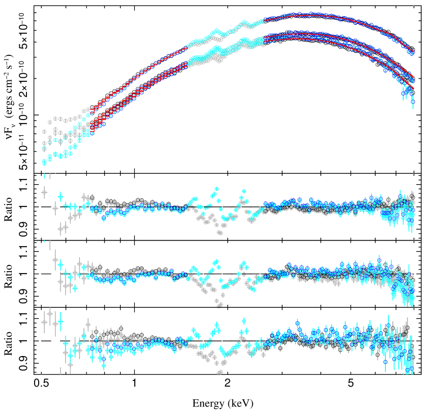
Figure 7.— The joint fit of a simpl$\otimes$kerrbb model to the three spectra assuming a black hole mass and distance of $16\,M_{\odot}$ and 22 kpc. The spectra share a common interstellar absorption column, black hole mass and spin, disk inclination, and a fixed color correction factor of $f_{\rm c}=1.7$. They have independent disk accretion rates and simpl parameters. Black/grey spectra are the combined XIS 0 and 3 spectra, and blue/light blue are the XIS 1 spectra. Lightly shaded data were not included in the fit. The top residuals panel shows the ratio residuals for obsID 405057010, the middle residuals panel shows the ratio residuals for obsID 405057020, and the bottom shows the ratio residuals for obsID 405057030.

As for the Comptonization models, we fit all three observations simultaneously, include a broad Gaussian line in exactly the same manner, and tie some of the model parameters together. Specifically, we constrain each observation to be fit with the same neutral column, line energy and width (fixed to 0.3 keV), and black hole spin, but let the disk accretion rate, the simpl model parameters, and the line normalization be free. Results for these kerrbb model fits are presented in Table 3 and Fig. 7. The resulting fits are good, with the $3\,M_{\odot}$, 10 kpc model yielding $\chi^{2}_{\nu}/\nu=2063/1014$ and the $16\,M_{\odot}$, 22 kpc model yielding $\chi^{2}_{\nu}/\nu=1830/1014$. The latter model is very comparable to our best Comptonization fit. Additionally, this latter, more successful, model has line parameters very similar to those from the Comptonization fits. We also find that only $\approx 7-15\%$ of the disk photons are transferred into a hard tail. The fitted neutral column is slightly smaller than for the Comptonization fits, but only by $\lesssim 10\%$.

Just as the Comptonization models could fit all three observations with a constant normalization (equivalent to a constant inner disk radius), so too can the relativistic disk models fit all three observations with a constant spin parameter (also equivalent to a constant inner disk radius). The main variable parameter among the observations here becomes the disk accretion rate. For both sets of mass and distance assumptions, the fitted spin parameter is high: nearly 0.9 for the $3\,M_{\odot}$, 10 kpc case, and nearly maximally spinning in the other. We discuss the scaling relations among the disk parameters in the next section.

4. Scaling Relations

As shown above, spectral fits to the data are somewhat degenerate. We have found a successful set of relativistic disk model fits assuming a mass of $3\,M_{\odot}$ and a distance of 10 kpc, and also when assuming a mass of $16\,M_{\odot}$ and a distance of 22 kpc. The first set of parameters was chosen as being the lowest mass/closest distance black hole that is likely to be consistent with 4U 1957+11 persistently remaining in a soft state. The second set of parameters was chosen to be consistent with our prior RXTE studies (Nowak et al., 2008), which in turn were found via the scaling relations described below.

As the spectra are dominated by the seed photons from a disk for both the disk and Comptonization models, the flux, $F$, scales as:

$$F\propto\frac{R^{2}}{D^{2}}T^{4}_{\mathrm{eff}}\propto\frac{M^{2}}{D^{2}}\left(\frac{T_{\mathrm{col}}}{f_{\mathrm{c}}}\right)^{4}~{}~{},$$ (2)

where $D$ is the distance to the source, $R$ is the inner radius of the disk, $M$ is the black hole mass, $T_{\mathrm{eff}}$ is the disk’s peak effective temperature, $T_{\mathrm{col}}$ is the disk’s peak color temperature, and $f_{\mathrm{c}}$ is the color correction factor. The effective temperature to the fourth power scales as the fractional Eddington luminosity, $L/\mathrm{L_{Edd}}$, multiplied by $M/R^{2}\propto M^{-1}$. Thus, if we make the assumption that the lowest flux RXTE observations described by Nowak et al. (2008) are indeed at a fixed fraction of Eddington luminosity, e.g., 3%, then we will have:

$$\left(\frac{T_{\mathrm{col}}}{f_{\mathrm{c}}}\right)^{4}\propto M^{-1}~{}~{}.$$ (3)

The color temperature is fixed by observation, and $L/\mathrm{L_{Edd}}\propto\dot{M}/M$ (where $\dot{M}$ is the accretion rate) is fixed by assumption, leading to the first two of our scaling relations:

$$M\propto f_{\mathrm{c}}^{4}~{}~{},~{}~{}\dot{M}\propto f_{\mathrm{c}}^{4}~{}~{}.$$ (4)

Just as the color temperature is fixed by observations, so too is the flux. Given that the disk inner radius scales as mass, and using the fact that the color temperature and flux are fixed by observation, we have that $M^{2}/D^{2}f_{\mathrm{c}}^{4}$ is fixed. Using the above scaling relations, we then obtain:

$$D\propto f_{\mathrm{c}}^{2}~{}~{}.$$ (5)

We have previously used these scaling relations to find spectral fits for a black hole mass of 16 $M_{\odot}$ and a distance of $\approx 22$ kpc (Nowak et al., 2008). Specifically, we first explored fits to RXTE spectra where we fixed the mass and distance to 3 $M_{\odot}$ and 10 kpc. We found that the best fits clustered around a spectral hardening factor of $f_{\mathrm{c}}\approx 1.1$. We then fixed the spectral hardening factor to $f_{\mathrm{c}}=1.7$ and the mass to 16 $M_{\odot}$. We allowed the distance to be a free parameter, and found that its best fit values clustered around 22 kpc, i.e., roughly consistent with the scaling relations above.

Here we perform a similar exercise for the Suzaku spectra. As in Section 3, we fit all three spectra simultaneously with the simpl$\otimes$kerrbb model wherein we only allow the accretion rate and simpl parameters to vary among the three spectra. We consider two sets of fits, one with mass of 3 $M_{\odot}$ and distance 10 kpc, and another with 16 $M_{\odot}$ and distance 22 kpc. For both we allow the black hole spin to be a free parameter, and we create grids of fits for fixed spectral hardening factors ranging over $f_{\mathrm{c}}=1.1$–3.7. The plot of fitted spin, $a^{*}$, vs. spectral hardening factor, $f_{\mathrm{c}}$, is presented in Fig. 8.

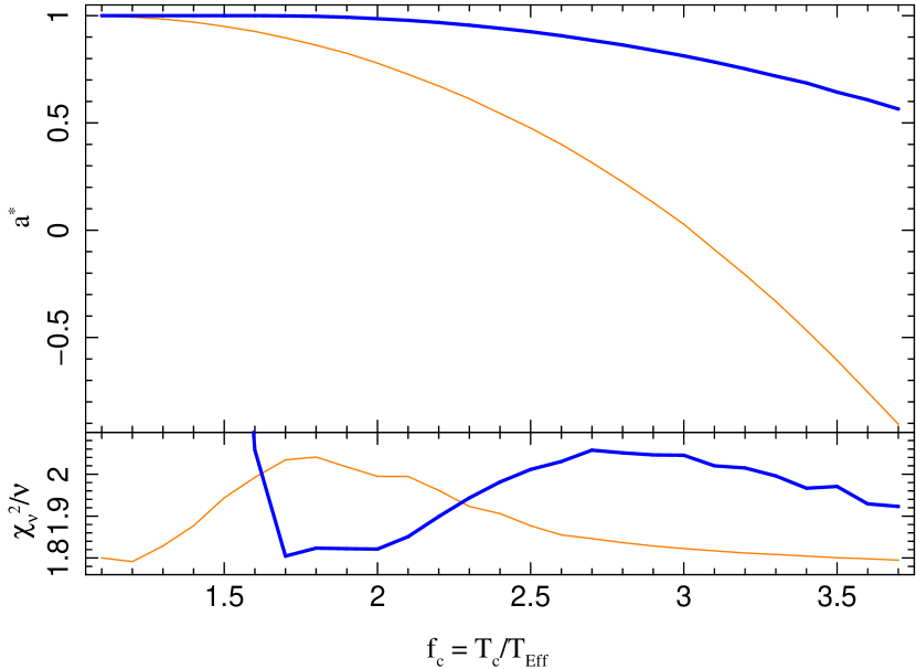
Figure 8.— Results of fitting a simpl$\otimes$kerrbb to the three Suzaku observations of 4U 1957+11. The top panel shows the fitted spin vs. spectral hardening factor. The bottom panel shows the reduced $\chi^{2}$ value of the fits. The blue (thicker) lines represent models with the mass and distance fixed to 16 $M_{\odot}$ and 22 kpc, respectively, and orange lines represent models with the mass and distance fixed to 3 $M_{\odot}$ and 10 kpc, respectively.

As for our prior RXTE observations, we find that fits using $3\,M_{\odot}$, 10 kpc, and $f_{\mathrm{c}}=1.1$ or $16\,M_{\odot}$, 22 kpc, and $f_{\mathrm{c}}=1.7$ are nearly equally good and are of comparable $\chi^{2}$ to our best Comptonization fits. We also see that all fits using $16\,M_{\odot}$, and 22 kpc require large spin parameters. The fits using $3\,M_{\odot}$ and 10 kpc only achieve low spin parameters for large color correction factors, $f_{\mathrm{c}}\gtrsim 3$. (These conclusions are unaltered if uniform 1.35% systematic errors are included in the fits.)

5. Discussion

There are four salient features of these Suzaku observations of 4U 1957+11 that echo the results that we obtained with our prior Chandra, XMM-Newton, and RXTE studies. The peak disk temperatures are high, the disk normalizations (or equivalently, emitting areas or inner disk radii) are small, all observations can be fit with the same inner disk radius, and the spectra are remarkably simple. The only significant deviations from a simple continuum, aside from spectral hardening and a possible weak, broad Fe line at high energy, are $\approx 0.7$–$0.9$ keV features associated with absorption by the ISM, predominantly due to the Fe L and Ne edges.

We show a closeup of this region in Fig. 9. The spectral feature seen at $\approx 0.55$ keV, not described by our fitted models, can in fact be seen in the flux corrected spectra of any monochromatic, narrow line spectrum simulated using the Suzaku response functions. Small calibration errors in the amplitude of this feature potentially could lead to a systematic underestimate or overestimate of the predicted counts near 0.55 keV. We thus do not believe that this feature is indicative of physical complexity in the underlying 4U 1957+11 spectra. Likewise, it is unclear whether the $\approx 5\%$ residuals seen near the 0.7 keV Fe L edge represent complexity in the physical spectrum, as opposed to uncertainty in the response. Aside from the Fe L edges, Chandra and XMM-Newton spectra did not show any spectral features near the 0.7 keV bandpass (Nowak et al., 2008).

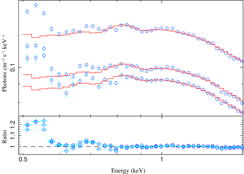
Figure 9.— The same fit as seen in Fig. 5, but showing the XIS 0, 1, and 3 spectra combined, and the model applied down to 0.5 keV.

The only clear spectral features are the Ne edge/Ne ix absorption near 0.9 keV. Similarly simple disk spectra were implied by Suzaku observations of LMC X-3 in its soft, disk dominated state (Kubota et al., 2010). As pointed out by Kubota et al. (2010), such spectral simplicity is in fact surprising if modern disk atmosphere models apply to these sources. These disk atmosphere models predict spectral structure with $\pm 5\%$ amplitude near metal edges (Davis & Hubeny, 2006) that is seen neither here nor in Suzaku observations of LMC X-3. That the simplest, phenomenological disk models lacking such features describe the spectra extremely well (i.e., to within $\lesssim 5$% 0.7–0.8 keV, and to $\lesssim 2\%$ above 0.8 keV) is quite remarkable, and may indicate that additional physics needs to be incorporated into the disk atmosphere models (Kubota et al., 2010).

We also have confirmed the results of our prior studies in that the best fits assuming a small mass and distance (3 $M_{\odot}$, 10 kpc) require a black hole spin $a^{*}\gtrsim 0.9$. The required spin increases if we instead assume 16 $M_{\odot}$ and 22 kpc. Altering the assumed disk inclination does not change this situation. Higher disk inclinations are ruled out by the lack of system eclipses. Lower disk inclinations allow for more observed gravitational redshifting, and less relativistic beaming, of the spectrum, and thus require larger spectral correction factors. (I.e., inclination effects more than just the projected area of the disk.) As an example, we took the 16 $M_{\odot}$ and 22 kpc kerrbb model, froze the inclination to $45^{\circ}$ and let both the black hole spin and hardness correction factor become free parameters. A solution with $\chi^{2}$ comparable to the best fits discussed above was found, however, it required maximally negative spin of $a^{*}\approx-1$ and an extremely large color correction factor of $\approx 8$. Thus, high spin/high inclination solutions are the most “straightforward” solutions that we have been able to obtain, and generally have had the lowest color-correction factors of the models that we have explored (see also Nowak et al., 2008).

These results are in fact confirmed by the Comptonization model fits: the high disk temperatures (1.31–1.48 keV) and especially the low normalization — 15 times lower than expected for a $3\,M_{\odot}$ Schwarzschild black hole at 10 kpc — could be indicative of a rapidly spinning black hole. As discussed above, the disk temperature in the diskpn seed photons used in the Comptonization model peaks at $\approx 10\,GM/c^{2}$. If one were to reduce this radius to $\approx 2.5\,GM/c^{2}$, i.e., change the emission profile to more closely match that of a rapidly spinning hole, then the Comptonization model normalization would be consistent with a $3\,M_{\odot}$ black hole at only 10 kpc.

The Comptonization models offer two possibilities for fitting the 4U 1957+11 spectrum with a low spin. The first, perhaps less likely, possibility is to increase the color-correction factor via a low temperature, optically thick corona. We have already seen that the lowest flux observations are fit with such coronae, albeit with a Compton $y$-parameter of $\approx 0.1$. Instead, we are envisioning a scenario wherein $y\approx f_{\mathrm{c}}\approx 3$ – the color correction value required to fit a $3\,M_{\odot}$, 10 kpc, Schwarzschild black hole. This would require an optical depth of

$$\tau\approx 9.8\left(\frac{4\,\mathrm{keV}}{kT_{\mathrm{c}}}\right)^{1/2}\left(\frac{f_{\mathrm{c}}}{3}\right)^{1/2}~{}~{},$$ (6)

where $kT_{\mathrm{c}}$ is the coronal temperature. This is a coronal regime typically not explored in spectral models. The concept would be that the low flux, equilibrium solution of the disk was such a cool, optically thick atmosphere which at higher flux (i.e., the 15% of the time requiring a hard tail) expanded into a hot, optically thin corona.

Aside from lacking a theoretical description of such a scenario, the fitted constant emitting area at low flux implies that the 4U 1957+11 system must always return to the same equilibrium coronal solution at low flux. It is not clear why this should be the case. The second possibility offered by the Comptonization solutions is simply to increase the distance to 4U 1957+11, while keeping the mass small. The scaling relations discussed in Section 4 only apply under the assumption that the lowest flux observations are a fixed fraction of the Eddington luminosity (e.g., 2% $\mathrm{L_{Edd}}$). If we relax this assumption, then eq. 1 suggests that if the 4U 1957+11 distance were 40 kpc, then it could be a $3\,M_{\odot}$ Schwarzschild black hole. This would imply, however, that the faintest 4U 1957+11 spectra are $\gtrsim 30\%\,\mathrm{L_{Edd}}$, while the brightest observed RXTE spectra are $\gtrsim\mathrm{L_{Edd}}$. This would be rather unusual, especially given the lack of strong variability found in the RXTE spectra: the root mean square variability is typically $\lesssim 3\%$, and at its strongest was $\lesssim 13\%$ in the 2–60 keV bandpass over $\approx 10^{-2}$–$2\times 10^{3}$ Hz (Nowak & Wilms, 1999; Nowak et al., 2008).

It therefore seems likely that 4U 1957+11 is a system that has a combination of both high spin and large distance, which puts this X-ray binary in the Galaxy’s halo. It is interesting to speculate whether these two characteristics are related to one another. First, we note the obvious fact that in order for 4U 1957+11 to be a X-ray binary it must still be accreting and therefore be a comparatively young system. Given the low star formation rate in the Galaxy’s halo, it is rather unlikely, therefore, that 4U 1957+11 was formed in the halo. Instead 4U 1957+11 likely originates in the Galactic disk and then migrated into the halo. Several possible formation scenarios have been discussed in the literature, most recently associated with the discovery of young hypervelocity stars in the Galaxy’s halo. For example, Perets (2009, and references therein) discuss a scenario where hypervelocity binary systems are created through the interaction of a hierarchical triple star system with the supermassive black hole in the center of the Galaxy. Since hierarchical triples are very common among multiple star systems, such a scenario is likely. With a typical ejection velocity of 1800 $\mathrm{km}\,\mathrm{s}^{-1}$, it would take this system a few $10^{6}$ years to reach its current position, well within the lifetime of typical evolution scenarios for X-ray binary systems (van den Heuvel, 1976). (At such a velocity, and assuming a 22 kpc distance, the proper motion of 4U 1957+11 likely would have amounted to $\mathrel{\hbox to0.0pt{\raise 2.20013pt\hbox{$<$}\hss}{\lower 2.20013pt\hbox{$\sim$}}}0.3^{\prime\prime}$ since the discovery of the optical counterpart by Margon et al. 1978.) Such a scenario could also explain a large spin for the system, if during the ejection angular momentum is transferred onto the black hole.

A high black hole spin for 4U 1957+11 is a consistent interpretation of the results presented here; however, such a result is dependent upon the unknown mass, distance, and inclination of the system. Given the nature of 4U 1957+11 as perhaps the simplest, cleanest example of a BHC soft state, and perhaps the most rapidly spinning black hole, observations to independently determine this system’s parameters are urgently needed.

References

- Bayless et al. (2011) Bayless, A., Robinson, E., Mason, P., & Robertson, P. 2011, ApJ, 730, 43
- Coppi (1999) Coppi, P., 1999, PASP Conference Series, 161, 375
- Davis et al. (2005) Davis, S. W., Blaes, O. M., Hubeny, I., & Turner, N. J. 2005, ApJ, 621, 372
- Davis et al. (2006) Davis, S. W., Done, C., & Blaes, O. M. 2006, ApJ, 647, 525
- Davis & Hubeny (2006) Davis, S. W., & Hubeny, I. 2006, ApJS, 164, 530
- Dunn et al. (2010) Dunn, R. J. H., Fender, R. P., Körding, E. G., et al. 2010, MNRAS, 403, 61
- Gierliński et al. (1999) Gierliński, M., Zdziarski, A. A., Poutanen, J., et al. 1999, MNRAS, 309, 496
- Hakala et al. (1999) Hakala, P. J., Muhli, P., & Dubus, G. 1999, MNRAS, 306, 701
- Houck & Denicola (2000) Houck, J. C., & Denicola, L. A. 2000, in ASP Conf. Ser. 216: Astronomical Data Analysis Software and Systems IX, Vol. 9, 591
- Koyama et al. (2007) Koyama, K., Tsunemi, H., Dotani, T., et al. 2007, PASJ, 59, 23
- Kubota et al. (2010) Kubota, A., Done, C., Davis, S. W., et al. 2010, ApJ, 714, 860
- Li et al. (2005) Li, L.-X., Zimmerman, E. R., Narayan, R., & McClintock, J. E. 2005, ApJS, 157, 335
- Maccarone (2003) Maccarone, T. J., 2003, A&A, 409, 697
- Margon et al. (1978) Margon, B., Thornstensen, J. R., & Bowyer, S. 1978, ApJ, 221, 907
- Mitsuda et al. (2007) Mitsuda, K., Bautz, M., Inoue, H., et al. 2007, PASJ, 59, 1
- Mitsuda et al. (1984) Mitsuda, K., Inoue, H., Koyama, K., et al. 1984, PASJ, 36, 741
- Nowak et al. (2011) Nowak, M. A., Hanke, M., Trowbridge, S. N., et al. 2011, ApJ, 728
- Nowak et al. (2008) Nowak, M. A., Juett, A., Homan, J., et al. 2008, ApJ, 689, 1199
- Nowak & Wilms (1999) Nowak, M. A., & Wilms, J. 1999, ApJ, 522, 476
- Nowak et al. (2001) Nowak, M. A., Wilms, J., Heindl, W. A., et al. 2001, MNRAS, 320, 316
- Perets (2009) Perets, H. B., 2009, ApJ, 698, 1330
- Russell et al. (2010) Russell, D., Lewis, F., Roche, P., Clark, J.S. Breedt, E., & Fender, R. 2010, MNRAS, 402, 2671
- Russell et al. (2011) Russell, D. M., Miller-Jones, J. C. A., Maccarone, T. J., et al. 2011, ApJ, 739, L19
- Shafee et al. (2006) Shafee, R., McClintock, J. E., Narayan, R., et al. 2006, ApJ, 636, L113
- Shakura & Sunyaev (1973) Shakura, N. I., & Sunyaev, R. 1973, A&A, 24, 337
- Steiner et al. (2009) Steiner, J. F., Narayan, R., McClintock, J. E., & Ebisawa, K. 2009, PASP, 121, 1279
- Takahashi et al. (2007) Takahashi, T., Abe, K., Endo, M., et al. 2007, PASJ, 59, 35
- Thorstensen (1987) Thorstensen, J. R., 1987, ApJ, 312, 739
- Uchiyama et al. (2008) Uchiyama, Y., Maeda, Y., Ebara, M., et al. 2008, PASJ, 60, 35
- van den Heuvel (1976) van den Heuvel, E. P. J., 1976, in Structure and Evolution of Close Binary Systems, ed. P. Eggleton, S. Mitton, & J. Whelan, Vol. 73, IAU Symposium, 35
- Wijnands et al. (2002) Wijnands, R., Miller, J., & van der Klis, M. 2002, MNRAS, 331, 60
- Wilms et al. (2000) Wilms, J., Allen, A., & McCray, R. 2000, ApJ, 542, 914
- Wilms et al. (2001) Wilms, J., Nowak, M. A., Pottschmidt, K., et al. 2001, MNRAS, 320, 316
- Yao et al. (2008) Yao, Y., Nowak, M. A., Wang, Q. D., Schulz, N. S., & Canizares, C. R. 2008, ApJ, 672, L21