Reducing sequencing complexity in dynamical quantum error suppression
by Walsh modulation

Abstract

We study dynamical error suppression from the perspective of reducing sequencing complexity, in order to facilitate efficient semi-autonomous quantum-coherent systems. With this aim, we focus on digital sequences where all interpulse time periods are integer multiples of a minimum clock period and compatibility with simple digital classical control circuitry is intrinsic, using so-called Walsh functions as a general mathematical framework. The Walsh functions are an orthonormal set of basis functions which may be associated directly with the control propagator for a digital modulation scheme, and dynamical decoupling (DD) sequences can be derived from the locations of digital transitions therein. We characterize the suite of the resulting Walsh dynamical decoupling (WDD) sequences, and identify the number of periodic square-wave (Rademacher) functions required to generate a Walsh function as the key determinant of the error-suppressing features of the relevant WDD sequence. WDD forms a unifying theoretical framework as it includes a large variety of well-known and novel DD sequences, providing significant flexibility and performance benefits relative to basic quasi-periodic design. We also show how Walsh modulation may be employed for the protection of certain nontrivial logic gates, providing an implementation of a dynamically corrected gate. Based on these insights we identify Walsh modulation as a digital-efficient approach for physical-layer error suppression.

I Introduction

Dynamical quantum error correction has been proposed as a strategy by which arbitrarily accurate evolutions may in principle be implemented in a large class of open quantum systems. This approach involves application of open-loop control protocols at the physical level Viola and Lloyd (1998); Viola et al. (1999); Zanardi (1999); Vitali and Tombesi (1999); Viola and Knill (2003); Byrd and Lidar (2003); Kofman and Kurizki (2004); Khodjasteh and Lidar (2005); Yao et al. (2007); Uhrig (2007); Gordon et al. (2008); Khodjasteh and Viola (2009a, b); Khodjasteh et al. (2010); Yang et al. (2010); Biercuk et al. (2011); through time-dependent modulation of the system’s dynamics, the effects of an environment which fluctuates sufficiently slowly are coherently averaged out. Dynamical decoupling (DD) is an experimentally validated Ladd et al. (2005); Fraval et al. (2005); Krojanski and Suter (2006); Biercuk et al. (2009a, b); Du et al. (2009); West et al. (2009); Damodarakurup et al. (2009); Szwer et al. (2011); Álvarez et al. (2010); de Lange et al. (2010); Sagi et al. (2010); Bluhm et al. (2011); Barthel et al. (2010); Ryan et al. (2010); Bylander et al. (2011); Medford et al. (2011) subclass of these protocols specifically tailored to the task of suppressing decoherence during the implementation of the identity operator – resulting in improved quantum storage.

DD takes physical inspiration from the spin echo in nuclear magnetic resonance (NMR) Hahn (1950); Haeberlen (1976); Vandersypen and Chuang (2004), and relies on deterministic (periodic Viola and Lloyd (1998) or aperiodic Khodjasteh and Lidar (2005); Uhrig (2007)), or even random Viola and Knill (2005); Santos and Viola (2006) modulation of the idle system via pulsed control. A proliferation of analytical formalisms and new DD schemes has appeared in the literature, in particular for the paradigmatic case of a single qubit exposed to pure (classical and/or quantum) dephasing Viola and Lloyd (1998); Faoro and Viola (2004); Uhrig (2007, 2008); Kuopanporttii et al. (2008); West et al. (2009); Biercuk et al. (2009a); Uys et al. (2009); Hodgson et al. (2010); Khodjasteh et al. (2011). While an understanding of the performance of these sequences may be unified by the application of a noise filtering framework Martinis et al. (2003); Kofman and Kurizki (2004); Cywinski et al. (2008); Ajoy et al. (2011); Biercuk et al. (2011), each sequence brings particular requirements for the necessary pulse timings, often incorporating nonintuitive analytical expressions or numerical search to define pulse locations in a sequence. As a result, the generation of DD pulse sequences at the lab bench is usually accomplished using specially programmed microcontrollers or a PC under user control.

In this work, we address the problem of control complexity in dynamical error correction, introducing a set of digital DD protocols optimized for hardware compatibility and minimization of sequencing complexity. These protocols are based on the Walsh functions Beauchamp (1975); Tzafestas (1985), which take binary values and are composed of products of square waves, forming an orthonormal basis similar to the sines and cosines. The Walsh functions benefit from compact notation and a uniform mathematical basis for sequence construction. We describe the error-suppressing properties of Walsh modulation and Walsh dynamical decoupling (WDD), and introduce a quantitative metric for sequencing complexity, $r$, the number of Rademacher square-wave functions which must be multiplied (or added mod-2) in hardware to generate the control propagator for that sequence. The Rademacher functions in turn can be trivially generated via elementary digital circuits synchronous with a distributed clock signal. Thus, by construction Walsh modulation is highly compatible with simple digital sequencing circuitry and digital clocking as may be needed in large or semi-autonomous systems. This approach therefore provides efficient error suppression, important for real-world implementations beyond simple demonstration experiments.

The remainder of this manuscript is organized as follows. After introducing the relevant system and control setting in Section II, Section III is devoted to describing the mathematical formulation and key features of the Walsh functions, and their natural use in defining WDD schemes. In this section, our main results are established, including an exact relationship between the sequencing complexity $r$ and the order of decoherence suppression in the perturbative limit. Here, we also describe the entire taxonomy of WDD sequences, discussing relationships between WDD and well-known sequences, as well as characterizing new DD sequences with digital timing. In Sec. IV, we discuss extensions of the WDD formalism beyond the simplest setting of a single qubit exposed to classical dephasing noise. In particular, we show how two-axis generalizations of WDD naturally recover and expand existing concatenated DD schemes, and discuss how Walsh modulation allows enhancement of the fidelity of nontrivial gate operations, examining a recent trapped-ion experiment as an example Hayes et al. (2011). We follow this with an analysis of the explicit benefits of WDD over other optimized DD approaches in Sec. V, and close with a brief summary and outlook. A proof of WDD error suppression properties from Rademacher functions is included in Appendix A for completeness.

II Physical Setting

DD is applicable to a variety of non-Markovian error models (including arbitrary many-qubit systems interacting with quantum environments, Viola et al. (1999); Wang and Liu (2011)) and can address non-ideal pulses or continuous control scenarios (as in Eulerian DD Viola and Knill (2003)). Our starting point here, however, is the simplest yet practically important case of a single qubit subject to classical phase noise and controlled with ideal $\pi$ pulses. In this setting, the qubit is affected by an undesired noise Hamiltonian,

$$H_{\text{noise}}=\beta(t)\sigma_{z},$$ (1)

where $\beta(t)$ is a stochastic process and $\sigma_{i}$ denote the Pauli matrices for $i=x,y,z$. We assume that the system can be controlled by application of idealized sequences of qubit rotations, each corresponding to a $\pi$ rotation around the $x$ axis, i.e., to the unitary operator $\sigma_{x}$. Each sequence is characterized by the pulse timings $\{t_{j}\}_{j=1}^{s}$, where $t_{0}=0$ and $t_{s+1}=\tau$ denote the initial (preparation) and final (readout) times respectively. We use $\delta_{j}=t_{j}/\tau$ to denote the “normalized pulse locations” and the “pulse pattern” $p=\{\delta_{j}\}_{j=1}^{s}$, to distinguish among various sequences with the same running time not (a).

During the evolution, the $\pi$ pulses implement the control propagator

$$U_{c}(t) = \sigma_{x}^{[y(t)+1]/2},$$

where $y(t)$ takes values $\pm 1$ and switches instantaneously between these values at times corresponding to application of the $\pi$ pulses. For brevity, we shall refer to $y(t)$ as the “sequence propagator” in what follows. The “filter function” $F_{p}(\omega\tau)$ associated with the pulse pattern $p=\{\delta_{j}\}$ and sequence duration $\tau$ is defined in terms of $\tilde{y}(\omega\tau)$, the Fourier transform of the sequence propagator Cywinski et al. (2008); Uhrig (2008):

$$F_{p}(\omega\tau) =\omega^{2}|\tilde{y}(\omega\tau)|^{2}$$ (2)

$$=\Big{|}\sum\limits_{j=0}^{s}(-1)^{j}(e^{i\delta_{j}\omega\tau}-e^{i\delta_{j+1}\omega\tau})\Big{|}^{2}.$$ (3)

The case of free evolution (also referred to as free induction decay, FID, in NMR terminology) is formally included by letting $s=0$.

The presence of the noise Hamiltonian (1) implies a coherence loss at the readout due to phase randomization, resulting from the ensemble average with respect to noise realizations. The action of DD is to break the system’s evolution into a sequence of interactions with the environment with alternating signs, resulting in significantly reduced phase accumulation at the end of the sequence Viola and Lloyd (1998); Viola et al. (1999). This may be effectively represented as the expected value of the convolution of the stochastic noise term with the sequence propagator Haeberlen (1976); Uhrig (2007, 2008); Cywinski et al. (2008); Biercuk et al. (2011). In particular, the filter function provides a compact exact expression for the coherence decay under Gaussian noise; if the system is prepared in a superposition of eigenstates of $\sigma_{z}$, its coherence $W\equiv|\overline{\langle\sigma_{+}\rangle(\tau)}|$ decays as $e^{-\chi_{p}(\tau)}$, where

$$\chi_{p}(\tau)=\frac{2}{\pi}\int\limits_{0}^{\infty}\frac{S_{\beta}(\omega)}{\omega^{2}}F_{p}(\omega\tau)d\omega,$$ (4)

and $S_{\beta}(\omega)$ is the power spectrum of the noise $\beta(t)$. While nominally the integration range in Eq. (4) is infinite, in practice $S_{\beta}(\omega)$, and thus the “spectral measure” $\lambda(\omega)\equiv S_{\beta}(\omega)/2\pi\omega^{2}$ Khodjasteh et al. (2011), is significant only for frequencies smaller than an ultraviolet cut-off frequency $\omega_{c}$. The filter function can also be employed for a qubit coupled to a purely-dephasing quantum bosonic environment with a similar expression for decoherence under DD sequences Viola and Lloyd (1998); Uhrig (2007). The effect of continuous control can also be approximated within the filter function formalism as long as terms that are of second order and higher in $H_{\text{noise}}$ are ignored Kofman and Kurizki (2004); Gordon et al. (2008) (see also Sec. IV).

The filter function enters the integrand in Eq. (4) as a multiplicative factor of $\lambda(\omega)$, therefore, as long as $F_{p}(\omega\tau)$ is small for $\omega<\omega_{c}$, the coherence loss will also remain small, as desired. Determining the actual value of $\chi_{p}(\tau)$ requires a detailed knowledge of $S_{\beta}(\omega)$, yet we may compare the coherence associated with various DD sequences (including free evolution) by directly comparing their corresponding filter functions over the interval $[0,\omega_{c}\tau$]. For all sequences the filter function vanishes at zero, however we may differentiate the low-frequency behaviors (rates of growth) among various timing patterns. Let the low-frequency behavior of the filter function be given by

$$F_{p}(\omega\tau)\propto(\omega\tau)^{2(\alpha+1)},$$ (5)

corresponding to

$$\tilde{y}(\omega\tau)\propto(\omega\tau)^{\alpha}.$$

In the language of filter design Biercuk et al. (2011), Eq. (5), defines a “highpass filter” with a “rolloff” of $6(\alpha+1)\text{dB}/\text{octave}$. As long as the cutoff frequency $\omega_{c}$ is sufficiently small, the low-frequency behavior of the filter function translates to

$$1-W\propto(\omega_{c}\tau)^{2\alpha+1}.$$

For example, the filter function for free evolution $F_{\{0,1\}}(\omega\tau)=2\sin^{2}(\omega\tau/2)$ corresponds to $\alpha=0$, while high-order DD sequences have larger positive $\alpha$’s. The frequency range over which the filter function suppresses noise is given by the “bandwidth” $\Omega_{p}$, roughly defined as the largest frequency below which $F_{p}(\omega\tau)\leq 1$, a value approximately commensurate with the value $\omega_{F1}$ introduced in previous analyses of the filter function Biercuk et al. (2011). Large values of the bandwidth $\Omega_{p}$ improve the high-frequency robustness of a particular DD sequence and allow it to be used with comparatively lower pulse rates.

III Dynamical Decoupling by Digital Modulation

Many previously developed schemes for DD rely on access to sequences defined in continuous time, which is a good approximation for most benchtop experiments conducted today. In the long term, however, where large systems with error rates deep below the fault-tolerance threshold are required, these approximations will cease to provide an accurate estimate of residual error rates. Previous work has shown that the benefits of optimized sequences such as UDD become diminished in such cases where we expect the use of digital control and discretized time Biercuk et al. (2011). We are thus motivated to find digital modulation schemes that are both intrinsically compatible with discrete time and with the digital control hardware that will inevitably be employed in sequencing.

We define two relevant timescales for such a modulation scheme; the total running time $\tau$, and a minimum interval (minimum switching time Khodjasteh et al. (2011)) given by

$$\tau_{\text{min}}=\tau/2^{m},$$

where $2^{m}$ is the largest possible number of free-evolution periods in an applied sequence. In practice, $\tau_{\text{min}}$ is bounded from below by technological constraints such as modulation rates or hardware clock speeds. In the case of digital modulation, all interpulse periods must be defined as integer multiples of $\tau_{\text{min}}$. This in turn places constraints on the allowed values of ${\delta_{j}}$ in a sequence. Irrational values of fractional pulse locations have intrinsic conflict with digital modulation, thus mandating alternate approaches.

In order to overcome this challenge, we have identified the Walsh functions as a mathematical basis that is compatible with digital sequencing hardware. In this section we discuss the Walsh functions and the WDD derived from them.

III.1 Walsh functions and WDD

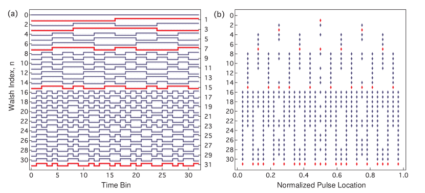
Figure 1: (color online) Walsh functions listed by Paley ordering. (a) The first 32 Walsh functions. (b) The normalized pulse locations, $\delta_{j}$, corresponding to the digital transition points of Walsh functions. Sequences $\text{WDD}_{2^{r}-1}$ are highlighted in both panels.

The Walsh functions are a family of binary valued ($\pm 1$) piecewise-constant functions on the $[0,1]$ interval Walsh (1923). They found a place in engineering in the 1960s, when they started being applied to problems ranging from communications and signal analysis to image processing, and noise filtering Beauchamp (1975); Tzafestas (1985). The Walsh functions come in a variety of labeling conventions, including the Hadamard, “sequency”, and Paley (or dyadic). In particular, the sequency ordering counts the number of “switchings” of the Walsh functions. In this paper, however, we focus on the Paley ordering, given in terms of the so-called Rademacher functions Rademacher (1922), which are defined as

$$\textsf{R}_{j}(x)=\textrm{sgn}\left[\sin\left(2^{j}\pi x\right)\right],\;\;j\geq 0,$$

and correspond to periodic digital switchings between $\pm 1$ over $[0,1]$ with the “rate” $2^{j}$. The Walsh function of Paley order $n$, $\textsf{W}_{n}(x)$, is then defined as Paley (1932)

$$\textsf{W}_{n}(x) = \prod_{j=1}^{m}\textsf{R}_{j}(x)^{b_{j}},\;\;\;x\in[0,1],$$ (6)

where we denote by $(b_{m}b_{m-1}...b_{1})_{2}$ the binary representation of $n$, that is, $n=b_{m}2^{m-1}+b_{m-1}2^{m-2}+\ldots+b_{1}2^{0}$. The actual number, $r$, of Rademacher functions used in constructing a Walsh function, is the Hamming weight (number of non-zero binary digits) of $n$. For illustration, the Walsh functions $\{\textsf{W}_{n}(x)\}_{n=1}^{32}$ in the Paley ordering are shown in Fig. 1(a). The Walsh functions form an orthonormal basis over $[0,1]$, that is,

$$\int_{0}^{1}\textsf{W}_{n}(x)\textsf{W}_{m}(x)dx=\delta_{mn},$$ (7)

where $\delta_{mn}$ is the Kronecker delta. Any integrable function $f(x)$ defined over $[0,1]$ has a convergent Walsh-Fourier expansion similar to the usual Fourier series:

$$f(x)=\sum_{n=0}^{\infty}a_{n}\textsf{W}_{n}(x),\;\;a_{n}=\int_{0}^{1}f(x)\textsf{W}_{n}(x)dx.$$ (8)

This allows us to expand any sequence propagator in the Walsh basis. We note in passing that the Walsh basis is technically over-complete while the Rademacher functions form an orthonormal system Rademacher (1922).

We define the Walsh DD (WDD) sequences directly based on the Walsh functions: that is, for a given running time $\tau$, the sequence $\text{WDD}_{n}$ is determined by the control propagator

$$y(t)=\textsf{W}_{n}(t/\tau),\;\;t\in[0,\tau].$$ (9)

Equivalently, we may specify the normalized pulse locations for $\text{WDD}_{n}$ as the switching locations of $\textsf{W}_{n}(x)$, whereas the constant pieces of the Walsh functions correspond to interpulse delays. By construction, the number of pulses used in $\text{WDD}_{n}$ is given by the sequency $s$ associated with $\textsf{W}_{n}$. More explicitly, if in binary notation $n=(b_{m}b_{m-1}...b_{1})_{2}$ and $s=(g_{m}g_{m-1}...g_{1})_{2}$, then $g_{i}=b_{i}+b_{i+1}\text{mod 2}$ not (b), known as a Gray code.

Both the total running time, $\tau$, and the minimum switching time, $\tau_{\text{min}}=\tau/2^{m}$, impose constraints on the accessible WDD sequences. First, we must have $m=O(\log_{2}n)$, the number of digits in the binary representation of $n$ for a given WDD sequence. Once these parameters are fixed, there is a maximum value $n\approx O(\tau/\tau_{\text{min}})$ for which $\text{WDD}_{n}$ is viable. Reversing this argument, by focusing on a finite set of $\text{WDD}_{n}$ and a fixed running time, we automatically accommodate a finite minimum switching time.

Figure 1(b) depicts the pulse locations plotted as $\delta_{j}$ for a normalized sequence duration $\tau=1$ extracted from the $\textsf{W}_{32}(t/\tau)$. Some familiar DD sequences are immediately identified: $\text{WDD}_{1}$ is the spin echo sequence and $\textrm{WDD}_{3}$ is the two-pulse Carr-Purcell-Meiboom-Gill (CPMG) pulse sequence. We will return to these correspondences in Section III.3.

III.2 Error suppression properties

A primary aim in the construction of DD sequences is to increase the order of error suppression, resulting in better cancellation of noise at sufficiently low frequencies Uhrig (2007, 2008); Lee et al. (2008); Cywinski et al. (2008); Yang and Liu (2008). In order to characterize the error suppression capabilities of WDD sequences, we begin by noting that the Walsh functions, constructed as products of $r$ Rademacher functions [Eq. (6)] satisfy the following important equality (see Appendix for an explicit proof):

$$\int_{0}^{1}[\textsf{R}_{j_{1}}(x)\cdots\textsf{R}_{j_{r}}(x)]x^{k}dx\equiv 0,\;\;\;k=0,\dots,r-1,$$ (10)

where the $\{j_{k}\}$ indices label the locations of the $r$ non-zero digits in the binary representation of $n$. Equivalently, the monomials $x^{k}$ have no Walsh-Fourier component $a_{n}$ as long as $n$ has a Hamming weigth of at least $k$. Let us focus on the Fourier transform of the propagator function for $\text{WDD}_{n}$. Using Eqs. (2) and (9) we have:

$$\tilde{y}(\omega\tau)= \>\tau\int_{0}^{1}\textsf{W}_{n}(x)e^{i\omega\tau x}dx,$$

$$= \>\tau\int_{0}^{1}\textsf{R}_{j_{1}}(x)\cdots\textsf{R}_{j_{r}}(x)\sum_{k=r}^{\infty}\frac{(i\omega\tau x)^{k}}{k!}dx,$$

where the powers of $x$ below $r$ have been eliminated by using Eq. (10). Together with Eq. (2), the above equation implies that

$$F_{\text{WDD}_{n}}(\omega\tau)\propto(\omega\tau)^{2(r+1)}.$$ (11)

Thus, $\text{WDD}_{n}$ suppresses errors up to order $r$. Expressed differently, all $\text{WDD}_{n}$ derived from Walsh functions composed of $r$ Rademacher functions exhibit the same order of error suppression. The relationship between $r$, the Hamming weight of the Walsh order $n$, and the order of error suppression is one of the main results of this work.

The error-suppressing properties of WDD_n can also be directly established upon obtaining a compact expression for the corresponding filter function (in analogy to Uhrig (2008)), which is possible by using Eq. (3) in combination with a change of variable $e^{i\omega\tau/2^{m}}\mapsto z$. For $n=(b_{m}\cdots b_{0})_{1}$, the filter function for $\text{WDD}_{n}$ is given by

$$F_{\text{WDD}_{n}}(\omega\tau) =\Big{|}(1-z)\prod_{j=1}^{m}(1+(-1)^{b_{j}}z^{2^{j-1}})\Big{|}^{2}$$

$$=4^{m+1}\sin^{2}(\omega\tau_{\text{min}}/2)$$

$$\times\!\prod_{\{j|b_{j}=1\}}\!\!\!\!\sin^{2}(2^{j-2}\omega\tau_{\text{min}}) \times\!\prod_{\{j|b_{j}=0\}}\!\!\!\!\cos^{2}(2^{j-2}\omega\tau_{\text{min}}).$$ (12)

where the product chooses $\sin$ or $\cos$ factors based on the $j$-th binary digit $b_{j}$ of $n$. Interestingly, the trigonometric factors appearing in Eq. (12) have complementary implications for the filter function and ultimately for error suppression. The smallest common period among these terms is at $\omega\tau_{\text{min}}=2\pi$. Each sine term is linear in $\omega\tau$ at $\omega=0$ and each factor of $\sin^{2}(2^{j-2}\omega\tau_{\text{min}})$ subsequently contributes a factor proportional to $(\omega\tau)^{2}$ to the filter function. These combine to give $F_{\text{WDD}_{n}}(\omega\tau)\propto(\omega\tau)^{2(r+1)}$, consistent with Eq. (11). Also, all sine terms have zeroes at $\omega\tau_{\text{min}}=k\pi$ for integer $k$, that correspond to zeroes at $\omega=2^{m}k\pi/\tau$. In contrast, they all carry large maxima occurring at $\omega=O(\tau_{\text{min}}^{-1})$. The cosine terms on the other hand have no effect on the filter function around $\omega=0$, but drop to zero at somewhat higher frequencies (at which the sine terms might be significantly large). This suggests that they can reduce the spikes of the sine terms and contribute to increasing the bandwidth $\Omega_{\text{p}}$.

With the insights above, we find that sequences $\text{WDD}_{2^{r}-1}$ have the lowest value of sequency (pulse number) for a given order of error suppression (among the Walsh family). This is because the binary representation of a digital integer $n=2^{r}-1$ requires all $b_{i}=1$. Figure 2 depicts the filter functions (in a log-log scale) associated with $\text{WDD}_{2^{r}-1}$ for $r=1,\cdots,5$ (as identified in Fig. 1), where we illustrate how the low-frequency rolloff is increased by increasing $r$. We compare the filter functions for these sequences to those of Uhrig DD (UDD), known to provide $s$-order error suppression given $s$ pulses Uhrig (2007, 2008).

In Fig. 2(b) we plot the filter functions for all WDD sequences with $n<32$ and $r=4$. We see that all have the same low-frequency rolloff, validating the assertion that the order of error suppression in a WDD sequence is determined by $r$.

The actual coherence error, $1-W$, associated with a given DD sequence can be calculated by using the relevant power spectrum $S_{\beta}(\omega)$ for the noise in Eq. (4). The presence of spikes in the filter function at $\omega=O(\tau_{\text{min}}^{-1})$ (not shown) implies that we can only expect error suppression as long as $\omega_{c}\tau_{\text{min}}<1$. We can guarantee this by shrinking $\tau_{\text{min}}$ through use of more frequent decoupling pulses, as far as the technological limitations on pulse rates permit this (see Ref. Khodjasteh et al. (2011) for a discussion of the lower bounds on error suppression in DD at constrained minimum switching time).

Fig. 2(c) depicts the performance of $\text{WDD}_{2^{r}-1}$ sequences for a specific illustrative case where a $1/\omega^{2}$ noise power spectral density $S(\omega)$ persists up to a Gaussian high-frequency cutoff $\omega_{c}$ (given in units of inverse time interval $1/\tau$). We have scaled the noise to have a value comparable to that derived from the low-frequency behavior of nuclear spin diffusion in singlet-triplet qubits Biercuk and Bluhm (2011). We observe, as expected, that not only does the calculated $1/e$ coherence time increase with $n$, but the slope of the error accumulation at short times also increases with $n$. This is a manifestation of the increasing order of error suppression with $r$ described above, and shows the utility of high-order WDD sequences for quantum computing applications where minimizing the error probability is of utmost importance Nielsen and Chuang (2000).

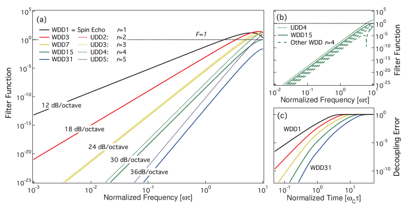
Figure 2: (color online) Error suppression properties of WDD sequences. (a) Filter functions calculated for sequences derived from $W_{2^{r}-1}(t/\tau)$ and corresponding to CDD_r, with fixed total sequence duration, $\tau$. For each value of $r$, the number of fundamental Rademacher functions that are needed to produce the sequence increases, and the order of error-suppression, demonstrated graphically by the low-frequency rolloff of the filter function, increases by 6 dB/octave. Dashed lines correspond to the UDD sequence providing the same order of error suppression. (b) Filter functions for all WDD sequences with $n<32$ and $r=4$. UDD4 is represented by a dashed line and WDD15 by a solid line. Dashed lines correspond, left-to-right, to WDD23, WDD27, WDD29, WDD30. (c) Decoupling error as a function of dimensionless frequency normalized by the cutoff frequency, $\omega_{c}$ in $S_{\beta}(\omega)=\alpha\omega^{-2}\exp{[-(\omega/\omega_{c})^{2}]}$. Here, $\alpha=5\times 10^{16}$, and frequency ranges are set as in Ref. Biercuk and Bluhm (2011). Sequences are same as in (a), and increase in $n$ from left to right.

III.3 The Walsh sequence suite

It is clear from the previous discussion that a number of familiar integer-based DD sequences can be identified as special instances of WDD sequences. These sequences are described next for reference and are summarized in Table 1. For example, periodic DD involves repetitive application of uniformly spaced $\pi$ pulses Viola and Lloyd (1998). A Walsh function composed of a single Rademacher function $R_{k}(x)$ ($r=1$) corresponds to a PDD with $2^{r+1}-1$ pulses. CPMG sequences are modifications of PDD in which the first and last free-evolution periods are half the duration of the interpulse period. We refer to a CPMG sequence with $n$ pulses as $\text{CPMG}_{n}$. A Walsh function of the form $R_{k}(x)R_{k-1}(x)$, with $k\geq 2$, corresponds to $r=2$ and $\text{CPMG}_{2^{k}}$.

We also observe that the sequences defined by $\text{WDD}_{2^{r}-1}$, identified in the previous section, are in fact concatenated DD (CDD) sequences. The latter are known to allow arbitrary orders of error suppression in DD for arbitrary noise models by recursive embedding of a sequence in a “larger” one Khodjasteh and Lidar (2005, 2007). As long as a first-order DD sequence can be implemented in a system, concatenating it with itself results in higher orders of cancellation, at the expenses of increased sequence length. For a purely dephasing environment as examined here, the natural first-order DD sequence (the “base” for concatenation) is the well-known spin-echo sequence, characterized by two equal intervals separated by a $\pi$ pulse; each higher level of concatenation corresponds then to embedding the spin echo in a larger spin echo Cywinski et al. (2008); Hodgson et al. (2010). Using induction, we can show that each concatenation level corresponds to multiplying the sequence propagator by a Rademacher function. This results in a product of all Rademacher functions up to order $r$, thus $b_{1}=\ldots=b_{r}=1$, which corresponds to $\text{WDD}_{2^{r}-1}$. In summary,

$$\text{CDD}_{r}\leftrightarrow\textsf{R}_{1}(x)\cdots\textsf{R}_{r}(x)\leftrightarrow\text{WDD}_{2^{r}-1}.$$ (13)

Again, the WDD sequences that correspond to CDD have a propagator corresponding to a product of Rademachers of all orders from $1$ to $r$, giving $r$-order error suppression with the lowest value of sequency, $s$.

$n$	$\text{WDD}_{n}$	Number of Pulses (Sequency)	Rolloff (dB/octave)
$2^{r}$	PDD	$2^{r+1}-1$	$6\times(1+1)$
$2^{r-1}+2^{r}$	CPMG	$2^{r}$	$6\times(2+1)$
$2^{r}-1$	CDD	$\lceil\frac{2^{r+1}-2}{3}\rceil$	$6\times(r+1)$

Table 1: Familiar sequences among WDD_n. $\lceil x\rceil$ denotes the ceiling function, that is, the smallest integer not less than $x$. The exact expression for the number of pulses in CDD was obtained with the aid of oei .

The WDD family significantly enlarges the sampling set of DD sequences relative to the much more constrained CDD. If the minimum switching time is constrained to $\tau_{\text{min}}=\tau/2^{m}$, then all the $2^{m}$ $\text{WDD}_{n}$ sequences with $n=0,\cdots,2^{m}-1$ are viable. In contrast, the subset of viable CDD sequences for the same fixed total time contains only $m$ sequences, an exponentially smaller number. (However, it remains an even smaller subset of all possible digital DD sequences, which contains $2^{2^{m}}$ sequences. This potential advantage will be discussed in Sec. V.)

WDD thus forms a unifying mathematical framework for the generation of digital DD sequences, including many familiar sequences and a large variety of novel sequences. Using insights derived above, we may fully characterize the structure of arbitrary Walsh functions, and therefore arbitrary WDD modulations. By the structure of the Walsh functions themselves, all WDD sequences can be produced recursively from free evolution by combining the following two intuitive operations:

$\bullet$ Repetition, where the sequence propagator $y(t)$ is repeated identically to produce a longer sequence:

$$y(t) \mapsto \begin{cases}y(t/2),&t<\tau/2,\\ y((t-\tau)/2),&\tau/2<t<\tau.\end{cases}$$

$\bullet$ Concatenation, where the sequence propagator $y(t)$ is repeated with the sign reversed, still yielding a longer sequence:

$$y(t) \mapsto \begin{cases}y(t/2),&t<\tau/2,\\ -y((t-\tau)/2),&\tau/2<t<\tau.\end{cases}$$

The actual implementation of repetition and concatenation may involve inserting a $\pi$ pulse in the middle of the formed sequence to account for the required sign change at $t=\tau/2$. In general, $\text{WDD}_{2n}$ is constructed by repeating $\text{WDD}_{n}$, whereas $\text{WDD}_{2n+1}$ is constructed by concatenating $\text{WDD}_{n}$. For instance, $\text{WDD}_{30}=(\text{WDD}_{15})(\text{WDD}_{15})$ [repetition] and $\text{WDD}_{31}=(\text{WDD}_{15})\pi(\text{WDD}_{15})$ [concatenation], but note the reversal of the role of the middle pulse in $\text{WDD}_{14}=(\text{WDD}_{7})\pi(\text{WDD}_{7})$ [repetition] or $\text{WDD}_{15}=(\text{WDD}_{7})(\text{WDD}_{7})$ [concatenation].

Each concatenation increases the rolloff slope by one order (by contributing an additional sine factor in $F_{\text{WDD}_{n}}$), whereas each repetition does not improve the rolloff (a cosine factor) and may instead increase the bandwidth of the filter, $\Omega_{p}$. This produces a diversity of design features that can be used to improve coherence times (e.g. the $1/e$ decay time denoted $T_{2}$) in addition to coherence values (or, equivalently, error rates) by choosing the appropriate Walsh basis function.

IV Beyond Classical Phase Noise and Quantum Memory

In this section, we consider different extensions of the idea of Walsh modulation to control settings more general than examined thus far.

IV.1 Quantum phase noise

Decoherence in a quantum system is most generically described by the interactions with a quantum environment. We focus first, as before, on a single qubit (see below for multi-qubit extensions). In the absence of control and an internal system Hamiltonian, evolution under the noise Hamiltonian of Eq. (1) is then replaced by evolution under an open-system dephasing Hamiltonian of the form

$$H=H_{SB}+H_{B},\;\;\;H_{SB}=\sigma_{z}\otimes B_{z},$$

where physically $H_{SB}$ represents the interaction term, and $B_{z}$ and $H_{B}$ are generic operators acting on the environment, respectively. Typically, $H_{SB}$ causes entanglement between the system and the environment, which eventually results in loss of phase coherence and mixed qubit states.

The WDD sequences can be applied to the above general quantum dephasing scenario. Under a sequence of $\pi$ pulses, the evolution is identically generated by a piecewise-constant Hamiltonian $\pm\sigma_{z}\otimes B_{z}+H_{B}$. Here, the filter function formalism is not exactly applicable in general. An important exception, as noted, is provided by the case of a bosonic bath Viola and Lloyd (1998); Uhrig (2007); Hodgson et al. (2010), and results accurate up to the second order in $H_{SB}$ have been established in Uchiyama and Aihara (2002) for an arbitrary quantum dephasing environment under periodic DD (see also Kitajima et al. (2010) for exact results on more general classical noise models). Nonetheless, a description based on an effective Hamiltonian and the Magnus expansion can be used to approximate the evolution of the system provided that $\|B_{z}\|$ (operator norm of $B_{z}$) is sufficiently small. Making note of the concatenated and repetitive structure of WDD and following Ref. Khodjasteh and Lidar (2007), we can show that the norm of the effective Hamiltonian for the evolution under $\text{WDD}_{n}$ is given by:

$$\|H_{\text{WDD}_{n}}\|=O[\|B_{z}\|\tau^{r}\max(\|B_{z}\|,\|H_{B}\|)^{r}],$$ (14)

where the strength of the bare interaction $\|B_{z}\|$ is scaled by a factor proportional to $\tau^{r}$, with $r$ denoting, as before, the Hamming weight of $n$. This implies that the expansion of the propagator for the evolution in $\tau$ starts with the power $\tau^{r+1}$. The fidelity loss can be defined as a distance between the ideal state (original state in DD) and the actual propagated state of the system at the end of the evolution (after tracing out the environmental degrees of freedom) Lidar et al. (2008). In the limit of small actions $\tau H_{\text{WDD}_{n}}$, the fidelity loss scales with $\|\tau H_{\text{WDD}_{n}}\|^{2}$ or, equivalently, the qubit fidelity loss scales at worst with $\tau^{2(r+1)}$. While this result mirrors the error cancellation properties of WDD in the filter function formalism [Eq. (11)], we emphasize that asymptotic relationships such as Eq. (14) must be understood as scaling laws that may hide (possibly large) $r$-dependent prefactors. This fact highlights the importance of Eq. (4) as an exact expression for Gaussian phase noise for which a counterpart does not exist in a general quantum-dephasing setting.

IV.2 Generic decoherence

As already mentioned, DD can be applied to a large class of open quantum systems: a control propagator that regularly traverses the elements of the so-called DD group in principle allows suppression of arbitrary non-Markovian decoherence, including multi-qubit noise in many-qubit systems Viola et al. (1999). When the noise operators are decomposed into algebraically independent components, one may reconstruct the generic decoupling procedure through concatenation as well Khodjasteh and Lidar (2007). While the group-theoretic DD design is applicable only to first-order error suppression, concatenation allows us to combine DD sequences for different noise axes to produce a high order and generic decoupling procedure. This idea is the basis of a variety of recent DD schemes, such as quadratic DD (QDD) West et al. (2010) and its multi-qubit variants Wang and Liu (2011); Jiang and Imambekov (2011).

The WDD sequences can be similarly concatenated along different axes to allow suppression of general noise. For example, consider a generalized classical noise Hamiltonian acting on a qubit:

$$H_{\text{noise}}=\beta_{x}(t)\sigma_{x}+\beta_{y}(t)\sigma_{y}+\beta_{z}(t)\sigma_{z},$$

where $\beta_{i}(t)$ are stochastic processes. Applying a WDD sequence with $\sigma_{x}$ pulses effectively removes the $\beta_{y}(t)\sigma_{y}+\beta_{z}(t)\sigma_{z}$ noise component while it leaves $\beta_{x}(t)\sigma_{x}$ intact. Embedding this sequence itself in a WDD sequence with $\sigma_{y}$ (or $\sigma_{z}$) pulses removes the remaining $\beta_{x}(t)\sigma_{x}$ component as well. We can generalize this idea to define generic Walsh dynamical DD (GWDD) for a qubit. The control propagator $U_{c}(t)$ for the sequence $\text{GWDD}_{n}$ is given by

$$U_{c}(t)=\sigma_{x}^{[x(t)+1]/2}\sigma_{y}^{[y(t)+1]/2},$$

where

$$x(t) = \textsf{R}_{j_{1}}(t)\textsf{R}_{j_{3}}(t)\cdots,\textsf{R}_{j_{2r-1}}(t),$$

$$y(t) = \textsf{R}_{j_{2}}(t)\textsf{R}_{j_{4}}(t)\cdots\textsf{R}_{j_{2r}}(t),$$

and, as in the single-axis case, the $\{j_{k}\}$ indices label the locations of non-zero digits in the binary representation of $n$. In practice, the final sequence corresponds to applying $\sigma_{x}$ or $\sigma_{y}$ pulses at rates given by the the corresponding Rademacher functions, taking into account the algebraic simplifications such as $\sigma_{x}\sigma_{x}=I$ or $\sigma_{x}\sigma_{y}=\sigma_{z}$ and ignoring all the resulting $\pm$ signs. We note that for $n=2^{2r}-1$, $\text{GWDD}_{n}$ reproduces the generic CDD sequence of level $r$ described in Ref. Khodjasteh and Lidar (2005), while repetitions of GWDD_n include truncated periodic CDD protocols (so-called PCDD) such as investigated in Zhang et al. (2007); Konstantinidis et al. (2008). Again the Walsh functions form a unifying mathematical basis for sequence construction, reproducing familiar decoupling protocols.

For a multi-qubit system where qubits interact with the environment linearly Viola et al. (1999); Khodjasteh and Viola (2009a), GWDD is also applicable, except that each unitary pulse operation has to be replaced with a collective version that affects all qubits simultaneously and equally. We remark in passing that the idea of Rademacher products (concatenation in particular) can in principle be extended to generic finite-dimensional control systems provided that the role of $\sigma_{x}$ and $\sigma_{y}$ is replaced with the generators of the corresponding DD group Wocjan et al. (2002).

IV.3 Non-identity operations

Our focus so far has been on error suppression while preserving arbitrary quantum states, hence effectively implementing the identity operator with higher fidelity than free evolution for a given duration. The periodic properties of the filter functions associated with WDD sequences also allow us to achieve suppression of frequency noise while effecting non-trivial (non-identity) quantum gates, close in spirit to dynamically corrected gates (DCGs) Khodjasteh and Viola (2009a, b); Khodjasteh et al. (2010).

The starting point in DCG constructions is the separation of the action of a gate on a noisy system into ideal and error parts, both represented as unitary operators. Concretely, let $Q$ and $U_{Q}$ denote the ideal unitary gate that is to be implemented and the actual unitary propagator corresponding to the evolution during the control that aims to implement $Q$, respectively. We can write

$$U_{Q}=Q\exp(-iE_{Q}),$$

where $E_{Q}$ is the error per gate (or error action) associated with $Q$ and the goal is to minimize $E_{Q}$ for any desired $Q$. The basic intuition is to use the separation of the ideal gate action and the error to mix and match error parts so that altogether the errors cancel out in a perturbative manner.

DCGs have algebraic connections to DD sequences but they remove the need for instantaneous ideal pulses and are used to implement non-identity unitary actions on the system. The general theory for constructing DCGs to higher orders for arbitrary systems appears in Khodjasteh et al. (2010), but for our purpose we focus on an example that applies to a recent experiment on correcting errors due to laser frequency jitter in a multi-qubit entangling gate mediated by laser light Hayes et al. (2011).

Consider first the spin-echo sequence $XfXf$, where $X$ denotes an ideal $\sigma_{x}$ gate and $f$ a free evolution interval. The latter can be interpreted as a primitive implementation of the identity gate $I$. Thus, we may write the spin echo as

$$I^{(1)}=XI^{(0)}XI^{(0)},$$ (15)

where $I^{(0)}$ refers to a zeroth-order approximation for the identity action through free evolution, and $I^{(1)}$ refers instead to an improved approximation of the identity action with a higher order of error suppression. By recursively applying Eq. (15), or by repeating an improved identity gate, we obtain the WDD sequences corresponding to progressively better and longer approximations of the identity gate. Consider next a specialized scenario in which the $X$ gates are still ideal but, instead of free evolution, we apply a target gate $Q$ with an associated error $E_{Q}$. We also assume that the intended gate action $Q$ and the $X$ gates commute. We begin with the sequence $XQXQ$ whose actual propagator is given by

$$XQ\exp(-iE_{Q})XQ\exp(-iE_{Q})=$$

$$Q^{2}X\exp(-iE_{Q})X\exp(-iE_{Q}),$$ (16)

where $X\exp(-iE_{Q})X\exp(-iE_{Q})$ can be interpreted as a spin-echo sequence for free evolution with an effective Hamiltonian $E_{Q}$. Thus, if $E_{Q}$ consists of terms that anticommute with $X$ (i.e. $XE_{Q}X=-E_{Q}$), we expect that the sequence $XQXQ$ suppresses error in a manner similar to $XIXI$, except that the resulting action will now be the non-trivial gate $Q^{2}$. Furthermore, we may concatenate or repeat this sequence to obtain higher-order suppression of errors at the expense of a longer gate sequence.

The model which we just described for a simple high-order DCG applies to the experimental setup in Ref. Hayes et al. (2011), in which a spin-motional entangling gate is applied to trapped ion qubits. The fundamental concept of this gate is that by state-selectively exciting the harmonic-oscillator motional modes of ions in a shared trapping potential, it is possible to entangle the internal spins of the qubits. The actual unitary propagator associated with a single gate is given by

$$U_{Q}(t)=e^{S_{N}(\alpha(t)a^{\dagger}-\alpha^{*}(t)a)}Q,$$ (17)

where $Q$ is a geometric phase gate, described above, that entangles the qubits. This gate relies on disentangling the spin and motion at the end of the gate by detuning the driving force from a motional resonance by $\delta$ and setting the gate time $t=j2\pi/\delta$, where $j$ is a positive integer. In this case the drive and motion desynchronize at $t$, and one precisely implements $Q$. Residual spin-motional entanglement corresponds to an error and we thus define the error per gate as

$$-iE_{Q}=S_{N}\,[\alpha(t)a^{\dagger}-\alpha^{*}(t)a].$$

The coefficient $\alpha(t)$ is the time dependent displacement due to the laser detuning $\delta$, that is, $\alpha(t)=(\Omega/2)\int_{0}^{t}ds\exp(-i\delta s)$. Such error may be due, in practice, to the fact that $\delta$ typically carries an additive frequency error $\Delta$ for which we have

$$\alpha(t)=\frac{\Omega}{2}\int_{0}^{t}ds\exp[-i(\delta+\Delta)s].$$

In this case we find that the harmonic oscillator does not produce a “closed loop” in phase space, thus yielding an error due to residual spin-motion entanglement.

Our goal is to achieve an improved approximation of the entangling gate in Eq. (17) by cancellation of $\alpha(t)$ to a high order at the end of the evolution. Besides varying the detuning $\delta$, the evolution of $\alpha(t)$ can also be controlled by flipping the phase of the laser-mediated optical dipole force used to drive the ion motion (a nearly instantaneous action), which effectively corresponds to switching the sign of the interaction. Consider the evolution of the system punctuated by such phase flips occuring at the times $p=\{t_{j}\}_{j=1}^{n}$, with $t_{0}=0$ and $t_{n+1}=\tau$ to denote the total gate/evolution duration. The expression for $\alpha(\tau)$ is then given by

$$\alpha(\tau)=\frac{\Omega}{2}\sum_{j=0}^{n}(-1)^{j}\int_{t_{j}}^{t_{j+1}}ds\exp[-i(\delta+\Delta)s],$$

and we note that

$$\int_{t_{j}}^{t_{j+1}}\!ds\exp[-i(\delta+\Delta)s]=-i\frac{e^{-i(\delta+\Delta)t_{j}}-e^{-i(\delta+\Delta)t_{j+1}}}{\delta+\Delta}.$$

In reality, the mismatch $\Delta$ may follow a probability distribution $P(\Delta)$ and we can write the expected value of $|\alpha(\tau)|^{2}$ as

$$\overline{|\alpha(\tau)|^{2}}=\frac{\Omega^{2}}{4}\int_{-\infty}^{\infty}\frac{F_{p}\left((\delta+\Delta)\tau\right)}{(\delta+\Delta)^{2}}P(\Delta)d\Delta,$$ (18)

where we have used the expression for the filter function in Eqs. (2) and (3). This expression resembles the equation for the decoherence error associated with a DD sequence applied at the same times, except that the argument of the filter function in the integrand is shifted by a value $\delta$, and instead of the power spectrum $S_{\beta}(\omega)$ the error probability density $P(\Delta)$ is used. To cancel the effects of $\Delta$ we require the filter function to have a zero of high multiplicity at $\omega=\delta$.

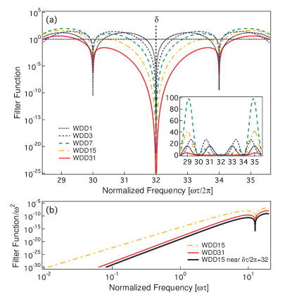
Figure 3: (color online) Noise suppression at fixed frequency. (a) Filter function about normalized frequency $\delta$ on a semilog scale for various WDD sequences, resulting in a notch where noise is suppressed. The notch bandwidth increases with sequency and the order of error suppression about $\delta$ increases with $r$. Inset: Same filter functions plotted on a linear scale. (b) Filter function normalized by $\omega^{2}$ for WDD15 and WDD31. The solid thick line shows WDD15 at $\delta/2\pi=2^{5}$, where the horizontal axis represents detuning from $\delta$. Here the order of error suppression as a function of detuning has increased by one order and is comparable to that for WDD31 near zero frequency. See text for details.

Such a zero may be realized in the filter function of the WDD sequence; from Sec. III.2, we recall that the filter function $F(\omega\tau)$ has a natural period (translational invariance, see Fig. 3) at $\tau_{\text{min}}/2\pi$, corresponding to $\tau/(2^{m+1}\pi)$. This produces the requisite zeroes in the filter function at fixed values of $\delta$, a feature intrinsic to the formulation of WDD.

In order to gain a quantitative understanding, let us calculate the Fourier transform of the sequence propagator,

$$\tilde{y}(\omega\tau)=\int_{0}^{\tau}dt\textsf{W}_{n}(t/\tau)e^{i(\delta+\Delta)t/\tau}.$$ (19)

We extract the filter function’s dependence on $\Delta$ near $\delta$ by use of an equality that is similar to Eq. (10),

$$\int_{0}^{1}dx\prod_{\left\{k\right\}}\textsf{R}_{k}\left(x\right)e^{i2^{r+1}\pi x}\sum_{i=0}^{r}a_{i}x^{i}=0,$$ (20)

where the set $\left\{k\right\}$ has $r$ elements in it, $k\geq 1$ and $\textrm{max}\left(k\right)\leq r$. A sketch of the proof of Eq. (20) appears in the Appendix. If the frequency $\delta/2\pi=2^{k}/\tau$, then Eq. (19) can be written as

$$\tilde{y}(\omega\tau)=\tau\int_{0}^{1}dt^{\prime}\prod_{\left\{k\right\}}\textsf{R}\left(k,t^{\prime}\right)e^{i2^{r+1}\pi t^{\prime}}\sum_{m=r+1}^{\infty}\frac{(i\Delta^{\prime}t^{\prime})^{m}}{m!},$$ (21)

where we have defined $t^{\prime}=t/\tau$ and $\Delta^{\prime}=\Delta\tau$. This expression indicates that $\tilde{y}(\omega\tau)$ scales like $\Delta^{r+1}$ in the vicinity of $\delta$. Thus, the slope of the rolloff as a function of detuning is set by $r$, giving increasing robustness to fluctuations in detuning from $\delta$. For fixed $r$, the bandwidth of the “notch” increases with sequency, as does the equivalent $\Omega_{p}$. These properties are expressed in Fig 3.

While the filter function is translationally symmetric, we see that the form of filter performance around $\delta$ is not the same as it is around $\omega=0$, due to the factor of $\omega^{-2}$ appearing in Eq. 2. An expansion as a function of $\Delta$ therefore yields improved performance relative to the zero-frequency rolloff when accounting for this factor.

It thus follows that for the specific case treated here by flipping the laser phase at times corresponding to the $\text{WDD}_{n}$, the error in the detuning $\delta$ can be suppressed up to order $r+1$, where as before $r$ is the Hamming weight of $n$. This general approach was studied experimentally in Ref. Hayes et al. (2011). Interestingly, this sequence can be interpreted as a high-order DCG where the primitive gates $Q$ are defined as $\tau_{\text{min}}$-long periods of evolution at detuning $\delta=2\pi/\tau_{\text{min}}$ and the $X$ gates are implemented by phase flips. We can interpret all the resulting DCGs generated by WDD sequences as repetitions and concatenations of the basic sequence $XQXQ$, resulting in a corrected gate $Q^{2^{m}}$ which is the desired entangling operation but has an error that scales with $\Delta^{2(r+1)}$.

V Benefits of WDD over other optimized approaches

Interest in the DD community has recently focused on optimized pulse sequences producing high-order suppression of noise either through analytical approaches (e.g. UDD Uhrig (2007)), numerical optimization (e.g. Locally Optimized ODD (LODD) Biercuk et al. (2009a), Optimized noise Filtration DD (OFDD) Uys et al. (2009), Bandwidth Adapted DD (BADD) Khodjasteh et al. (2011)), or combinations of optimization and concatenation strategies (e.g. concatenated UDD (CUDD) Uhrig (2009), QDD West et al. (2010), Nested UDD (NUDD) Wang and Liu (2011)). These sequences bring many benefits in terms of resource-efficient DD, as they generally optimize error-suppression against pulse number.

Studies have shown, however, that the extraordinary benefits provided by optimized sequences are largely suppressed in the presence of realistic constraints such as imperfect control pulses Biercuk et al. (2009b); Xiao et al. (2011); Wang and Dobrovitski (2010), digital clocking Biercuk et al. (2011), and timing limitations Hodgson et al. (2010). Moreover, noise suppression benefits have been shown to be minimal for $S_{\beta}(\omega)$ dominated by low-frequency noise and exhibiting slowly decaying high-frequency tails Uhrig (2008); Uys et al. (2009); Pasini and Uhrig (2010).

The WDD sequences possess benefits over existing approaches along two primary metrics:

$\bullet$ Efficient hardware sequencing;

$\bullet$ Restricted search space for sequencing.

We will separately explore each of these benefits next.

V.1 Efficient hardware sequencing

Current experiments in DD employ a user-programmed microprocessor and a complex hardware chain (e.g., a signal generator controlled by a programmable logic device responsible for pulse timing and under PC control). This is appropriate for demonstration experiments, but fails to provide a scalable solution due to both sequencing challenges and the difficulty of input-output (I/O) in complex or quantum systems. We are therefore interested in finding solutions permitting all sequence generation to be performed at the local level.

Once we accept this consideration, our metrics of efficiency change relative to the majority of published literature. When considering optimized DD, sequencing is complex and will likely require either a local microprocessor to decode instructions and apply a DD sequence, or multiple high-bandwidth communication pathways to external controllers. Both situations pose challenges in terms of significant local power dissipation in control hardware and energy inflows associated with I/O pathways. The energy expended in the number of pulses applied may contribute only a small amount of the total local power dissipation given these considerations. Given a presumed need for local DD sequence generation we thus arrive at digital sequencing complexity as the relevant metric for efficiency.

WDD meets this challenge, its primary benefit being that the Walsh functions are easily produced using simple digital circuits Beauchamp (1975). We identify Rademacher function generators (square-wave generators) as basic hardware resources for the physical-layer implementation of dynamical error suppression, realizing the control propagator in real-time. Rademacher functions may be generated in hardware with relative ease from a distributed clock signal, and may be added/multiplied together via hardware logic to generate Walsh toggling frames (for instance Harmuth’s array generator Beauchamp (1975)). The number of Rademacher functions required to achieve a given error suppression may therefore be deemed a relevant quantitative means of establishing the sequencing complexity.

As we have shown, a WDD sequence derived from $r$ Rademacher functions cancels the first $r-1$ orders of dephasing noise, and the sequences derived from $\textsf{W}_{2^{r}-1}(x)\equiv$ CDD_r do so for the smallest value of sequency (for fixed $r$). WDD therefore provides the highest-possible order of error suppression with respect to the number of Rademacher functions required to implement a given DD protocol, providing efficiency in the sequencing complexity. For the same sequencing complexity $r$, using sequences with different $n$ permits modification of $\Omega_{p}$, giving flexible control over noise filtering capabilities. By contrast, other optimized sequences discussed above require substantially greater sequencing resources, as the Walsh-transformation of a sequence such as UDD indicates the need for a large $r$ in order to generate the requisite $\{\delta_{j}\}$.

Furthermore, the structure of WDD and Walsh function generation is compatible with a nested or concatenated structure of decoupling about multiple axes, which enables the generation of GWDD sequences for generic decoherence. In the special case of a large separation of timescales for different decoherence processes, GWDD also allows for efficient bit-stacking of Walsh functions derived from similar hardware, but executed with different time-bases. Finally, we note that certain sequences constructed by recursively repeating the same base sequence many times may find value in circumstances where long-time storage and low-latency memory interrupts are desired in addition to improved low-frequency error suppression. This topic will be addressed in a separate manuscript.

Once a given Walsh function (or set of Walsh functions) is generated, conversion to WDD in real time may be achieved via hardware differentiation or edge-triggering of separate circuitry producing pre-programmed control pulses. Overall complexity is reduced by separating control sequencing from pulse generation.

Using Walsh functions for generation of the control propagator and hardware techniques for the triggering of applied pulses therefore provides a means to efficiently realize dynamical error suppression at the local level. Through this approach the need for access to a user-controlled microprocessor in order to send pulse-sequence commands to hardware, or for a local processor to interpret externally generated commands may be obviated: all control and timing may be performed using relatively simple digital logic realized in an Application Specific Integrated Circuit. A system protected by WDD sequences may run semi-autonomously, implementing pre-selected WDD sequences, or it may be programmed externally, where the only communicated information required could be the value of $n$ in binary (or as Gray code), a repetition number, and a trigger signal starting the sequence.

A significant challenge in such schemes is suppression of spurious rising/falling edge signals arising from, say, propagation delays in digital circuitry. However, latching WDD sequences to the clock signal should aid suppression of these signals. Accounting for nonzero-duration control pulses with $\tau_{\pi}$ an integer multiple of the clock period, may also be achieved through use of latching logic to introduce hardware delays while the control operations are applied. However, the effect of such delays on WDD performance would need to be characterized in detail. The creation of an optimized hardware-based generator of WDD sequences remains a problem for future study.

V.2 Restricted search space

While there already exists a plethora of DD procedures within the bang-bang limit, in practice not all these procedures will be suitable to the operating range of physical systems or the demands of quantum information processing protocols. This is true despite the fact that the objective in all such procedures is identical: maximize the fidelity of preserving an arbitrary quantum state for a desired time. For sufficiently simple experimental systems, an empirical optimization procedure (such as LODD) can sample over the space of all permissible DD pulse sequences and search for an optimal one. This idea has also been explored numerically in the above-mentioned OFDD and BADD protocols, as well in optimized DD for power-law spectra Pasini and Uhrig (2010). These approaches grow significantly in complexity as the pulse number increases, for instance in a large scale system requiring long-term storage. The central idea in WDD – that sequences using digital timing are made by attaching or repeating smaller sequences recursively – can be instrumental in significantly reducing the search space for finding optimal DD sequences empirically or numerically. We briefly outline potential implications of this idea here.

The canonical model of single-qubit dephasing with a given noise power spectral density used through most of this paper retains considerable structure in choosing when to apply the $X$ pulses. This persists even when enforcing digital timing conditions as below. Given $N=2^{m}$ time-bins, each of duration $\tau_{\text{min}}$, one may elect to either apply or not apply a pulse, thus generating a space of $2^{N}=2^{2^{m}}=2^{2^{\tau/\tau_{\text{min}}}}$ possible sequences. Performing a complete search over this space becomes extremely challenging as the total duration $\tau$ of the DD procedure grows, as observed in numerical approaches to generating randomized DD protocols Santos and Viola (2006, 2008) and to optimized sequences Biercuk et al. (2009a); Uys et al. (2009).

WDD provides a natural means to reduce the search space for the generation of dynamical error suppression sequences as there are only $N=2^{m}=2^{\tau/\tau_{\text{min}}}$ WDD sequences within the operational constraints of the problem. It also provides an intuitive analytical framework allowing pre-selection of certain sequences within WDD, further reducing the search space. For instance, a search might exclude all WDD sequences with $r<r_{\text{min}}$, as they will be known to provide insufficient low-frequency noise suppression. With such constraints, and the relative simplicity of implementing WDD in hardware, these sequences become especially attractive for an empirical search in which the performance of each sequence is tested in an actual experimental setting.

Perhaps even more interesting are the options offered when Walsh DD is extended to generic decoherence of a larger set of qubits in a quantum memory. Recently, an efficient perturbative DD procedure for this task has been explored (NUDD) that utilizes $(D_{S}^{2})^{r}$ pulses for $r$th order decoupling of a generic $D_{S}=2^{n_{q}}$-dimensional system of $n_{q}$ qubits Wang and Liu (2011). This procedure assumes the most general form of errors, including many-body errors. However, in reality error models are generally sparse. A fundamental problem of DD of many qubit systems (closely related to quantum simulation algorithms Wocjan et al. (2002); Leung (2002); Rötteler (2008)) is to optimize the decoupling when the error model for the interaction of the qubits is locally sparse. Using the procedure described in Sec. IV.2, we can progressively produce a search space for such an optimization procedure starting from elements of a basic DD sequence and recursively building longer sequences by the WDD construction procedure (repetition/concatenation).

VI Conclusion

In this manuscript we have studied the problem of reducing sequencing complexity in a dynamical error suppression framework, through consideration of digital modulation schemes. Towards this end we have introduced the Walsh functions as a mathematical basis for the generation of dynamical error suppression sequences. We have revealed how Walsh dynamical decoupling naturally incorporates familiar sequences (e.g. PDD, CPMG, CDD), and examined the properties of all the possible recursively structured sequences corresponding to Walsh functions.

Our analysis has demonstrated that the order of error suppression achieved by a given WDD sequence is set by the number of elementary Rademacher functions required to generate that sequence. This is manifested as a scaling of the low-frequency rolloff in the filter function as $6(r+1)$ dB/octave, with $r$ the number of Rademacher functions appearing in the sequence. Meanwhile, the high-frequency performance of a WDD sequence, and hence its noise-suppression bandwidth, is tunable via selection of $n$ for a given $r$, providing significant flexibility in sequence construction. Further we have introduced a simple means to construct WDD sequences using concatenation and repetition, and a technique to suppress general errors via GWDD.

We have shown that the Walsh functions provide efficient performance against control complexity, quantified by the value of $r$, and the supporting sequencing hardware. We believe that sequencing complexity will serve as a useful new metric with significant weight in system-level analyses, going far beyond standard optimization over pulse number in a DD sequence.

These considerations are likely to make the Walsh functions an attractive framework for the development of a quantum memory incorporating hardware-efficient physical-layer error-suppression strategies. Interestingly, the problem of searching for (digital) DD sequences with high order error suppression properties is also related to finding Littewood complex polynomials with high order zeroes Byrnes and Newman (1988); Berend and Golan (2006), which may point to further connections with both signal processing theory and polynomial analysis and approximation. From a practical standpoint, the variety of WDD sequences realizable through simple hardware sequencing provides a flexible solution for many future experimental systems.

Appendix A Order of error suppression

In this section we prove that for a given Paley ordering $r$, as long as $i\leq r$:

$$\int_{0}^{1}\textsf{R}_{1}(x)\cdots\textsf{R}_{j_{r+1}}(x)x^{i}dx=0,$$ (22)

where $j_{k}$ are non-zero positive integers in increasing order. This identity can be used to show the error suppression of the WDD sequences directly in the time domain and can be mathematically interpreted as the vanishing of the moments of the Walsh functions on the unit interval.

We proceed by induction on $r$ starting with the base case, $r=0$:

$$\int_{0}^{1}\textsf{R}_{j_{1}}(x)dx=0.$$ (23)

Since $j_{1}>0$, the corresponding Rademacher function $\textsf{R}_{j_{1}}$ will be periodic and balanced on $[0,1]$, which validates the base case in Eq. (23).

For the inductive step, let us assume that

$$\int_{0}^{1}\textsf{R}_{j_{1}}(x)...\textsf{R}_{j_{r+1}}(x)x^{i}dx=0,$$ (24)

where $i\leq r$. We need to prove that

$$\int_{0}^{1}\textsf{R}_{j_{1}}\left(x\right)...\textsf{R}_{j_{r+1}}(x)\textsf{R}_{j_{r+2}}(x)x^{i}dx=0,$$ (25)

where $i\leq r+1$.

The sign of Rademacher function $\textsf{R}_{j}(x)$ is determined by the $j$-th binary digit of $x$ which we refer to as $b_{j}(x)$. When $i=0$, Eq. (25) reduces to the average (zeroth moment) of the product of Rademacher functions over the interval $[0,1]$. We give a probabilistic argument for the cancellation of this average which can also be proven using induction. The average of the product of the Rademacher functions can be written as

$$\int_{0}^{1}(-1)^{b_{j_{1}}(x)}\cdots(-1)^{b_{j_{r+2}}(x)}dx.$$ (26)

We can interpret the above integral as an expectation value (denoted below by $E$) of a function of a real random variable $x$ distributed uniformly over the interval $[0,1]$. The corresponding (Lebesgue) probability measure $dx$ is equivalent to products of independent and uniform (discrete) measures for each binary digit of $x$ Adams and Guillemin (1996). We can thus rewrite Eq. (26) in the form

$$E[(-1)^{b_{j_{1}}}\cdots(-1)^{b_{j_{r+2}}}]=E[(-1)^{b_{j_{1}}}]\cdots E[(-1)^{b_{j_{r+2}}}]=0.$$

We can then use the $i=0$ case as the base for another induction proof over $i$, where we assume that Eq. (25) holds for all $i^{\prime}\leq r$. We refer to this as the “inner induction” assumption and proceed to prove Eq. (25) for $i=r+1$, which we rewrite as

$$I=\int_{0}^{1}\textsf{W}_{n}(x)\textsf{R}_{j_{1}}\left(x\right)x^{r+1}dx.$$ (27)

Note that we have singled out the lowest order Rademacher function in the product and written the product of the rest as a Walsh function with Paley ordering $n$. We can rewrite the integral as

$$I=\Big{(}\int_{0}^{2^{-j_{1}}}\!-\int_{2^{-j_{1}}}^{2\times 2^{-j_{1}}}\!+\int_{2\times 2^{-j_{1}}}^{3\times 2^{-j_{1}}}\!-\cdots\Big{)}\textsf{W}_{n}(x)x^{r+1}dx,$$

where the integrals match the positive and negative values of the Rademacher function $\textsf{R}_{j_{1}}$. Making the substitution $x^{\prime}=x-2^{-j_{1}}$ for the negative-signed terms, we can write

$$I=\Big{(}\int_{0}^{2^{-j_{1}}}\!+\int_{2\times 2^{-j_{1}}}^{3\times 2^{-j_{1}}}\!+\cdots\Big{)}[x^{r+1}\textsf{W}_{n}(x)-(x+2^{-j_{1}})^{r+1}\textsf{W}_{n}(x+2^{-j_{1}})]dx.$$ (28)

The Walsh function $\textsf{W}_{n}$ is constructed entirely of Rademacher functions with indices larger than $j_{1}$ having periods that commensurate with $2^{-j_{1}}$, which results in $\textsf{W}_{n}(x+2^{-j_{1}})=\textsf{W}_{n}(x)$. This allows us to write

$$I=\Big{(}\int_{0}^{2^{-j_{1}}}\!+\int_{2\times 2^{-j_{1}}}^{3\times 2^{-j_{1}}}\!+\cdots\Big{)}\textsf{W}_{n}(x)[x^{r+1}-(x+2^{-j_{1}})^{r+1}]dx.$$ (29)

We can rewrite the above as an integral over $[0,1]$ using the kernel $(\textsf{R}_{j_{1}}(x)+1)/2$:

$$I=\int_{0}^{1}\textsf{W}_{n}(x)\frac{\textsf{R}_{j_{1}}(x)+1}{2}[x^{r+1}-(x+2^{-j_{1}+1})^{r+1}]dx,$$

where the leading $x^{r+1}$ powers cancel when we expand $(x+2^{-j_{1}+1})^{r+1}$, leaving us with an integrand in which every power of $x$ appears with an exponent $i^{\prime}$ less than or equal to $r$. This matches the assumptions of our inner induction, leading to the cancellation of the integral for $i={r+1}$ and thus establishing the main result in Eq. (22).

We also note the following result, related to the WDD filter function at higher frequencies and used in Sec. IV.3 of the main text:

$$\int_{0}^{1}\textsf{R}_{1}(x)\cdots\textsf{R}_{j_{r}}(x)e^{i2^{r+1}\pi x}x^{i}dx=0,$$ (30)

where $i\leq r$ and we have used the highest Rademacher function in the product with a trigonometric function of the same period. This result can also be proven by induction in a similar manner.

It is interesting to note that the only properties of the Rademacher functions that are used in our proof are their “frequencies” and symmetry. Thus, any family of functions that mimics the periods and the sign changes of the Rademacher function family could in principle be used in our proof.