Optimally sparse approximations of 3D functions by compactly supported shearlet frames

Abstract

We study efficient and reliable methods of capturing and sparsely representing anisotropic structures in 3D data. As a model class for multidimensional data with anisotropic features, we introduce generalized three-dimensional cartoon-like images. This function class will have two smoothness parameters: one parameter $\beta$ controlling classical smoothness and one parameter $\alpha$ controlling anisotropic smoothness. The class then consists of piecewise $C^{\beta}$-smooth functions with discontinuities on a piecewise $C^{\alpha}$-smooth surface. We introduce a pyramid-adapted, hybrid shearlet system for the three-dimensional setting and construct frames for $L^{2}(\mathbb{R}^{3})$ with this particular shearlet structure. For the smoothness range $1<\alpha\leq\beta\leq 2$ we show that pyramid-adapted shearlet systems provide a nearly optimally sparse approximation rate within the generalized cartoon-like image model class measured by means of non-linear $N$-term approximations.

1 Introduction

Recent advances in modern technology have created a new world of huge, multi-dimensional data. In biomedical imaging, seismic imaging, astronomical imaging, computer vision, and video processing, the capabilities of modern computers and high-precision measuring devices have generated 2D, 3D and even higher dimensional data sets of sizes that were infeasible just a few years ago. The need to efficiently handle such diverse types and huge amounts of data has initiated an intense study in developing efficient multivariate encoding methodologies in the applied harmonic analysis research community. In neuro-imaging, e.g., fluorescence microscopy scans of living cells, the discontinuity curves and surfaces of the data are important specific features since one often wants to distinguish between the image “objects” and the “background”, e.g., to distinguish actin filaments in eukaryotic cells; that is, it is important to precisely capture the edges of these 1D and 2D structures. This specific application is an illustration that important classes of multivariate problems are governed by anisotropic features. The anisotropic structures can be distinguished by location and orientation or direction which indicates that our way of analyzing and representing the data should capture not only location, but also directional information. This is exactly the idea behind so-called directional representation systems which by now are well developed and understood for the 2D setting. Since much of the data acquired in, e.g., neuro-imaging, are truly three-dimensional, analyzing such data should be performed by three-dimensional directional representation systems. Hence, in this paper, we therefore aim for the 3D setting.

In applied harmonic analysis the data is typically modeled in a continuum setting as square-integrable functions or distributions. In dimension two, to analyze the ability of representation systems to reliably capture and sparsely represent anisotropic structures, Candés and Donoho [7] introduced the model situation of so-called cartoon-like images, i.e., two-dimensional functions which are piecewise $C^{2}$-smooth apart from a piecewise $C^{2}$ discontinuity curve. Within this model class there is an optimal sparse approximation rate one can obtain for a large class of non-adaptive and adaptive representation systems. Intuitively, one should think adaptive systems would be far superior in this task, but it has been shown in recent years that non-adaptive methods using curvelets, contourlets, and shearlets all have the ability to essentially optimal sparsely approximate cartoon-like images in 2D measured by the $L^{2}$-error of the best $N$-term approximation [7, 17, 13, 24].

1.1 Dimension three

In the present paper we will consider sparse approximations of cartoon-like images using shearlets in dimension three. The step from the one-dimensional setting to the two-dimensional setting is necessary for the appearance of anisotropic features at all. When further passing from the two-dimensional setting to the three-dimensional setting, the complexity of anisotropic structures changes significantly. In 2D one “only” has to handle one type of anisotropic features, namely curves, whereas in 3D one has to handle two geometrically very different anisotropic structures: Curves as one-dimensional features and surfaces as two-dimensional anisotropic features. Moreover, the analysis of sparse approximations in dimension two depends heavily on reducing the analysis to affine subspaces of $\mathbb{R}^{2}$. Clearly, these subspaces always have dimension and co-dimension one in 2D. In dimension three, however, we have subspaces of co-dimension one and two, and one therefore needs to perform the analysis on subspaces of the “correct” co-dimension. Therefore, the 3D analysis requires fundamental new ideas.

Finally, we remark that even though the present paper only deals with the construction of shearlet frames for $L^{2}(\mathbb{R}^{3})$ and sparse approximations of such, it also illustrates how many of the problems that arises when passing to higher dimensions can be handled. Hence, once it is known how to handle anisotropic features of different dimensions in 3D, the step from 3D to 4D can be dealt with in a similar way as also the extension to even higher dimensions. Therefore the extension of the presented result in $L^{2}(\mathbb{R}^{3})$ to higher dimensions $L^{2}(\mathbb{R}^{n})$ should be, if not straightforward, then at least be achievable by the methodologies developed.

1.2 Modelling anisotropic features

The class of 2D cartoon-like images consists, as mentioned above, of piecewise $C^{2}$-smooth functions with discontinuities on a piecewise $C^{2}$-smooth curve, and this class has been investigated in a number of recent publications. The obvious extension to the 3D setting is to consider functions of three variables being piecewise $C^{2}$-smooth function with discontinuities on a piecewise $C^{2}$-smooth surface. In some applications the $C^{2}$-smoothness requirement is too strict, and we will, therefore, go one step further and consider a larger class of images also containing less regular images. The generalized class of cartoon-like images in 3D considered in this paper consists of three-dimensional piecewise $C^{\beta}$-smooth functions with discontinuities on a piecewise $C^{\alpha}$ surface for $\alpha\in\left({1},{2}\right]$. Clearly, this model provides us with two new smoothness parameters: $\beta$ being a classical smoothness parameter and $\alpha$ being an anisotropic smoothness parameter, see Figure 1 for an illustration.

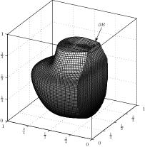
Figure 1: The support of a 3D cartoon-like image $f=f_{0}\chi_{B}$, where $f_{0}$ is $C^{\beta}$ smooth with $\mathop{\operator@font supp}\nolimits f_{0}=\mathbb{R}^{3}$ and the discontinuity surface $\partial B$ is piecewise $C^{\alpha}$ smooth.

This image class is unfortunately not a linear space as traditional smoothness spaces, e.g., Hölder, Besov, or Sobolev spaces, but it allows one to study the quality of the performance of representation systems with respect to capturing anisotropic features, something that is not possible with traditional smoothness spaces.

Finally, we mention that allowing piecewise $C^{\alpha}$-smoothness and not everywhere $C^{\alpha}$-smoothness is an essential way to model singularities along surfaces as well as along curves which we already described as the two fundamental types of anisotropic phenomena in 3D.

1.3 Measure for Sparse Approximation and Optimality

The quality of the performance of a representation system with respect to cartoon-like images is typically measured by taking a non-linear approximation viewpoint. More precisely, given a cartoon-like image and a representation system, the chosen measure is the asymptotic behavior of the $L^{2}$ error of $N$-term (non-linear) approximations in the number of terms $N$. When the anisotropic smoothness $\alpha$ is bounded by the classical smoothness as $\alpha\leq\frac{4}{3}\beta$, the anisotropic smoothness of the cartoon-like images will be the determining factor for the optimal approximation error rate one can obtain. To be more precise, as we will show in Section 3, the optimal approximation rate for the generalized 3D cartoon-like images models $f$ which can be achieved for a large class of adaptive and non-adaptive representation systems for $1<\alpha\leq\beta\leq 2$ is

$$\left\lVert f-f_{N}\right\rVert_{L^{2}}^{2}\leq C\cdot N^{-\alpha/2}\qquad\text{as }N\to\infty,$$

for some constant $C>0$, where $f_{N}$ is an $N$-term approximation of $f$. For cartoon-like images, wavelet and Fourier methods will typically have an $N$-term approximation error rate decaying as $N^{-1/2}$ and $N^{-1/3}$ as $N\to\infty$, respectively, see [23]. Hence, as the anisotropic smoothness parameter $\alpha$ grows, the approximation quality of traditional tools becomes increasingly inferior as they will deliver approximation error rates that are far from the optimal rate $N^{-\alpha/2}$. Therefore, it is desirable and necessary to search for new representation systems that can provide us with representations with a more optimal rate. This is where pyramid-adapted, hybrid shearlet systems enter the scene. As we will see in Section 6, this type of representation system provides nearly optimally sparse approximations:

$$\left\lVert f-f_{N}\right\rVert_{L^{2}}^{2}\leq\left\{\begin{aligned} C\cdot N^{-\alpha/2+\tau},&\qquad\text{if }\beta\in\left[{\alpha},{2}\right),\\ C\cdot N^{-1}(\log{N})^{2},&\qquad\text{if }\beta=\alpha=2,\end{aligned}\right\}\quad\text{ as $N\to\infty$,}$$

where $f_{N}$ is the $N$-term approximation obtained by keeping the $N$ largest shearlet coefficients, and $\tau=\tau(\alpha)$ with $0\leq\tau<0.04$ and $\tau\to 0$ for $\alpha\to 1^{+}$ and for $\alpha\to 2^{-}$. Clearly, the obtained sparse approximations for these shearlet systems are not truly optimal owing to the polynomial factor $\tau$ for $\alpha<2$ and the polylog factor for $\alpha=2$. On the other hand, it still shows that non-adaptive schemes such as the hybrid shearlet system can provide rates that are nearly optimal within a large class of adaptive and non-adaptive methods.

1.4 Construction of 3D hybrid shearlets

Shearlet theory has become a central tool in analyzing and representing 2D data with anisotropic features. Shearlet systems are systems of functions generated by one single generator with parabolic scaling, shearing, and translation operators applied to it, in much the same way wavelet systems are dyadic scalings and translations of a single function, but including a directionality characteristic owing to the additional shearing operation and the anisotropic scaling. Of the many directional representation systems proposed in the last decade, e.g., steerable pyramid transform [29], directional filter banks [3], 2D directional wavelets [2], curvelets [6], contourlets [13], bandelets [28], the shearlet system [25] is among the most versatile and successful. The reason for this being an extensive list of desirable properties: Shearlet systems can be generated by one function, they precisely resolve wavefront sets, they allow compactly supported analyzing elements, they are associated with fast decomposition algorithms, and they provide a unified treatment of the continuum and the digital realm. We refer to [22] for a detailed review of the advantages and disadvantages of shearlet systems as opposed to other directional representation systems.

Several constructions of discrete band-limited and compactly supported 2D shearlet frames are already known, see [15, 21, 9, 26, 20, 11]; for construction of 3D shearlet frames less is known. Dahlke, Steidl, and Teschke [10] recently generalized the shearlet group and the associated continuous shearlet transform to higher dimensions $\mathbb{R}^{n}$. Furthermore, in [10] they showed that, for certain band-limited generators, the continuous shearlet transform is able to identify hyperplane and tetrahedron singularities. Since this transform originates from a unitary group representation, it is not able to capture all directions, in particular, it will not capture the delta distribution on the $x_{1}$-axis (and more generally, any singularity with “$x_{1}$-directions”). We will use a different tiling of the frequency space, namely systems adapted to pyramids in frequency space, to avoid this non-uniformity of directions. We call these systems pyramid-adapted shearlet system[22]. In [16], the continuous version of the pyramid-adapted shearlet system was introduced, and it was shown that the location and the local orientation of the boundary set of certain three-dimensional solid regions can be precisely identified by this continuous shearlet transform. Finally, we will also need to use a different scaling than the one from [10] in order to achieve shearlet systems that provide almost optimally sparse approximations.

Since spatial localization of the analyzing elements of the encoding system is very important both for a precise detection of geometric features as well as for a fast decomposition algorithm, we will mainly follow the sufficient conditions for and construction of compactly supported cone-adapted 2D shearlets by Kittipoom and two of the authors [20] and extend these result to the 3D setting (Section 4). These results provide us with a large class of separable, compactly supported shearlet systems with “good” frame bounds, optimally sparse approximation properties, and associated numerically stable algorithms. One important new aspect is that dilation will depend on the smoothness parameter $\alpha$. This will provide us with hybrid shearlet systems ranging from classical parabolic based shearlet systems ($\alpha=2$) to almost classical wavelet systems ($\alpha\approx 1$). In other words, we obtain a parametrized family of shearlets with a smooth transition from (nearly) wavelets to shearlets. This will allow us to adjust our shearlet system according to the anisotropic smoothness of the data at hand. For rational values of $\alpha$ we can associate this hybrid system with a fast decomposition algorithm using the fast Fourier transform with multiplication and periodization in the frequency space (in place of convolution and down-sampling).

Our compactly supported 3D hybrid shearlet elements (introduced in Section 4) will in the spatial domain be of size $2^{-j\alpha/2}$ times $2^{-j/2}$ times $2^{-j/2}$ for some fixed anisotropy parameter $1<\alpha\leq 2$. When $\alpha\approx 1$ this corresponds to “cube-like” (or “wavelet-like”) elements. As $\alpha$ approaches $2$ the scaling becomes less and less $isotropic$ yielding “plate-like” elements as $j\to\infty$. This indicates that these anisotropic 3D shearlet systems have been designed to efficiently capture two-dimensional anisotropic structures, but neglecting one-dimensional structures. Nonetheless, these 3D shearlet systems still perform optimally when representing and analyzing cartoon-like functions that have discontinuities on piecewise $C^{\alpha}$-smooth surfaces – as mentioned such functions model 3D data that contain both point, curve, and surface singularities.

Let us end this subsection with a general thought on the construction of band-limited tight shearlet frames versus compactly supported shearlet frames. There seem to be a trade-off between compact support of the shearlet generators, tightness of the associated frame, and separability of the shearlet generators. The known constructions of tight shearlet frames, even in 2D, do not use separable generators, and these constructions can be shown to not be applicable to compactly supported generators. Moreover, these tight frames use a modified version of the pyramid-adapted shearlet system in which not all elements are dilates, shears, and translations of a single function. Tightness is difficult to obtain while allowing for compactly supported generators, but we can gain separability as in Theorem 10 hence fast algorithmic realizations. On the other hand, when allowing non-compactly supported generators, tightness is possible, but separability seems to be out of reach, which makes fast algorithmic realizations very difficult.

1.5 Other approaches for 3D data

Other directional representation systems have been considered for the 3D setting. We mention curvelets [5, 4], surflets [8], and surfacelets [27]. This line of research is mostly concerned with constructions of such systems and not their sparse approximation properties with respect to cartoon-like images. In [8], however, the authors consider adaptive approximations of Horizon class function using surflet dictionaries which generalizes the wedgelet dictionary for 2D signals to higher dimensions.

During the final stages of this project, we realized that a similar almost optimal sparsity result for the 3D setting (for the model case $\alpha=\beta=2$) was reported by Guo and Labate [18] using band-limited shearlet tight frames. They provide a proof for the case where the discontinuity surface is (non-piecewise) $C^{2}$-smooth using the X-ray transform.

1.6 Outline

We give the precise definition of generalized cartoon-like image model class in Section 2, and the optimal rate of approximation within this model is then derived in Section 3. In Section 4 and Section 5 we construct the so-called pyramid-adapted shearlet frames with compactly supported generators. In Sections 6 to 9 we then prove that such shearlet systems indeed deliver nearly optimal sparse approximations of three-dimensional cartoon-like images. We extend this result to the situation of discontinuity surfaces which are piecewise $C^{\alpha}$-smooth except for zero- and one-dimensional singularities and again derive essential optimal sparsity of the constructed shearlet frames in Section 10. We end the paper by discussion various possible extensions in Section 11.

1.7 Notation

We end this introduction by reviewing some basic definitions. The following definitions will mostly be used for the case $n=3$, but they will however be defined for general $n\in\mathbb{N}$. For $x\in\mathbb{R}^{n}$ we denote the $p$-norm on $\mathbb{R}^{n}$ of $x$ by $\left\lVert x\right\rVert_{p}$. The Lebesgue measure on $\mathbb{R}^{n}$ is denoted by $\left\lvert\cdot\right\rvert$ and the counting measure by $\#\left\lvert\cdot\right\rvert$. Sets in $\mathbb{R}^{n}$ are either considered equal if they are equal up to sets of measure zero or if they are element-wise equal; it will always be clear from the context which definition is used. The $L^{p}$-norm of $f\in L^{p}(\mathbb{R}^{n})$ is denoted by $\left\lVert f\right\rVert_{L^{p}}$. For $f\in L^{1}(\mathbb{R}^{n})$, the Fourier transform is defined by

$$\hat{f}(\xi)=\int_{\mathbb{R}^{n}}f(x)\,\mathrm{e}^{-2\pi i\left\langle\xi,x\right\rangle_{\!}}\,\mathrm{d}x$$

with the usual extension to $L^{2}(\mathbb{R}^{n})$. The Sobolev space and norm are defined as

$$H^{s}(\mathbb{R}^{n})=\left\{{f\colon\mathbb{R}^{n}\to\mathbb{C}}:{\left\lVert f\right\rVert_{H^{s}}^{2}:=\int_{\mathbb{R}^{n}}\big{(}1+|\xi|^{2}\big{)}^{s}\big{|}\hat{f}(\xi)\big{|}^{2}\,\mathrm{d}\xi<+\infty}\right\}.$$

For functions $f:\mathbb{R}^{n}\to\mathbb{C}$ the homogeneous Hölder seminorm is given by

$$\left\lVert f\right\rVert_{\dot{C}^{\beta}}:=\max_{\left\lvert\gamma\right\rvert=\left\lfloor\beta\right\rfloor}\;\sup_{x,x^{\prime}\in\mathbb{R}^{n}}\frac{\left\lvert\partial^{\gamma}f(x)-\partial^{\gamma}f(x^{\prime})\right\rvert}{\left\lVert x-x^{\prime}\right\rVert_{2}^{\{\beta\}}},$$

where $\{\beta\}=\beta-\left\lfloor\beta\right\rfloor$ is the fractional part of $\beta$ and $\left\lvert\gamma\right\rvert$ is the usual length of a multi-index $\gamma=(\gamma_{1},\gamma_{2},\dots,\gamma_{n})$. Further, we let

$$\left\lVert f\right\rVert_{{C}^{\beta}}:=\max_{\gamma\leq\left\lfloor\beta\right\rfloor}\sup{\left\lvert\partial^{\gamma}f\right\rvert}+\left\lVert f\right\rVert_{\dot{C}^{\beta}},$$

and we denote by $C^{\beta}(\mathbb{R}^{n})$ the space of Hölder functions, i.e., functions $f:\mathbb{R}^{n}\to\mathbb{C}$, whose $C^{\beta}$-norm is bounded.

2 Generalized 3D cartoon-like image model class

The first complete model of 2D cartoon-like images was introduced in [7], the basic idea being that a closed $C^{2}$-curve separates two $C^{2}$-smooth functions. For 3D cartoon-like images we consider square integrable functions of three variables that are piecewise $C^{\beta}$-smooth with discontinuities on a piecewise $C^{\alpha}$-smooth surface.

Fix $\alpha>0$ and $\beta>0$, and let $\rho:\left[{0},{2\pi}\right)\times\left[{0},{\pi}\right]\to\left[{0},{\infty}\right)$ be continuous and define the set $B$ in $\mathbb{R}^{3}$ by

$$B=\{x\in\mathbb{R}^{3}:\left\lVert x\right\rVert_{2}\leq\rho(\theta_{1},\theta_{2}),x=(\left\lVert x\right\rVert_{2},\theta_{1},\theta_{2})\text{ in spherical coordinates}\}.$$

We require that the boundary $\partial B$ of $B$ is a closed surface parametrized by

$$b(\theta_{1},\theta_{2})=\begin{pmatrix}\rho(\theta_{1},\theta_{2})\cos(\theta_{1})\sin(\theta_{2})\\ \rho(\theta_{1},\theta_{2})\sin(\theta_{1})\sin(\theta_{2})\\ \rho(\theta_{1},\theta_{2})\cos(\theta_{2})\end{pmatrix},\quad\theta=(\theta_{1},\theta_{2})\in\left[{0},{2\pi}\right)\times\left[{0},{\pi}\right].$$ (1)

Furthermore, the radius function $\rho$ must be Hölder continuous with coefficient $\nu$, i.e.,

$$\left\lVert\rho\right\rVert_{\dot{C}^{\alpha}}=\max_{\left\lvert\gamma\right\rvert=\left\lfloor\alpha\right\rfloor}\;\sup_{\theta,\theta^{\prime}}\frac{\left\lvert\partial^{\gamma}\rho(\theta)-\partial^{\gamma}\rho(\theta^{\prime})\right\rvert}{\left\lVert\theta-\theta^{\prime}\right\rVert_{2}^{\{\alpha\}}}\leq\nu,\quad\rho=\rho(\theta_{1},\theta_{2}),\quad\rho\leq\rho_{0}<1.$$ (2)

For $\nu>0$, the set $\mathit{STAR}^{\alpha}(\nu)$ is defined to be the set of all $B\subset\left[{0},{1}\right]^{3}$ such that $B$ is a translate of a set obeying (1) and (2). The boundary of the surfaces in $\mathit{STAR}^{\alpha}(\nu)$ will be the discontinuity sets of our cartoon-like images. We remark that any starshaped sets in $\left[{0},{1}\right]^{3}$ with bounded principal curvatures will belong to $\mathit{STAR}^{2}(\nu)$ for some $\nu$. Actually, the property that the sets in $\mathit{STAR}^{\alpha}(\nu)$ are parametrized by spherical angles, which implies that the sets are starshaped, is not important to us. For $\alpha=2$ we could, e.g., extend $\mathit{STAR}^{2}(\nu)$ to be all bounded subset of $\left[{0},{1}\right]^{3}$, whose boundary is a closed $C^{2}$ surface with principal curvatures bounded by $\nu$.

To allow more general discontinuities surfaces, we extend $\mathit{STAR}^{\alpha}(\nu)$ to a class of sets $B$ with piecewise $C^{\alpha}$ boundaries $\partial B$. We denote this class $\mathit{STAR}^{\alpha}(\nu,L)$, where $L\in\mathbb{N}$ is the number of $C^{\alpha}$ pieces and $\nu>0$ be an upper bound for the “curvature” on each piece. In other words, we say that $B\in\mathit{STAR}^{\alpha}(\nu,L)$ if $B$ is a bounded subset of $\left[{0},{1}\right]^{3}$ whose boundary $\partial B$ is a union of finitely many pieces $\partial B_{1},\dots,\partial B_{L}$ which do not overlap except at their boundaries, and each patch $\partial B_{i}$ can be represented in parametric form $\rho_{l}=\rho_{l}(\theta_{1},\theta_{2})$ by a $C^{\alpha}$-smooth radius function with $\left\lVert\rho_{l}\right\rVert_{\dot{C}^{\alpha}}\leq\nu$. We remark that we put no restrictions on how the patches $\partial B_{l}$ meet, in particular, $B\in\mathit{STAR}^{\alpha}(\nu,L)$ can have arbitrarily sharp edges joining the pieces $\partial B_{l}$. Also note that $\mathit{STAR}^{\alpha}(\nu)=\mathit{STAR}^{\alpha}(\nu,1)$.

The actual objects of interest to us are, as mentioned, not these starshaped sets, but functions that have the boundary $\partial B$ as discontinuity surface.

Definition 1.

Let $\nu,\mu>0$, $\alpha,\beta\in\left({1},{2}\right]$, and $L\in\mathbb{N}$. Then ${\mathcal{E}}^{\beta}_{\alpha,L}(\mathbb{R}^{3})$ denotes the set of functions $f:\mathbb{R}^{3}\to\mathbb{C}$ of the form

$$f=f_{0}+f_{1}\chi_{B},$$

where $B\in\mathit{STAR}^{\alpha}(\nu,L)$ and $f_{i}\in C^{\beta}(\mathbb{R}^{3})$ with $\mathop{\operator@font supp}\nolimits f_{0}\subset\left[{0},{1}\right]^{3}$ and $\left\lVert f_{i}\right\rVert_{C^{\beta}}\leq\mu$ for each $i=0,1$. We let ${\mathcal{E}}^{\beta}_{\alpha}(\mathbb{R}^{3}):={\mathcal{E}}^{\beta}_{\alpha,1}(\mathbb{R}^{3})$.

We speak of ${\mathcal{E}}^{\beta}_{\alpha,L}(\mathbb{R}^{3})$ as consisting of cartoon-like 3D images having $C^{\beta}$-smoothness apart from a piecewise $C^{\alpha}$ discontinuity surface. We stress that ${\mathcal{E}}_{\alpha,L}^{\beta}(\mathbb{R}^{3})$ is not a linear space of functions and that ${\mathcal{E}}^{\beta}_{\alpha,L}(\mathbb{R}^{3})$ depends on the constants $\nu$ and $\mu$ even though we suppress this in the notation. Finally, we let ${\mathcal{E}}_{\alpha,L}^{\text{bin}}(\mathbb{R}^{3})$ denote binary cartoon-like images, that is, functions $f=f_{0}+f_{1}\chi_{B}\in{\mathcal{E}}_{\alpha,L}^{\beta}(\mathbb{R}^{3})$, where $f_{0}=0$ and $f_{1}=1$.

3 Optimality bound for sparse approximations

After having clarified the model situation ${\mathcal{E}}^{\beta}_{\alpha,L}(\mathbb{R}^{3})$, we will now discuss which measure for the accuracy of approximation by representation systems we choose, and what optimality means in this case. We will later in Section 6 restrict the parameter range in our model class ${\mathcal{E}}^{\beta}_{\alpha,L}(\mathbb{R}^{3})$ to $1<\alpha\leq\beta\leq 2$. In this section, however, we will find the theoretical optimal approximation error rate within ${\mathcal{E}}^{\beta}_{\alpha,L}(\mathbb{R}^{3})$ for the full range $1<\alpha\leq 2$ and $\beta\geq 0$. Before we state and prove the main optimal sparsity result of this section, Theorem 3, we discuss the notions of $N$-term approximations and frames.

3.1 $N$-term approximations

Let $\Phi=\left\{{\phi_{i}}\right\}_{i\in I}$ be a dictionary with the index set $I$ not necessarily being countable. We seek to approximate each single element of ${\mathcal{E}}^{\beta}_{\alpha,L}(\mathbb{R}^{3})$ with elements from $\Phi$ by $N$ terms of this system. For this, let $f\in{\mathcal{E}}^{\beta}_{\alpha,L}(\mathbb{R}^{3})$ be arbitrarily chosen. Letting now $N\in\mathbb{N}$, we consider $N$-term approximations of $f$, i.e.,

$$\sum_{i\in{I}_{N}}{c}_{i}\phi_{i}\quad\text{with }{I}_{N}\subset I,\,\#\left\lvert{I}_{N}\right\rvert=N.$$

The best $N$-term approximation to $f$ is an $N$-term approximation

$$f_{N}=\sum_{i\in{I}_{N}}{c}_{i}\phi_{i},$$

which satisfies that, for all $I_{N}\subset I$, $\#\left\lvert I_{N}\right\rvert=N$, and for all scalars $(c_{i})_{i\in I}$,

$$\left\lVert f-f_{N}\right\rVert_{L^{2}}\leq\Bigl{\lVert}f-\sum_{i\in I_{N}}c_{i}\phi_{i}\Bigr{\rVert}_{L^{2}}.$$

3.2 Frames

A frame for a separable Hilbert space $\mathcal{H}$ is a countable collection of vectors $\{f_{j}\}_{j\in\mathbb{J}}$ for which there are constants $0<A\leq B<\infty$ such that

$$A\left\lVert f\right\rVert^{2}\leq\sum_{j\in\mathbb{J}}\left\lvert\left\langle f,f_{j}\right\rangle_{\!}\right\rvert^{2}\leq B\left\lVert f\right\rVert^{2}\qquad\text{for all }f\in\mathcal{H}.$$

If the upper bound in this inequality holds, then $\{f_{j}\}_{j\in\mathbb{J}}$ is said to be a Bessel sequence with Bessel constant $B$. For a Bessel sequence $\{f_{j}\}_{j\in\mathbb{J}}$, we define the frame operator of $\{f_{j}\}_{j\in\mathbb{J}}$ by

$$S\colon\mathcal{H}\to\mathcal{H},\qquad Sf=\sum_{j\in\mathbb{J}}\left\langle f,f_{j}\right\rangle_{\!}f_{j}.$$

If $\{f_{j}\}_{j\in\mathbb{J}}$ is a frame, this operator is bounded, invertible, and positive. A frame $\{f_{j}\}_{j\in\mathbb{J}}$ is said to be tight if we can choose $A=B$. If furthermore $A=B=1$, the sequence $\{f_{j}\}_{j\in\mathbb{J}}$ is said to be a Parseval frame. Two Bessel sequences $\{f_{j}\}_{j\in\mathbb{J}}$ and $\{g_{j}\}_{j\in\mathbb{J}}$ are said to be dual frames if

$$f=\sum_{j\in\mathbb{J}}\left\langle f,g_{j}\right\rangle_{\!}f_{j}\qquad\text{for all }f\in\mathcal{H}.$$

It can be shown that, in this case, both Bessel sequences are even frames, and we shall say that the frame $\{g_{j}\}_{j\in\mathbb{J}}$ is dual to $\{f_{j}\}_{j\in\mathbb{J}}$, and vice versa. At least one dual always exists; it is given by $\{S^{-1}f_{j}\}_{j\in\mathbb{J}}$ and called the canonical dual.

Now, suppose the dictionary $\Phi$ forms a frame for $L^{2}(\mathbb{R}^{3})$ with frame bounds $A$ and $B$, and let $\{{\tilde{\phi}_{i}}\}_{i\in I}$ denote the canonical dual frame. We then consider the expansion of $f$ in terms of this dual frame, i.e.,

$$f=\sum_{i\in I}\langle f,\phi_{i}\rangle\tilde{\phi}_{i}.$$

For any $f\in L^{2}(\mathbb{R}^{2})$ we have $(\left\langle f,\phi_{i}\right\rangle_{\!})_{i\in I}\in\ell^{2}(I)$ by definition. Since we only consider expansions of functions $f$ belonging to a subset ${\mathcal{E}}^{\beta}_{\alpha,L}(\mathbb{R}^{3})$ of $L^{2}(\mathbb{R}^{3})$, this can, at least, potentially improve the decay rate of the coefficients so that they belong to $\ell^{p}(I)$ for some $p<2$. This is exactly what is understood by sparse approximation (also called compressible approximations). We hence aim to analyze shearlets with respect to this behavior, i.e., the decay rate of shearlet coefficients.

For frames, tight and non-tight, it is not possible to derive a usable, explicit form for the best $N$-term approximation. We therefore crudely approximate the best $N$-term approximation by choosing the $N$-term approximation provided by the indices ${I}_{N}$ associated with the $N$ largest coefficients $\langle f,\phi_{i}\rangle$ in magnitude with these coefficients, i.e.,

$$f_{N}=\sum_{i\in{I}_{N}}\langle f,\phi_{i}\rangle\tilde{\phi}_{i}.$$

However, even with this rather crude greedy selection procedure, we obtain very strong results for the approximation rate of shearlets as we will see in Section 6.

The following well-known result shows how the $N$-term approximation error can be bounded by the tail of the square of the coefficients $c_{i}=\left\langle f,\phi_{i}\right\rangle_{\!}$. We refer to [23] for a proof.

Lemma 2.

Let $\{{\phi_{i}}\}_{i\in I}$ be a frame for $H$ with frame bounds $A$ and $B$, and let $\{{\tilde{\phi}_{i}}\}_{i\in I}$ be the canonical dual frame. Let $I_{N}\subset I$ with $\#\left\lvert I_{N}\right\rvert=N$, and let $f_{N}$ be the $N$-term approximation $f_{N}=\sum_{i\in I_{N}}\left\langle f,\phi_{i}\right\rangle_{\!}\tilde{\phi}_{i}$. Then

$$\left\lVert f-f_{N}\right\rVert^{2}\leq\frac{1}{A}\sum_{i\notin I_{N}}\left\lvert\left\langle f,\phi_{i}\right\rangle_{\!}\right\rvert^{2}$$

for any $f\in L^{2}(\mathbb{R}^{3})$.

Let $c^{\ast}$ denote the non-increasing (in modulus) rearrangement of $c=(c_{i})_{i\in I}=(\left\langle f,\phi_{i}\right\rangle_{\!})_{i\in I}$, e.g., $c^{\ast}_{\,n}$ denotes the $n$th largest coefficient of $c$ in modulus. This rearrangement corresponds to a bijection $\pi:\mathbb{N}\to I$ that satisfies

$$\pi:\mathbb{N}\to I,\quad c_{\pi(n)}=c^{\ast}_{\,n}\text{ for all $n\in\mathbb{N}$}.$$

Since $c\in\ell^{2}(I)$, also $c^{\ast}\in\ell^{2}(\mathbb{N})$. Let $f$ be a cartoon-like image, and suppose that $\left\lvert c^{\ast}_{n}\right\rvert$, in this case, even decays as

$$\left\lvert c^{\ast}_{n}\right\rvert\lesssim n^{-(\alpha+2)/4}\qquad\text{for}\quad n\to\infty$$ (3)

for some $\alpha>0$, where the notation $h(n)\lesssim g(n)$ means that there exists a $C>0$ such that $h(n)\leq Cg(n)$, i.e., $h(n)=O(g(n))$. Clearly, we then have $c^{\ast}\in\ell^{p}(\mathbb{N})$ for $p\geq\tfrac{4}{\alpha+2}$. By Lemma 2, the $N$-term approximation error will therefore decay as

$$\left\lVert f-f_{N}\right\rVert^{2}\leq\frac{1}{A}\sum_{n>N}\left\lvert c^{\ast}_{n}\right\rvert^{2}\lesssim\sum_{n>N}n^{-\alpha/2+1}\asymp N^{-\alpha/2},$$ (4)

where $f_{N}$ is the $N$-term approximation of $f$ by keeping the $N$ largest coefficients, that is,

$$f_{N}=\sum_{n=1}^{N}c^{*}_{\,n}\,\tilde{\phi}_{\pi(n)}.$$ (5)

The notation $h(n)\asymp g(n)$, sometimes also written as $h(n)=\Theta(g(n))$, used above means that $h$ is bounded both above and below by $g$ asymptotically as $n\to\infty$, that is, $h(n)=O(g(n))$ and $g(n)=O(h(n))$. The approximation error rate $N^{-\alpha/2}$ obtained in (4) is exactly the sought optimal rate mentioned in the introduction. This illustrates that the fraction $\frac{\alpha+2}{4}$ introduced in the decay of the sequence $c^{*}$ will play a major role in the following. In particular, we are searching for a representation system $\Phi$ which forms a frame and delivers decay of $c=(\left\langle f,\phi_{i}\right\rangle_{\!})_{i\in I}$ as in (3) for any cartoon-like image.

3.3 Optimal sparsity

In this subsection we will state and prove the main result of this section, Theorem 3, but let us first discuss some of its implications for sparse approximations of cartoon-like images.

From the $\Phi=\{{\phi_{i}}\}_{i\in I}$ dictionary with the index set $I$ not necessarily being countable, we consider expansions of the form

$$f=\sum_{i\in I_{f}}c_{i}\,\phi_{i},$$ (6)

where $I_{f}\subset I$ is a countable selection from $I$ that may depend on $f$. Moreover, we can assume that $\phi_{i}$ are normalized by $\left\lVert\phi_{i}\right\rVert_{L^{2}}=1$. The selection of the $i$th term is obtained according to a selection rule $\sigma(i,f)$ which may adaptively depend on $f$. Actually, the $i$th element may also be modified adaptively and depend on the first $(i-1)$th chosen elements [14]. We assume that how deep or how far down in the indexed dictionary $\Phi$ we are allowed to search for the next element $\phi_{i}$ in the approximation is limited by a polynomial $\pi$. Without such a depth search limit, one could choose $\Phi$ to be a countable, dense subset of $L^{2}(\mathbb{R}^{3})$ which would yield arbitrarily good sparse approximations, but also infeasible approximations in practise. We shall denote any sequence of coefficients $c_{i}$ chosen according to these restrictions by $c(f)=(c(f)_{i})_{i}$.

We are now ready to state the main result of this section. Following Donoho [14] we say that a function class $\mathcal{F}$ contains an embedded orthogonal hypercube of dimension $m$ and side $\delta$ if there exists $f_{0}\in\mathcal{F}$, and orthogonal functions $\psi_{i,m,\delta}$, $i=1,\dots,m$, with $\left\lVert\psi_{i,m,\delta}\right\rVert_{L^{2}}=\delta$, such that the collection of hypercube vertices

$$\mathcal{H}(m;f_{0},\{\psi_{i}\}):=\left\{{f_{0}+\sum_{i=1}^{m}\xi_{i}\psi_{i,m,\delta}}:{\xi_{i}\in\{0,1\}}\right\}$$

is contained in $\mathcal{F}$. The sought bound on the optimal sparsity within the set of cartoon-like images will be obtained by showing that the cartoon-like image class contains sufficiently high-dimensional hypercubes with sufficiently large sidelength; intuitively, we will see that a certain high complexity of the set of cartoon-like images limits the possible sparsity level. The meaning of “sufficiently” is made precise by the following definition. We say that a function class $\mathcal{F}$ contains a copy of $\ell^{p}_{0}$ if $\mathcal{F}$ contains embedded orthogonal hypercubes of dimension $m(\delta)$ and side $\delta$, and if, for some sequence $\delta_{k}\to 0$, and some constant $C>0$:

$$m(\delta_{k})\geq C\,\delta_{k}^{-p},\qquad k=k_{0},k_{0}+1,\dots$$ (7)

The first part of the following result is an extension from the 2D to the 3D setting of [14, Thm. 3].

Theorem 3.

1. The class of binary cartoon-like images ${\mathcal{E}}_{\alpha}^{\text{bin}}(\mathbb{R}^{3})$ contains a copy of $\ell^{p}_{0}$ for $p=4/(\alpha+2)$.

2. The space of Hölder functions $C^{\beta}(\mathbb{R}^{3})$ with compact support in $\left[{0},{1}\right]^{3}$ contains a copy of $\ell^{p}_{0}$ for $p=6/(2\beta+3)$.

Before providing a proof of the theorem, let us discuss some of its implications for sparse approximations of cartoon-like images. Theorem 3(i) implies, by [14, Theorem 2], that for every $p<4/(\alpha+2)$ and every method of atomic decomposition based on polynomial $\pi$ depth search from any countable dictionary $\Phi$, we have for $f\in{\mathcal{E}}_{\alpha}^{\text{bin}}(\mathbb{R}^{3})$:

$$\min_{\sigma(n,f)\leq\pi(n)}\max_{f\in{\mathcal{E}}_{\alpha,L}^{\beta}(\mathbb{R}^{3})}\left\lVert c(f)\right\rVert_{w\ell^{p}}=+\infty,$$ (8)

where the weak-$\ell_{p}$ “norm” is defined as $\left\lVert c(f)\right\rVert_{w\ell^{p}}=\sup_{n>0}n^{1/p}\left\lvert c^{*}_{\,n}\right\rvert$. Sparse approximations are approximations of the form $\sum_{i}c(f)_{i}\,\phi_{i}$ with coefficients $c(f)_{n}^{\ast}$ decaying at certain, hopefully high, rate. Equation (8) is a precise statement of the optimal achievable sparsity level. No representation system (up to the restrictions described above) can deliver expansions (6) for ${\mathcal{E}}^{\text{bin}}_{\alpha}(\mathbb{R}^{3})$ with coefficients satisfying $c(f)\in w\ell_{p}$ for $p<4/(\alpha+2)$. As we will see in Theorems 13 and 14, pyramid-adapted shearlet frames deliver $(\left\langle f,\psi_{\lambda}\right\rangle_{\!})_{\lambda}\in w\ell^{p}$ for $p=4/(\alpha+2-2\tau)$, where $0\leq\tau<0.04$.

Assume for a moment that we have an “optimal” dictionary $\Phi$ at hand that delivers $c(f)\in w\ell^{4/(\alpha+2)}$, and assume further that it is also a frame. As we saw in the Section 3.2, this implies that

$$\left\lVert f-f_{N}\right\rVert_{L^{2}}^{2}\lesssim N^{-\alpha/2}\qquad\text{as }N\to\infty,$$

where $f_{N}$ is the $N$-term approximation of $f$ by keeping the $N$ largest coefficients. Therefore, no frame representation system can deliver at better approximation error rate than $O(N^{-\alpha/2})$ under the chosen approximation procedure within the image model class ${\mathcal{E}}_{\alpha}^{\text{bin}}(\mathbb{R}^{3})$. If $\Phi$ is actually an orthonormal basis, then this is truly the optimal rate since best $N$-term approximations, in this case, are obtained by keeping the $N$ largest coefficients.

Similarly, Theorem 3(ii) tells us that the optimal approximation error rate within the Hölder function class is $O(N^{-2\beta/3})$. Combining the two estimates we see that the optimal approximation error rate within the full cartoon-like image class ${\mathcal{E}}^{\beta}_{\alpha}(\mathbb{R}^{3})$ cannot exceed $O(N^{-\min\{\alpha/2,2\beta/3\}})$ convergence. For the parameter range $1<\alpha\leq\beta\leq 2$, this rate reduces to $O(N^{-\alpha/2})$. For $\alpha=\beta=2$, as will show in Section 6, shearlet systems actually deliver this rate except from an additional polylog factor, namely $O(N^{-\alpha/2}(\log N)^{2})=O(N^{-1}(\log N)^{2})$. For $1<\alpha\leq\beta\leq 2$ and $\alpha<2$, the $\log$-factor is replaced by a small polynomial factor $N^{\tau(\alpha)}$, where $\tau(\alpha)<0.04$ and $\tau(\alpha)\to 0$ for $\alpha\to 1^{+}$ or $\alpha\to 2^{-}$.

It is striking that one is able to obtain such a near optimal approximation error rate since the shearlet system as well as the approximation procedure will be non-adaptive; in particular, since traditional, non-adaptive representation systems such as Fourier series and wavelet systems are far from providing an almost optimal approximation rate. This is illustrated in the following example.

Example 1.

Let $B=B(x,\rho)$ be the ball in $\left[{0},{1}\right]^{3}$ with center $x$ and radius $r$. Define $f=\chi_{B}$. Clearly, $f\in{\mathcal{E}}^{2}_{2}(\mathbb{R}^{3})$ if $B\subset\left[{0},{1}\right]^{3}$. Suppose $\Phi=\{{\mathrm{e}^{2\pi ikx}}\}_{k\in\mathbb{Z}^{d}}$. The best $N$-term Fourier sum $f_{N}$ yields

$$\left\lVert f-f_{N}\right\rVert_{L^{2}}^{2}\asymp N^{-1/3}\qquad\text{for }N\to\infty,$$

which is far from the optimal rate $N^{-1}$. For the wavelet case the situation is only slightly better. Suppose $\Phi$ is any compactly supported wavelet basis. Then

$$\left\lVert f-f_{N}\right\rVert_{L^{2}}^{2}\asymp N^{-1/2}\qquad\text{for }N\to\infty,$$

where $f_{N}$ is the best $N$-term approximation from $\Phi$. The calculations leading to these estimates are not difficult, and we refer to [23] for the details. We will later see that shearlet frames yield $\left\lVert f-f_{N}\right\rVert_{L^{2}}^{2}\lesssim N^{-1}(\log N)^{2}$, where $f_{N}$ is the best $N$-term approximation.

We mention that the rates obtained in Example 1 are typical in the sense that most cartoon-like images will yield the exact same (and far from optimal) rates.

Finally, we end the subsection with a proof of Theorem 3.

Proof of Theorem 3.

The idea behind the proofs is to construct a collection of functions in ${\mathcal{E}}_{\alpha}^{\text{bin}}(\mathbb{R}^{3})$ and $C^{\beta}(\mathbb{R}^{3})$, respectively, such that the collection of functions will be vertices of a hypercube with dimension satisfying (7).

(i): Let $\varphi_{1}$ and $\varphi_{2}$ be smooth $C^{\infty}$ functions with compact support $\mathop{\operator@font supp}\nolimits\varphi_{1}\subset\left[{0},{2\pi}\right]$ and $\mathop{\operator@font supp}\nolimits\varphi_{2}\subset\left[{0},{\pi}\right]$. For $A>0$ and $m\in\mathbb{N}$ we define:

$$\varphi_{i,m}(t)=\varphi_{i_{1},i_{2},m}(t)=Am^{-\alpha}\varphi_{1}(mt_{1}-2\pi i_{1})\varphi_{2}(mt_{2}-\pi i_{2}),$$

for $i_{1},i_{2}\in\{0,\dots,m-1\}$, where $i=(i_{1},i_{2})$ and $t=(t_{1},t_{2})$. We let further $\varphi(t):=\varphi_{1}(t_{1})\varphi_{2}(t_{2})$. It is easy to see that $\left\lVert\varphi_{i,m}\right\rVert_{L^{1}}=m^{-\alpha+2}A\left\lVert\varphi\right\rVert_{L^{1}}$. Moreover, it can also be shown that $\left\lVert\varphi_{i,m}\right\rVert_{\dot{C}^{\alpha}}=A\left\lVert\varphi\right\rVert_{\dot{C}^{\alpha}}$, where $\left\lVert\cdot\right\rVert_{\dot{C}^{\alpha}}$ denotes the homogeneous Hölder norm introduced in (2).

Without loss of generality, we can consider the cartoon-like images ${\mathcal{E}}_{\alpha}^{\text{bin}}(\mathbb{R}^{3})$ translated by $-(\frac{1}{2},\frac{1}{2},\frac{1}{2})$ so that their support lies in $\left[{-1/2},{1/2}\right]^{3}$. Alternatively, we can fix an origin at $(1/2,1/2,1/2)$, and use spherical coordinates $(\rho,\theta_{1},\theta_{2})$ relative to this choice of origin. We set $\rho_{0}=1/4$ and define

$$\psi_{i,m}=\chi_{\{\rho_{0}<\rho\leq\rho_{0}+\varphi_{i,m}\}}\quad\text{for $i_{1},i_{2}\in\{0,\dots,m-1\}$}.$$

The radius functions $\rho_{\gamma}$ for $\gamma=(\gamma_{i_{1},i_{2}})_{i_{1},i_{2}\in\{{0,\dots,m-1}\}}$ with $\gamma_{i_{1},i_{2}}\in\{0,1\}$ defined by

$$\rho_{\gamma}(\theta_{1},\theta_{2})=\rho_{0}+\sum^{m}_{i_{1}=1}\sum^{m}_{i_{2}=1}\gamma_{i_{1},i_{2}}\,\varphi_{i,m}(\theta_{1},\theta_{2}),$$ (9)

determines the discontinuity surfaces of the functions of the form:

$$f_{\gamma}=\chi_{\{\rho\leq\rho_{0}\}}+\sum^{m}_{i_{1}=1}\sum^{m}_{i_{2}=1}\gamma_{i_{1},i_{2}}\psi_{i,m}\quad\text{for $\gamma_{i_{1},i_{2}}\in\{0,1\}$}.$$

For a fixed $m$ the functions $\psi_{i,m}$ are disjointly supported and therefore mutually orthogonal. Hence, ${\mathcal{H}}(m^{2},\chi_{\{\rho\leq\rho_{0}\}},\{\psi_{i,m}\})$ is a collection of hypercube vertices. Moreover,

$$\left\lVert\psi_{i,m}\right\rVert_{L^{2}}^{2} =\lambda(\left\{{(\rho,\theta_{1},\theta_{2})}:{\rho_{0}\leq\rho\leq\rho_{0}+\varphi_{i,m}(\theta_{1},\theta_{2})}\right\})$$

$$\leq\int_{0}^{2\pi}\int_{0}^{\pi}\int_{\rho_{0}}^{\rho_{0}+\varphi_{i,m}(\theta_{1},\theta_{2})}\rho^{2}\sin\theta_{2}\;d\rho\,d\theta_{2}\,d\theta_{1}$$

$$\leq C_{0}\,m^{-\alpha-2}\left\lVert\varphi\right\rVert_{L^{1}},$$

where the constant $C_{0}$ only depends on $A$. Any radius function $\rho=\rho(\theta_{1},\theta_{2})$ of the form (9) satisfies

$$\left\lVert\rho_{\gamma}\right\rVert_{\dot{C}^{\alpha}}\leq\left\lVert\varphi_{i,m}\right\rVert_{\dot{C}^{\alpha}}=A\left\lVert\varphi\right\rVert_{\dot{C}^{\alpha}}.$$

Therefore, $\left\lVert\rho\right\rVert_{\dot{C}^{\alpha}}\leq\nu$ whenever $A\leq\nu/\left\lVert\varphi\right\rVert_{\dot{C}^{\alpha}}$. This shows that we have the hypercube embedding

$${\mathcal{H}}(m^{2},\chi_{\{\rho\leq\rho_{0}\}},\{\psi_{i,m}\})\subset{\mathcal{E}}_{\alpha}^{\text{bin}}(\mathbb{R}^{3}).$$

The side length $\delta=\left\lVert\psi_{i,m}\right\rVert_{L^{2}}$ of the hypercube satisfies

$$\delta^{2}\leq C_{0}\,m^{-\alpha-2}\left\lVert\varphi\right\rVert_{L^{1}}\leq\nu\,\frac{\left\lVert\varphi\right\rVert_{L^{1}}}{\left\lVert\varphi\right\rVert_{\dot{C}^{\alpha}}}\,m^{-\alpha-2},$$

whenever $C_{0}\leq\nu/\left\lVert\varphi\right\rVert_{\dot{C}^{\alpha}}$. Now, we finally choose $m$ and $A$ as

$$m(\delta)=\left\lfloor\left(\frac{\delta^{2}}{\nu}\frac{\left\lVert\varphi\right\rVert_{\dot{C}^{\alpha}}}{\left\lVert\varphi\right\rVert_{L^{1}}}\right)^{-1/(\alpha+2)}\right\rfloor\quad\text{and}\quad A(\delta,\nu)=\delta^{2}m^{\alpha+2}/\left\lVert\varphi\right\rVert_{L^{1}}.$$

By this choice, we have $C_{0}\leq\nu/\left\lVert\varphi\right\rVert_{\dot{C}^{\alpha}}$ for sufficiently small $\delta$. Hence, ${\mathcal{H}}$ is a hypercube of side length $\delta$ and dimension $d=m(\delta)^{2}$ embedded in ${\mathcal{E}}_{\alpha}^{\text{bin}}(\mathbb{R}^{3})$. We obviously have $m(\delta)\geq C_{1}\nu^{\frac{1}{\alpha+2}}\delta^{-\frac{2}{\alpha+2}}$, thus the dimension $d$ of the hypercube obeys

$$d\geq C_{2}\,\delta^{-\frac{4}{\alpha+2}}$$

for all sufficiently small $\delta>0$.

(ii): Let $\varphi\in C_{0}^{\infty}(\mathbb{R})$ with compact support $\mathop{\operator@font supp}\nolimits\varphi\subset\left[{0},{1}\right]$. For $m\in\mathbb{N}$ to be determined, we define for $i_{1},i_{2},i_{3}\in\{0,\dots,m-1\}$:

$$\psi_{i,m}(t)=\psi_{i_{1},i_{2},i_{3},m}(t)=m^{-\beta}\varphi(mt_{1}-i_{1})\varphi(mt_{2}-i_{2})\varphi(mt_{3}-i_{3}),$$

where $i=(i_{1},i_{2},i_{3})$ and $t=(t_{1},t_{2},t_{3})$. We let $\psi(t):=\varphi(t_{1})\varphi(t_{2})\varphi(t_{3})$. It is easy to see that $\left\lVert\psi_{i,m}\right\rVert_{L^{2}}^{2}=m^{-2\beta-3}\left\lVert\psi\right\rVert_{L^{2}}^{2}$. We note that the functions $\psi_{i,m}$ are disjointly supported (for a fixed $m$) and therefore mutually orthogonal. Thus we have the hypercube embedding

$${\mathcal{H}}(m^{3},0,\{\psi_{i,m}\})\subset C^{\beta}(\mathbb{R}^{3}),$$

where the side length of the hypercube is $\delta=\left\lVert\psi_{i,m}\right\rVert_{L^{2}}=m^{-\beta-3/2}\left\lVert\psi\right\rVert_{L^{2}}$. Now, chose $m$ as

$$m(\delta)=\left\lfloor\left(\frac{\delta}{\left\lVert\psi\right\rVert_{L^{2}}}\right)^{-1/(\beta+3/2)}\right\rfloor.$$

Hence, ${\mathcal{H}}$ is a hypercube of side length $\delta$ and dimension $d=m(\delta)^{3}$ embedded in $C^{\beta}(\mathbb{R}^{3})$. The dimension $d$ of the hypercube obeys

$$d\geq C\,\delta^{-3\frac{1}{\beta+3/2}}=C\,\delta^{-\frac{6}{2\beta+3}},$$

for all sufficiently small $\delta>0$. ∎

3.4 Higher dimensions

Our main focus is, as mentioned above, the three-dimensional setting, but let us briefly sketch how the optimal sparsity result extends to higher dimensions. The $d$-dimensional cartoon-like image class ${\mathcal{E}}^{\beta}_{\alpha}(\mathbb{R}^{d})$ consists of functions having $C^{\beta}$-smoothness apart from a $(d-1)$-dimensional $C^{\alpha}$-smooth discontinuity surface. The $d$-dimensional analogue of Theorem 3 is then straightforward to prove.

Theorem 4.

1. The class of $d$-dimensional binary cartoon-like images ${\mathcal{E}}_{\alpha}^{\text{bin}}(\mathbb{R}^{d})$ contains a copy of $\ell^{p}_{0}$ for $p=2(d-1)/(\alpha+d-1)$.

2. The space of Hölder functions $C^{\beta}(\mathbb{R}^{d})$ contains a copy of $\ell^{p}_{0}$ for $p=\frac{2d}{2\beta+d}$.

It is then intriguing to analyze the behavior of $p=2(d-1)/(\alpha+d-1)$ and $p=2d/(2\beta+d)$. from Theorem 4. In fact, as $d\to\infty$, we observe that $p\to 2$ in both cases. Thus, the decay of any ${c(f)}$ for cartoon-like images becomes slower as $d$ grows and approaches $\ell^{2}$ which is actually the rate guaranteed for all $f\in L^{2}(\mathbb{R}^{d})$.

Moreover, by Theorem 4 we see that the optimal approximation error rate for $N$-term approximations $f_{N}$ within the class of $d$-dimensional cartoon-like images ${\mathcal{E}}^{\beta}_{\alpha}(\mathbb{R}^{d})$ is $N^{-\min\{\alpha/(d-1),2\beta/d\}}$. In this paper we will however restrict ourselves to the case $d=3$ since we, as mentioned in the introduction, can see this dimension as a critical one.

4 Hybrid shearlets in 3D

After we have set our benchmark for directional representation systems in the sense of stating an optimality criteria for sparse approximations of the cartoon-like image class ${\mathcal{E}}^{\beta}_{\alpha,L}(\mathbb{R}^{3})$, we next introduce the class of shearlet systems we claim behave optimally.

4.1 Pyramid-adapted shearlet systems

Fix $\alpha\in\left({1},{2}\right]$. We scale according to scaling matrices $A_{2^{j}}$, $\tilde{A}_{2^{j}}$ or $\breve{A}_{2^{j}}$, $j\in\mathbb{Z}$, and represent directionality by the shear matrices $S_{k}$, $\tilde{S}_{k}$, or $\breve{S}_{k}$, $k=(k_{1},k_{2})\in\mathbb{Z}^{2}$, defined by

$$A_{2^{j}} =\begin{pmatrix}2^{j\alpha/2}\!&0&0\\ 0&\!\!\!2^{j/2}\!&0\\ 0&0&\!\!\!2^{j/2}\end{pmatrix}\!, \tilde{A}_{2^{j}} = \begin{pmatrix}2^{j/2}&0&0\\ 0&\!\!\!2^{j\alpha/2}\!&0\\ 0&0&\!\!\!2^{j/2}\end{pmatrix}\!, \breve{A}_{2^{j}} = \begin{pmatrix}2^{j/2}\!&0&0\\ 0&\!\!\!2^{j/2}\!&0\\ 0&0&\!\!\!2^{j\alpha/2}\end{pmatrix},$$ and

and

$$S_{k} =\begin{pmatrix}1\;&k_{1}\;&k_{2}\\ 0&1&0\\ 0&0&1\end{pmatrix}, \tilde{S}_{k} = \begin{pmatrix}1&0&0\\ k_{1}\;&1\;&k_{2}\\ 0&0&1\end{pmatrix}, \breve{S}_{k}\; = \begin{pmatrix}1&0&0\\ 0&1&0\\ k_{1}\;&k_{2}\;&1\end{pmatrix},$$ and

respectively. The case $\alpha=2$ corresponds to paraboloidal scaling. As $\alpha$ decreases, the scaling becomes less anisotropic, and allowing $\alpha=1$ would yield isotropic scaling. The action of isotropic scaling and shearing is illustrated in Figure 2.

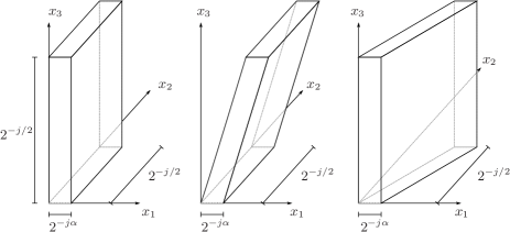
Figure 2: Sketch of the action of scaling ($\alpha\approx 2$) and shearing. For $\psi\in L^{2}(\mathbb{R}^{3})$ with $\mathop{\operator@font supp}\nolimits\psi\subset\left[{0},{1}\right]^{3}$ we plot the support of $\psi(S_{k}A_{j}\cdot)$ for fixed $j>0$ and various $k=(k_{1},k_{2})\in\mathbb{Z}^{2}$. From left to right: $k_{1}=k_{2}=0$, $k_{1}=0,k_{2}<0$, and $k_{1}<0,k_{2}=0$.

The translation lattices will be generated by the following matrices: $M_{c}=\mathrm{diag}(c_{1},c_{2},c_{2})$, $\tilde{M}_{c}=\mathrm{diag}(c_{2},c_{1},c_{2})$, and $\breve{M}_{c}=\mathrm{diag}(c_{2},c_{2},c_{1})$, where $c_{1}>0$ and $c_{2}>0$.

Figure 3: Sketch of the partition of the frequency domain. The centered cube ${\mathcal{C}}$ is shown, and the arrangement of the six pyramids is indicated by the “diagonal” lines. We refer to Figure 4 for a sketch of the pyramids.

We next partition the frequency domain into the following six pyramids:

$${\mathcal{P}}_{\iota}=\left\{\begin{array}[]{rcl}\{(\xi_{1},\xi_{2},\xi_{3})\in\mathbb{R}^{3}:\xi_{1}\geq 1,\,|\xi_{2}/\xi_{1}|\leq 1,\,|\xi_{3}/\xi_{1}|\leq 1\}&:&\iota=1,\\ \{(\xi_{1},\xi_{2},\xi_{3})\in\mathbb{R}^{3}:\xi_{2}\geq 1,\,|\xi_{1}/\xi_{2}|\leq 1,\,|\xi_{3}/\xi_{2}|\leq 1\}&:&\iota=2,\\ \{(\xi_{1},\xi_{2},\xi_{3})\in\mathbb{R}^{3}:\xi_{3}\geq 1,\,|\xi_{1}/\xi_{3}|\leq 1,\,|\xi_{2}/\xi_{3}|\leq 1\}&:&\iota=3,\\ \{(\xi_{1},\xi_{2},\xi_{3})\in\mathbb{R}^{3}:\xi_{1}\leq-1,\,|\xi_{2}/\xi_{1}|\leq 1,\,|\xi_{3}/\xi_{1}|\leq 1\}&:&\iota=4,\\ \{(\xi_{1},\xi_{2},\xi_{3})\in\mathbb{R}^{3}:\xi_{2}\leq-1,\,|\xi_{1}/\xi_{2}|\leq 1,\,|\xi_{3}/\xi_{2}|\leq 1\}&:&\iota=5,\\ \{(\xi_{1},\xi_{2},\xi_{3})\in\mathbb{R}^{3}:\xi_{3}\leq-1,\,|\xi_{1}/\xi_{3}|\leq 1,\,|\xi_{2}/\xi_{3}|\leq 1\}&:&\iota=6,\end{array}\right.$$

and a centered cube

$${\mathcal{C}}=\{(\xi_{1},\xi_{2},\xi_{3})\in\mathbb{R}^{3}:\left\lVert(\xi_{1},\xi_{2},\xi_{3})\right\rVert_{\infty}<1\}.$$

The partition is illustrated in Figures 3 and 4. This partition of the frequency space into pyramids allows us to restrict the range of the shear parameters. In case of the shearlet group systems, one must allow arbitrarily large shear parameters. For the pyramid-adapted systems, we can, however, restrict the shear parameters to $\left[{-\left\lceil 2^{j(\alpha-1)/2}\right\rceil},{\left\lceil 2^{j(\alpha-1)/2}\right\rceil}\right]$. We would like to emphasize that this approach is important for providing an almost uniform treatment of different directions – in a sense of a good approximation to rotation.

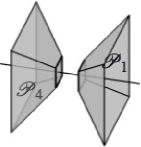
(a) Pyramids ${\mathcal{P}}_{1}$ and ${\mathcal{P}}_{4}$ and the $\xi_{1}$ axis.

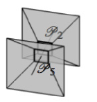
(b) Pyramids ${\mathcal{P}}_{2}$ and ${\mathcal{P}}_{5}$ and the $\xi_{2}$ axis.

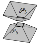
(c) Pyramids ${\mathcal{P}}_{3}$ and ${\mathcal{P}}_{6}$ and the $\xi_{3}$ axis.

Figure 4: The partition of the frequency domain: The “top” of the six pyramids.

These considerations are made precise in the following definition.

Definition 5.

For $\alpha\in\left({1},{2}\right]$ and $c=(c_{1},c_{2})\in(\mathbb{R}_{+})^{2}$, the pyramid-adapted, hybrid shearlet system $SH(\phi,\psi,\tilde{\psi},\breve{\psi};c,\alpha)$ generated by $\phi,\psi,\tilde{\psi},\breve{\psi}\in L^{2}(\mathbb{R}^{3})$ is defined by

$$SH(\phi,\psi,\tilde{\psi},\breve{\psi};c,\alpha)=\Phi(\phi;c_{1})\cup\Psi(\psi;c,\alpha)\cup\tilde{\Psi}(\tilde{\psi};c,\alpha)\cup\breve{\Psi}(\breve{\psi};c,\alpha),$$

where

$$\Phi(\phi;c_{1}) =\left\{{\phi_{m}=\phi(\cdot-m)}:{m\in c_{1}\mathbb{Z}^{3}}\right\},$$

$$\Psi(\psi;c,\alpha) =\left\{{\psi_{j,k,m}=2^{j\frac{\alpha+2}{4}}{\psi}({S}_{k}{A}_{2^{j}}\cdot-m)}:{j\geq 0,|k|\leq\lceil 2^{j(\alpha-1)/2}\rceil,m\in M_{c}\mathbb{Z}^{3}}\right\},$$

$$\tilde{\Psi}(\tilde{\psi};c,\alpha) =\{\tilde{\psi}_{j,k,m}=2^{j\frac{\alpha+2}{4}}\tilde{\psi}(\tilde{S}_{k}\tilde{A}_{2^{j}}\cdot-m):j\geq 0,|k|\leq\lceil 2^{j(\alpha-1)/2}\rceil,m\in\tilde{M}_{c}\mathbb{Z}^{3}\},$$

and

$$\breve{\Psi}(\breve{\psi};c,\alpha) =\{\breve{\psi}_{j,k,m}=2^{j\frac{\alpha+2}{4}}\breve{\psi}(\breve{S}_{k}\breve{A}_{2^{j}}\cdot-m):j\geq 0,|k|\leq\lceil 2^{j(\alpha-1)/2}\rceil,m\in\breve{M}_{c}\mathbb{Z}^{3}\},$$

where $j\in\mathbb{N}_{0}$ and $k\in\mathbb{Z}^{2}$. Here we have used the vector notation $\left\lvert k\right\rvert\leq K$ for $k=(k_{1},k_{2})$ and $K>0$ to denote $\left\lvert k_{1}\right\rvert\leq K$ and $\left\lvert k_{2}\right\rvert\leq K$. We will often use $\Psi(\psi)$ as shorthand notation for $\Psi(\psi;c,\alpha)$. If $SH(\phi,\psi,\tilde{\psi},\breve{\psi};c,\alpha)$ is a frame for $L^{2}(\mathbb{R}^{3})$, we refer to $\phi$ as a scaling function and $\psi$, $\tilde{\psi}$, and $\breve{\psi}$ as shearlets. Moreover, we often simply term $SH(\phi,\psi,\tilde{\psi},\breve{\psi};c,\alpha)$ pyramid-adapted shearlet system.

We let ${\mathcal{P}}={\mathcal{P}}_{1}\cup{\mathcal{P}}_{4}$, $\tilde{\mathcal{P}}={\mathcal{P}}_{2}\cup{\mathcal{P}}_{5}$, and $\breve{\mathcal{P}}={\mathcal{P}}_{3}\cup{\mathcal{P}}_{6}$. In the remainder of this paper, we shall mostly consider ${\mathcal{P}}$; the analysis for $\tilde{\mathcal{P}}$ and $\breve{\mathcal{P}}$ is similar (simply append $\tilde{\cdot}$ and $\breve{\cdot}$, respectively, to suitable symbols).

We will often assume the shearlets to be compactly supported in spatial domain. If e.g., $\mathop{\operator@font supp}\nolimits\psi\subset\left[{0},{1}\right]^{3}$, then the shearlet element $\psi_{j,k,m}$ will be supported in a parallelepiped with side lengths $2^{-j\alpha/2}$, $2^{-j/2}$, and $2^{-j/2}$, see Figure 2. For $\alpha=2$ this shows that the shearlet elements will become plate-like as $j\to\infty$. As $\alpha$ approaches $1$ the scaling becomes almost isotropic giving almost isotropic cube-like elements. The key fact to mind is, however, that our shearlet elements always become plate-like as $j\to\infty$ with aspect ratio depending on $\alpha$.

In general, however, we will have very weak requirements on the shearlet generators $\psi$, $\tilde{\psi}$, and $\breve{\psi}$. As a typical minimal requirement in our construction and approximation results we will require the shearlet $\psi$ to be feasible.

Definition 6.

Let $\delta,\gamma>0$. A function $\psi\in L^{2}(\mathbb{R}^{3})$ is called a $(\delta,\gamma)$-feasible shearlet associated with ${\mathcal{P}}$, if there exist $q\geq q^{\prime}>0$, $q\geq r>0$, $q\geq s>0$ such that

$$\lvert\hat{\psi}(\xi)\rvert\lesssim\min\{{1,\left\lvert q\xi_{1}\right\rvert^{\delta}}\}\;\min{\{{1,\left\lvert q^{\prime}\xi_{1}\right\rvert^{-\gamma}}\}}\;\min{\{{1,\left\lvert r\xi_{2}\right\rvert^{-\gamma}}\}}\;\min{\{{1,\left\lvert s\xi_{3}\right\rvert^{-\gamma}}\}},$$ (10)

for all $\xi=(\xi_{1},\xi_{2},\xi_{3})\in\mathbb{R}^{3}$. For the sake of brevity, we will often simply say that $\psi$ is $(\delta,\gamma)$-feasible.

Let us briefly comment on the decay assumptions in (10). If $\psi$ is compactly supported, then $\hat{\psi}$ will be a continuous function satisfying the decay assumptions as $\left\lvert\xi\right\rvert\to\infty$ for sufficiently small $\gamma>0$. The decay condition controlled by $\delta$ can be seen as a vanishing moment condition in the $x_{1}$-direction which suggests that a $(\delta,\gamma)$-feasible shearlet will behave as a wavelet in the $x_{1}$-direction.

5 Construction of compactly supported shearlets

In the following subsection we will describe the construction of pyramid-adapted shearlet systems with compactly supported generators. This construction uses ideas from the classical construction of wavelet frames in [12, §3.3.2]; we also refer to the recent construction of cone-adapted shearlet systems in $L^{2}(\mathbb{R}^{2})$ described in the paper [20].

5.1 Covering properties

We fix $\alpha\in\left({1},{2}\right]$, and let $\psi\in L^{2}(\mathbb{R}^{3})$ be a feasible shearlet associated with ${\mathcal{P}}$. We then define the function $\Phi:{\mathcal{P}}\times\mathbb{R}^{3}\to\mathbb{R}$ by

$$\Phi(\xi,\omega)=\sum_{j\geq 0}\sum_{k\leq\lceil 2^{j(\alpha-1)/2}\rceil}\left\lvert\hat{\psi}(S_{-k}^{T}A_{2^{-j}}\xi)\right\rvert\left\lvert\hat{\psi}(S_{-k}^{T}A_{2^{-j}}\xi+\omega)\right\rvert.$$ (11)

This function measures to which extent the effective part of the supports of the scaled and sheared versions of the shearlet generator overlaps. Moreover, it is linked to the so-called $t_{q}$-equations albeit with absolute value of the functions in the sum (11). We also introduce the function $\Gamma:\mathbb{R}^{3}\to\mathbb{R}$ defined by

$$\Gamma(\omega)=\operatorname*{ess\,sup}_{\xi\in{\mathcal{P}}}\Phi(\xi,\omega),$$

measuring the maximal extent to which these scaled and sheared versions overlap for a given distance $\omega\in\mathbb{R}^{3}$. The values

$$L_{\mathit{inf}}=\operatorname*{ess\,inf}_{\xi\in{\mathcal{P}}}\Phi(\xi,0)\qquad\text{and}\qquad L_{\mathit{sup}}=\operatorname*{ess\,sup}_{\xi\in{\mathcal{P}}}\Phi(\xi,0),$$ (12)

will relate to the classical discrete Calderón condition. Finally, the value

$$R(c)=\sum\limits_{m\in\mathbb{Z}^{3}\setminus\{0\}}\left[\Gamma\left({M_{c}^{-1}{m}}\right)\Gamma\left({-M_{c}^{-1}{m}}\right)\right]^{1/2},\quad\text{where}\quad c=(c_{1},c_{2})\in\mathbb{R}_{+}^{2},$$ (13)

measures the average of the symmetrized function values $\Gamma(M_{c}^{-1}m)$ and is again related to the so-called $t_{q}$-equations.

We now first turn our attention to the terms $L_{\mathit{sup}}$ and $R(c)$ and provide upper bounds for those. These estimates will later be used for estimates for frame bounds associated to a shearlet system; we remark that the to be derived estimates (15) and (17) also hold when the essential supremum in the definition of $L_{\mathit{sup}}$ and $R(c)$ is taken over all $\xi\in\mathbb{R}^{3}$.

To estimate the effect of shearing, we will repeatedly use the following estimates:

$$\sup_{(x,y)\in\mathbb{R}^{2}}\sum_{k\in\mathbb{Z}}\min\left\{{1,\left\lvert y\right\rvert}\right\}\min\left\{{1,\left\lvert x+ky\right\rvert^{-\gamma}}\right\}\leq 3+\frac{2}{\gamma-1}=:C(\gamma)$$ (14)

and

$$\sup_{(x,y)\in\mathbb{R}^{2}}\sum_{k\neq 0}\min\left\{{1,\left\lvert y\right\rvert}\right\}\min\left\{{1,\left\lvert x+ky\right\rvert^{-\gamma}}\right\}\leq 2+\frac{2}{\gamma-1}=C(\gamma)-1$$

for $\gamma>1$.

Proposition 7.

Suppose $\psi\in L^{2}(\mathbb{R}^{3})$ is a $(\delta,\gamma)$-feasible shearlet with $\delta>1$ and $\gamma>1/2$. Then

$$L_{\mathit{sup}}\leq\frac{q^{2}}{rs}\,C(2\gamma)^{2}\,\Bigl{(}\frac{1}{1-2^{(-\delta+1)\alpha}}+\left\lceil\frac{2}{\alpha}\log_{2}\Bigl{(}\frac{q}{q^{\prime}}\Bigr{)}\right\rceil+1\Bigr{)}<\infty,$$ (15)

where $C(\gamma)=3+\frac{2}{\gamma-1}$.

Proof.

By (10), we immediately have the following bound for $\Phi(\xi,0)$:

$$\Phi(\xi,0) \leq\sup_{\xi\in\mathbb{R}^{3}}\sum_{j\geq 0}\min{\bigl{\{}{1,|q2^{-j\alpha/2}\xi_{1}|^{2\delta}}\bigr{\}}}\;\min\bigl{\{}{1,|q^{\prime}2^{-j\alpha/2}\xi_{1}|^{-2\gamma}}\bigr{\}}$$

$$\phantom{\leq\sup\sum\;}\cdot\sum_{k_{1}\in\mathbb{Z}}\min\bigl{\{}{1,|r(2^{-j/2}\xi_{2}+k_{1}2^{-j\alpha/2}\xi_{1})|^{-2\gamma}}\bigr{\}}$$

$$\phantom{\leq\sup\sum\;}\cdot\sum_{k_{2}\in\mathbb{Z}}\min\bigl{\{}{1,|s(2^{-j/2}\xi_{3}+k_{2}2^{-j\alpha/2}\xi_{1})|^{-2\gamma}}\bigr{\}}.$$

Letting $\eta_{1}=q\xi_{1}$ and using that $q\geq r$ and $q\geq s$, we obtain

$$\Phi(\xi,0)\leq\sup_{(\eta_{1},\xi_{2},\xi_{3})\in\mathbb{R}^{3}}\sum_{j\geq 0}\min{\bigl{\{}{1,\bigl{\lvert}2^{-j\alpha/2}\eta_{1}\bigr{\rvert}^{2\delta-2}}\bigr{\}}}\min\bigl{\{}{1,\lvert q^{\prime}q^{-1}2^{-j\alpha/2}\eta_{1}\rvert^{-2\gamma}}\bigr{\}}\\ \phantom{\sup_{(\eta_{1},\xi_{2},\xi_{3})\in\mathbb{R}^{3}}}\cdot\sum_{k_{1}\in\mathbb{Z}}\frac{q}{r}\min\bigl{\{}{1,\lvert rq^{-1}2^{-j\alpha/2}\eta_{1}\rvert}\bigr{\}}\min\bigl{\{}{1,\lvert r2^{-j/2}\xi_{2}+k_{1}rq^{-1}2^{-j\alpha/2}\eta_{1}\rvert^{-2\gamma}}\bigr{\}}\\ \cdot\sum_{k_{2}\in\mathbb{Z}}\frac{q}{s}\min\bigl{\{}{1,\lvert sq^{-1}2^{-j\alpha/2}\eta_{1}\rvert}\bigr{\}}\min\bigl{\{}{1,\lvert s2^{-j/2}\xi_{3}+k_{2}sq^{-1}2^{-j\alpha/2}\eta_{1}\rvert^{-2\gamma}}\bigr{\}}.$$ (16)

By (14), the sum over $k_{1}\in\mathbb{Z}$ in (16) is bounded by $\frac{q}{r}C(2\gamma)$. Similarly, the sum over $k_{2}\in\mathbb{Z}$ in (16) is bounded by $\frac{q}{s}C(2\gamma)$. Hence, we can continue (16) by

$$\Phi(\xi,0) \leq\frac{q^{2}}{rs}C(2\gamma)^{2}\sup_{\eta_{1}\in\mathbb{R}}\sum_{j\geq 0}\min{\bigl{\{}{1,\bigl{\lvert}2^{-j\alpha/2}\eta_{1}\bigr{\rvert}^{2\delta-2}}\bigr{\}}}\min\bigl{\{}{1,\bigl{\lvert}q^{\prime}q^{-1}2^{-j\alpha/2}\eta_{1}\bigr{\rvert}^{-2\gamma}}\bigr{\}}$$

$$=\frac{q^{2}}{rs}C(2\gamma)^{2}\sup_{\eta_{1}\in\mathbb{R}}\Bigl{(}\sum_{j\geq 0}\bigl{\lvert}2^{-j\alpha/2}\eta_{1}\bigr{\rvert}^{2\delta-2}\chi_{\left[{0},{1}\right)}(\lvert 2^{-j\alpha/2}\eta_{1}\rvert)+\chi_{\left[{1},{q/q^{\prime}}\right)}(\lvert 2^{-j\alpha/2}\eta_{1}\rvert)$$

$$\phantom{\leq\frac{q^{2}}{rs}C(2\gamma)^{2}\sup_{\eta_{1}\in\mathbb{R}}\sum\;\;\,}\bigl{\lvert}q^{\prime}q^{-1}2^{-j\alpha/2}\eta_{1}\bigr{\rvert}^{-2\gamma}\chi_{\left[{q/q^{\prime}},{\infty}\right)}(\lvert 2^{-j\alpha/2}\eta_{1}\rvert)\Bigl{)}$$

$$\leq\frac{q^{2}}{rs}C(2\gamma)^{2}\sup_{\eta_{1}\in\mathbb{R}}\Bigl{(}\sum_{\left\lvert 2^{-j\alpha/2}\eta_{1}\right\rvert\leq 1}\bigl{\lvert}2^{-j\alpha/2}\eta_{1}\bigr{\rvert}^{2\delta-2}+\sum_{j\geq 0}\chi_{[1,\frac{q}{q^{\prime}})}(|2^{-j\alpha/2}\eta_{1}|)$$

$$\phantom{\leq\frac{q^{2}}{rs}C(2\gamma)^{2}\sup_{\eta_{1}\in\mathbb{R}}\sum\;\;\,}+\sum_{|q^{\prime}q^{-1}2^{-j\alpha/2}\eta_{1}|\geq 1}|q^{\prime}q^{-1}2^{-j\alpha/2}\eta_{1}|^{-2\gamma}\Bigr{)}.$$

The claim (15) now follows from (55), (56) and (57). ∎

The next result, Proposition 8, exhibits how $R(c)$ depends on the parameters $c_{1}$ and $c_{2}$ from the translation matrix $M_{c}$. In particular, we see that the size of $R(c)$ can be controlled by choosing $c_{1}$ and $c_{2}$ small. The result can be simplified as follows: For any $\gamma^{\prime}$ satisfying $1<\gamma^{\prime}<\gamma-2$, there exist positive constants $\kappa_{1}$ and $\kappa_{2}$ independent on $c_{1}$ and $c_{2}$ such that

$$R(c)\leq\kappa_{1}\,c_{1}^{\,\gamma}+\kappa_{2}\,c_{2}^{\,\gamma-\gamma^{\prime}}.$$

The constants $\kappa_{1}$ and $\kappa_{2}$ depends on the parameters $q,q^{\prime},r,s,\delta$ and $\gamma$, and the result below shows exactly how this dependence is.

Proposition 8.

Let $\psi\in L^{2}(\mathbb{R}^{3})$ be a $(\delta,\gamma)$-feasible shearlet for $\delta>2\gamma>6$, and let the translation lattice parameters $c=(c_{1},c_{2})$ satisfy $c_{1}\geq c_{2}>0$. Then, for any $\gamma^{\prime}$ satisfying $1<\gamma^{\prime}<\gamma-2$, we have

$$R(c)\leq T_{1}\bigl{(}8\zeta(\gamma-2)-4\zeta(\gamma-1)+2\zeta(\gamma)\bigr{)}\\ +3\min{\left\{{\left\lceil\frac{c_{1}}{c_{2}}\right\rceil,2}\right\}}T_{2}\bigl{(}16\zeta(\gamma-2)-4\zeta(\gamma-1)\bigr{)}+T_{3}\bigl{(}24\zeta(\gamma-2)+2\zeta(\gamma)\bigr{)},$$ (17)

where

$$T_{1} =\frac{q^{2}}{rs}C(\gamma)^{2}\left(\frac{2c_{1}}{q^{\prime}}\right)^{\gamma}\Bigl{(}\left\lceil\log_{2}\Bigl{(}\frac{q}{q^{\prime}}\Bigr{)}\right\rceil+\frac{1}{1-2^{-\delta+2\gamma}}+\frac{1}{1-2^{-\gamma}}\Bigr{)}$$

$$T_{2} =\frac{q^{2}}{rs}C(\gamma)C(\gamma^{\prime})\left(\frac{2qc_{2}}{q^{\prime}\min\{r,s\}}\right)^{\gamma-\gamma^{\prime}}\Bigl{(}2\left\lceil\log_{2}\Bigl{(}\frac{q}{q^{\prime}}\Bigr{)}\right\rceil+\frac{1}{1-2^{-\delta+2\gamma}}$$

$$\phantom{=\frac{q^{2}}{rs}C(\gamma)C(\gamma^{\prime})\left(\frac{2qc_{2}}{q^{\prime}\min\{r,s\}}\right)^{\gamma-\gamma^{\prime}}+}+\frac{1}{1-2^{-\gamma}}+\frac{1}{1-2^{-\delta+\gamma+\gamma^{\prime}}}+\frac{1}{1-2^{-\gamma^{\prime}}}\Bigr{)}$$

$$T_{3} =\frac{q^{2}}{rs}C(\gamma)^{2}\left(\frac{2c_{1}}{q^{\prime}}\right)^{\gamma}\frac{1}{1-2^{-\gamma}},$$

and $\zeta$ is the Riemann zeta function.

Proof.

The proof can be found the Appendix B. ∎

The tightness of the estimates of $R(c)$ in Proposition 8 are important for the construction of shearlet frames in the next section since the estimated frame bounds will depend heavily on the estimate of $R(c)$. If we allowed a cruder estimate of $R(c)$, the proof of Proposition 8 could be considerably simplified; as we do not allow this, the slightly technical proof is relegated to the appendix.

5.2 Frame constructions

The results in this section (except Corollary 12) are presented without proofs since these are straightforward generalizations of results on cone-adapted shearlet frames for $L^{2}(\mathbb{R}^{2})$ from [20]. We first formulate a general sufficient condition for the existence of pyramid-adapted shearlet frames.

Theorem 9.

Let $\psi\in L^{2}(\mathbb{R}^{3})$ be a $(\delta,\gamma)$-feasible shearlet (associated with ${\mathcal{P}}$) for $\delta>2\gamma>6$, and let the translation lattice parameters $c=(c_{1},c_{2})$ satisfy $c_{1}\geq c_{2}>0$. If $R(c)<L_{\mathit{inf}}$, then $\Psi(\psi)$ is a frame for $\check{L}^{2}({\mathcal{P}}):=\{{f\in L^{2}(\mathbb{R}^{3})}:{\mathop{\operator@font supp}\nolimits\hat{f}\subset{\mathcal{P}}}\}$ with frame bounds $A$ and $B$ satisfying

$$\frac{1}{|\det M_{c}|}[{L}_{\mathit{inf}}-R(c)]\leq A\leq B\leq\frac{1}{|\det M_{c}|}[{L}_{\mathit{sup}}+R(c)].$$

Let us comment on the sufficient condition for the existence of shearlet frames in Theorem 9. Firstly, to obtain a lower frame bound $A$, we choose a shearlet generator $\psi$ such that

$${\mathcal{P}}\subset\bigcup_{j\geq 0}\bigcup_{k\in\mathbb{Z}^{2}}A_{2^{j}}S^{T}_{k}\Omega,$$ (18)

where

$$\Omega=\{\xi\in\mathbb{R}^{3}:\lvert\hat{\psi}(\xi)\rvert>\rho\},\,\,\text{for some}\,\,\rho>0.$$

For instance, one can choose $\Omega=[1,2]\times[-1/2,1/2]\times[-1/2,1/2]$ here. From (18), we have ${L}_{\mathit{inf}}>\rho^{2}$. Secondly, note that $R(c)\rightarrow 0$ as $c_{1}\to 0^{+}$ and $c_{2}\to 0^{+}$ by Proposition 8 (see $T_{1},T_{2}$, and $T_{3}$ in (5.7)). In particular, for a given ${L}_{\mathit{inf}}>0$, one can make $R(c)$ sufficiently small for some translation lattice parameter $c=(c_{1},c_{2})$ so that ${L}_{\mathit{inf}}-R(c)>0$. Finally, Proposition 7 and 8 imply the existence of an upper frame bound $B$. We refer to [23] for concrete examples with frame bound estimates.

By the following result we then have an explicitly given family of shearlets satisfying the assumptions of Theorem 9 at disposal.

Theorem 10.

Let $K,L\in\mathbb{N}$ be such that $L\geq 10$ and $\frac{3L}{2}\leq K\leq 3L-2$, and define a shearlet $\psi\in L^{2}(\mathbb{R}^{2})$ by

$$\hat{\psi}(\xi)=m_{1}(4\xi_{1})\hat{\phi}(\xi_{1})\hat{\phi}(2\xi_{2})\hat{\phi}(2\xi_{3}),\quad\xi=(\xi_{1},\xi_{2},\xi_{3})\in\mathbb{R}^{3},$$

where $m_{0}$ is the low pass filter satisfying

$$|m_{0}(\xi_{1})|^{2}=(\cos(\pi\xi_{1}))^{2K}\sum_{n=0}^{L-1}\genfrac{(}{)}{0.0pt}{0}{K-1+n}{n}(\sin(\pi\xi_{1}))^{2n},\quad\xi_{1}\in\mathbb{R},$$

$m_{1}$ is the associated bandpass filter defined by

$$|m_{1}(\xi_{1})|^{2}=|m_{0}(\xi_{1}+1/2)|^{2},\quad\xi_{1}\in\mathbb{R},$$

and $\phi$ is the scaling function given by

$$\hat{\phi}(\xi_{1})=\prod_{j=0}^{\infty}m_{0}(2^{-j}\xi_{1}),\quad\xi_{1}\in\mathbb{R}.$$

Then there exists a sampling constant $\hat{c}_{1}>0$ such that the shearlet system $\Psi(\psi)$ forms a frame for $\check{L}^{2}({\mathcal{P}})$ for any sampling matrix $M_{c}$ with $c=(c_{1},c_{2})\in(\mathbb{R}_{+})^{2}$ and $c_{2}\leq c_{1}\leq\hat{c}_{1}$. Furthermore, the corresponding frame bounds $A$ and $B$ satisfy

$$\frac{1}{|\det(M_{c})|}[{L}_{\mathit{inf}}-R(c)]\leq A\leq B\leq\frac{1}{|\det(M_{c})|}[{L}_{\mathit{sup}}+R(c)],$$

where $R(c)<{L}_{\mathit{inf}}$.

Theorem 10 provides us with a family of compactly supported shearlet frames for $\check{L}^{2}({\mathcal{P}})$. For these shearlet systems there is a bias towards the $x_{1}$ axis, especially at coarse scales, since they are defined for $\check{L}^{2}({\mathcal{P}})$, and hence, the frequency support of the shearlet elements overlaps more significantly along the $x_{1}$ axis. In order to control the upper frame bound, it is therefore desirable to have a denser translation lattice in the direction of the $x_{1}$ axis than in the other axis directions, i.e., $c_{1}\geq c_{2}$.

In the next result we extend the construction from Theorem 10 for $\check{L}^{2}({\mathcal{P}})$ to all of $L^{2}(\mathbb{R}^{3})$. We remark that this type of extension result differs from the similar extension for band-limited (tight) shearlet frames since in the latter extension procedure one needs to introduce artificial projections of the frame elements onto the pyramids in the Fourier domain.

Theorem 11.

Let $\psi\in L^{2}(\mathbb{R}^{3})$ be the shearlet with associated scaling function $\phi\in L^{2}(\mathbb{R})$ introduced in Theorem 10, and set $\phi(x_{1},x_{2},x_{3})=\phi(x_{1})\phi(x_{2})\phi(x_{3})$, $\tilde{\psi}(x_{1},x_{2},x_{3})=\psi(x_{2},x_{1},x_{3})$, and $\breve{\psi}(x_{1},x_{2},x_{3})=\psi(x_{3},x_{2},x_{1})$. Then the corresponding shearlet system $SH(\phi,\psi,\tilde{\psi},\breve{\psi};c,\alpha)$ forms a frame for $L^{2}(\mathbb{R}^{3})$ for the sampling matrices $M_{c}$, $\tilde{M}_{c}$, and $\breve{M}_{c}$ with $c=(c_{1},c_{2})\in(\mathbb{R}_{+})^{2}$ and $c_{2}\leq c_{1}\leq\hat{c}_{1}$.

For the pyramid ${\mathcal{P}}$, we allow for a denser translation lattice $M_{c}\mathbb{Z}^{3}$ along the $x_{1}$ axis, i.e., $c_{2}\leq c_{1}$, precisely as in Theorem 10. For the other pyramids $\tilde{{\mathcal{P}}}$ and $\breve{{\mathcal{P}}}$, we analogously allow for a denser translation lattice along the $x_{2}$ and $x_{3}$ axes, respectively; since the position of $c_{1}$ and $c_{2}$ in $\tilde{M}_{c}$ and $\breve{M}_{c}$ are changed accordingly, this still corresponds to $c_{2}\leq c_{1}$.

The final result of this section generalizes Theorem 11 in the sense that it shows that not only the shearlet introduced in Theorem 10, but also any $(\delta,\gamma)$-feasible shearlet $\psi$ satisfying (18) generates a shearlet frame for $L^{2}(\mathbb{R}^{3})$ provided that $\delta>2\gamma>6$. For this, we change the definition of $R(c)$, $L_{\mathit{inf}}$ and $L_{\mathit{sup}}$ in (12) and (13) so that the essential infimum and supremum are taken over all of $\mathbb{R}^{3}$ and not only over the pyramid ${\mathcal{P}}$, and we denote these new constants again by $R(c)$, $L_{\mathit{inf}}$ and $L_{\mathit{sup}}$.

Corollary 12.

Let $\psi\in L^{2}(\mathbb{R}^{3})$ be a $(\delta,\gamma)$-feasible shearlet for $\delta>2\gamma>6$. Also, define $\tilde{\psi}$ and $\breve{\psi}$ as in Theorem 11 and choose $\phi\in L^{2}(\mathbb{R}^{3})$ such that $|\hat{\phi}(\xi)|\lesssim(1+|\xi|)^{-\gamma}$. Suppose that $L_{\mathit{inf}}>0$. Then $SH(\phi,\psi,\tilde{\psi},\breve{\psi};c,\alpha)$ forms a frame for $L^{2}(\mathbb{R}^{3})$ for the sampling matrices $M_{c}$, $\tilde{M}_{c}$, and $\breve{M}_{c}$ for some translation lattice parameter $c=(c_{1},c_{2})$.

Proof.

The proofs of Proposition 7 and 8 show that the same estimate as in (15) and (17) holds for our new $R(c)$ and $L_{\mathit{sup}}$; this is easily seen since the very first estimate in both these proofs extends the supremum from ${\mathcal{P}}$ to $\mathbb{R}^{3}$. Furthermore, by Proposition 8, one can choose $c=(c_{1},c_{2})$ such that $L_{\mathit{inf}}-R(c)>0$. Now, we have that $L_{\mathit{sup}}+R(c)$ is bounded and $L_{\mathit{inf}}-R(c)>0$. Since $R(c)$ and $L_{\mathit{sup}}$ are associated to the $t_{q}$-terms and a discrete Calderón condition, respectively, following arguments as in [12, §3.3.2] or [20] show that frame bounds $A$ and $B$ exist and that

$$0<(R(c)-L_{\mathit{inf}})/\det M_{c}\leq A\leq B\leq(R(c)+L_{\mathit{sup}})/\det M_{c}<\infty.$$

∎

6 Optimal sparsity of 3D shearlets

Having 3D shearlet frames with compactly supported generators at hand by Theorem 11, we turn to sparse approximation of cartoon-like images by these shearlet systems.

6.1 Sparse approximations of 3D Data

Suppose $SH(\phi,\psi,\tilde{\psi},\breve{\psi};c,\alpha)$ forms a frame for $L^{2}(\mathbb{R}^{3})$ with frame bounds $A$ and $B$. Since the shearlet system is a countable set of functions, we can denote it by $SH(\phi,\psi,\tilde{\psi},\breve{\psi};c,\alpha)=\left\{{\sigma_{i}}\right\}_{i\in I}$ for some countable index set $I$. We let $\{{\tilde{\sigma}_{i}}\}_{i\in I}$ be the canonical dual frame of $\left\{{\sigma_{i}}\right\}_{i\in I}$. As our $N$-term approximation $f_{N}$ of a cartoon-like image $f\in{\mathcal{E}}^{\beta}_{\alpha}(\mathbb{R}^{3})$ by the frame $SH(\phi,\psi,\tilde{\psi};c)$, we then take, as in Equation (5),

$$f_{N}=\sum_{i\in I_{N}}c_{i}\,\tilde{\sigma}_{i},\qquad c_{i}=\left\langle f,\sigma_{i}\right\rangle_{\!},$$

where $(\left\langle f,\sigma_{i}\right\rangle_{\!})_{i\in I_{N}}$ are the $N$ largest coefficients $\left\langle f,\sigma_{i}\right\rangle_{\!}$ in magnitude.

The benchmark for optimal sparse approximations that we are aiming for is, as we showed in Section 3, for all $f=f_{0}+\chi_{B}f_{1}\in{\mathcal{E}}^{\beta}_{\alpha}(\mathbb{R}^{3})$,

$$\left\lVert f-f_{N}\right\rVert_{L^{2}}^{2}\lesssim N^{-\alpha/2}\qquad\text{as $N\to\infty$,}$$

and

$$\left\lvert c^{*}_{n}\right\rvert\lesssim n^{-\frac{\alpha+2}{4}},\qquad\text{as $n\to\infty$,}$$

where $c^{\ast}=(c^{\ast}_{n})_{n\in\mathbb{N}}$ is a decreasing (in modulus) rearrangement of $c=(c_{i})_{i\in I}$. The following result shows that compactly supported pyramid-adapted, hybrid shearlets almost deliver this approximation rate for all $1<\alpha\leq\beta\leq 2$. We remind the reader that the parameters $\nu$ and $\mu$, suppressed in our notation ${\mathcal{E}}^{\beta}_{\alpha}(\mathbb{R}^{3})$, are bounds of the homogeneous Hölder $\dot{C}^{\alpha}$ norm of the radius function for the discontinuity surface $\partial B$ and of the $C^{\beta}$ norms of $f_{0}$ and $f_{1}$, respectively.

Theorem 13.

Let $\alpha\in\left({1},{2}\right]$, $c\in(\mathbb{R}_{+})^{2}$, and let $\phi,\psi,\tilde{\psi},\breve{\psi}\in L^{2}(\mathbb{R}^{3})$ be compactly supported. Suppose that, for all $\xi=(\xi_{1},\xi_{2},\xi_{3})\in\mathbb{R}^{3}$, the function $\psi$ satisfies:

1. $|\hat{\psi}(\xi)|\leq C\cdot\min\{1,|\xi_{1}|^{\delta}\}\cdot\min\{1,|\xi_{1}|^{-\gamma}\}\cdot\min\{1,|\xi_{2}|^{-\gamma}\}\cdot\min\{1,|\xi_{3}|^{-\gamma}\}$,

2. $\left|\frac{\partial}{\partial\xi_{i}}\hat{\psi}(\xi)\right|\leq|h(\xi_{1})|\cdot\left(1+\frac{|\xi_{2}|}{|\xi_{1}|}\right)^{-\gamma}\left(1+\frac{|\xi_{3}|}{|\xi_{1}|}\right)^{-\gamma},\qquad i=2,3,$

where $\delta>8$, $\gamma\geq 4$, $h\in L^{1}(\mathbb{R})$, and $C$ a constant, and suppose that $\tilde{\psi}$ and $\breve{\psi}$ satisfy analogous conditions with the obvious change of coordinates. Further, suppose that the shearlet system $SH(\phi,\psi,\tilde{\psi},\breve{\psi};c,\alpha)$ forms a frame for $L^{2}(\mathbb{R}^{3})$.

Let $\tau=\tau(\alpha)$ be given by

$$\tau(\alpha)=\frac{3(2-\alpha)(\alpha-1)(\alpha+2)}{2(9\alpha^{2}+17\alpha-10)},$$ (19)

and let $\beta\in\left[{\alpha},{2}\right]$. Then, for any $\nu,\mu>0$, the shearlet frame $SH(\phi,\psi,\tilde{\psi},\breve{\psi};c,\alpha)$ provides nearly optimally sparse approximations of functions $f\in{\mathcal{E}}_{\alpha}^{\beta}(\mathbb{R}^{3})$ in the sense that

$$\left\lVert f-f_{N}\right\rVert_{L^{2}}^{2}\lesssim\left\{\begin{aligned} N^{-\alpha/2+\tau},&\qquad\text{if }\beta\in\left[{\alpha},{2}\right),\\ N^{-1}\,(\log{N})^{2},&\qquad\text{if }\beta=\alpha=2,\end{aligned}\right\}\text{ as $N\to\infty$,}$$ (20)

where $f_{N}$ is the N-term approximation obtained by choosing the N largest shearlet coefficients of $f$, and

$$\left\lvert c^{*}_{n}\right\rvert\lesssim\left\{\begin{aligned} n^{-\frac{\alpha+2}{4}+\frac{\tau}{2}},&\qquad\text{if }\beta\in\left[{\alpha},{2}\right),\\ n^{-1}\,\log n,&\qquad\text{if }\beta=\alpha=2,\end{aligned}\right\}\text{ as $n\to\infty$,}$$ (21)

where $c=\{{\langle f,\mathring{\psi}_{\lambda}\rangle}:{\lambda\in\varLambda,\mathring{\psi}=\psi,\mathring{\psi}=\tilde{\psi}\text{ or }\breve{\psi}}\}$ and $c^{\ast}=(c^{\ast}_{n})_{n\in\mathbb{N}}$ is a decreasing (in modulus) rearrangement of $c$.

We postpone the proof of Theorem 13 until Section 9. The sought optimal approximation error rate in (20) was $N^{-\alpha/2}$, hence for $\alpha=2$ the obtained rate (20) is almost optimal in the sense that it is only a polylog factor $(\log N)^{2}$ away from the optimal rate. However, for $\alpha\in\left({1},{2}\right)$ we are a power of $N$ with exponent $\tau$ away from the optimal rate. The exponent $\tau$ is close to negligible; in particular, we have that $0<\tau(\alpha)<0.04$ for $\alpha\in\left({1},{2}\right)$ and that $\tau(\alpha)\to 0$ for $\alpha\to 1+$ or $\alpha\to 2-$, see also Figure 5. The approximation error rate (20) obtained for $\alpha<2$ can also be expressed as

$$\left\lVert f-f_{N}\right\rVert_{L^{2}}^{2}=O(N^{-\frac{6\alpha^{3}+7\alpha^{2}-11\alpha+6}{9\alpha^{2}+17\alpha-10}}),$$

which, of course, still is an $\tau=\tau(\alpha)$ exponent away from being optimal. Let us mention that a slightly better estimate $\tau(\alpha)$ can be obtained satisfying $\tau(\alpha)<0.037$ for $\alpha\in\left({1},{2}\right)$, but the expression becomes overly complicated; we can, however, with the current proof of Theorem 13 not make $\tau(\alpha)$ arbitrarily small. As $\alpha\to 2+$ we see that the exponent $-\alpha/2+\tau\to-1$, however, for $\alpha=\beta=2$ an additional log factor appears in the approximation error rate. This jump in the error rate is a consequence of our proof technique, and it might be that a truly optimal decay rate depends continuously on the model parameters.

If the smoothness of the discontinuity surface $C^{\alpha}$ of a 3D cartoon-like image approaches $C^{1}$ smoothness, we loose so much directional information that we do not gain anything by using a directional representation system, and we might as well use a standard wavelet system, see Example 1 and Figure 5(a). However, as the discontinuity surface becomes smoother, that is, as $\alpha$ approaches $2$, we acquire enough directional information about the singularity for directional representation systems to become a better choice; exactly how one should adapt the directional representation system to the smoothness of the singular is seen from the the definition of our hybrid shearlet system.

The constants in the expressions in (20) depend only on $\nu$ and $\mu$, where $\nu$ is a bound of the homogeneous Hölder norm for the radius function $\rho\in\dot{C}^{\alpha}$ associated with the discontinuity surface $\partial B$ and $\mu$ is the bound of the Hölder norm of $f_{1},f_{2}\in C^{\beta}(\mathbb{R}^{3})$ with $f=f_{0}+\chi_{B}f_{1}$, see also Definition 1. We remark that these constants grow with $\nu$ and $\mu$ hence we cannot allow $f=f_{0}+\chi_{B}f_{1}$ with only $\left\lVert f_{i}\right\rVert_{C^{\beta}}<\infty$.

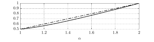
(a) Graph of $\frac{6\alpha^{3}+7\alpha^{2}-11\alpha+6}{9\alpha^{2}+17\alpha-10}$ and the optimal rate $\alpha/2$ (dashed) as a function of $\alpha$.

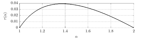
(b) Graph of $\tau(\alpha)$ given by (19).

Figure 5: The optimality gap for $\beta\in\left[{\alpha},{2}\right)$: Figure 5a shows the optimal and the obtained rate, and Figure 5b their difference $\tau(\alpha)$.

Let us also briefly discuss the two decay assumptions in the frequency domain on the shearlet generators in Theorem 13. Condition (i) says that $\psi$ is $(\delta,\gamma)$-feasible and can be interpreted as both a condition ensuring almost separable behavior and controlling the effective support of the shearlets in frequency domain as well as a moment condition along the $x_{1}$ axis, hence enforcing directional selectivity. Condition (ii), together with (i), is a weak version of a directional vanishing moment condition (see [13] for a precise definition), which is crucial for having fast decay of the shearlet coefficients when the corresponding shearlet intersects the discontinuity surface. We refer to the exposition [23] for a detailed explanation of the necessity of conditions (i) and (ii). Conditions (i) and (ii) are rather mild conditions on the generators; in particular, shearlets constructed by Theorem 10 and 11, with extra assumptions on the parameters $K$ and $L$, will indeed satisfy (i) and (ii) in Theorem 13. To compare with the optimality result for band-limited generators we wish to point out that conditions (i) and (ii) are obviously satisfied for band-limited generators.

Theorem 1.3 in [24] shows optimal sparse approximation of compactly supported shearlets in 2D. Theorem 13 is similar in spirit to Theorem 1.3 in [24], but for the three-dimensional setting. However, as opposed to the two-dimensional setting, anisotropic structures in three-dimensional data comprise of two morphological different types of structures, namely surfaces and curves. It would therefore be desirable to have a similar optimality result for our extended 3D image class ${\mathcal{E}}_{\alpha,L}^{\beta}(\mathbb{R}^{3})$ which also allows types of curve-like singularities. Yet, the pyramid-adapted shearlets introduced in Section 4.1 are plate-like and thus, a priori, not well-suited for capturing such one-dimensional singularities. However, these plate-like shearlet systems still deliver the nearly optimal error rate as the following result shows. The proof of the result is postponed to Section 10.

Theorem 14.

Let $\alpha\in\left({1},{2}\right]$, $c\in(\mathbb{R}_{+})^{2}$, and let $\phi,\psi,\tilde{\psi},\breve{\psi}\in L^{2}(\mathbb{R}^{3})$ be compactly supported. For each $\kappa\in[-1,1]$ and $x_{3}\in\mathbb{R}$, define $g^{0}_{\kappa,\,x_{3}}\in L^{2}(\mathbb{R}^{2})$ by

$$g^{0}_{\kappa,\,x_{3}}(x_{1},x_{2})=\psi(x_{1},x_{2},\kappa x_{2}+x_{3}),$$

and, for each $\kappa\in[-1,1]$ and $x_{2}\in\mathbb{R}$, define $g^{1}_{\kappa,\,x_{2}}\in L^{2}(\mathbb{R}^{2})$ by

$$g^{1}_{\kappa,\,x_{2}}(x_{1},x_{3})=\psi(x_{1},\kappa x_{3}+x_{2},x_{3}).$$

Suppose that, for all $\xi=(\xi_{1},\xi_{2},\xi_{3})\in\mathbb{R}^{3}$, $\kappa\in[-1,1]$, and $x_{2},x_{3}\in\mathbb{R}$, the function $\psi$ satisfies:

1. $|\hat{\psi}(\xi)|\leq C\cdot\min\{1,|\xi_{1}|^{\delta}\}\cdot\min\{1,|\xi_{1}|^{-\gamma}\}\cdot\min\{1,|\xi_{2}|^{-\gamma}\}\cdot\min\{1,|\xi_{3}|^{-\gamma}\}$,

2. $\left\lvert\bigl{(}\frac{\partial}{\partial\xi_{2}}\bigr{)}^{\ell}\hat{g}^{0}_{\kappa,\,x_{3}}(\xi_{1},\xi_{2})\right\rvert\leq|h(\xi_{1})|\cdot\left(1+\frac{|\xi_{2}|}{|\xi_{1}|}\right)^{-\gamma}\quad\text{for}\,\,\ell=0,1,$

3. $\left\lvert\bigl{(}\frac{\partial}{\partial\xi_{3}}\bigr{)}^{\ell}\hat{g}^{1}_{\kappa,\,x_{2}}(\xi_{1},\xi_{3})\right\rvert\leq|h(\xi_{1})|\cdot\left(1+\frac{|\xi_{3}|}{|\xi_{1}|}\right)^{-\gamma}\quad\text{for}\,\,\ell=0,1,$

where $\delta>8$, $\gamma\geq 4$, $h\in L^{1}(\mathbb{R})$, and $C$ a constant, and suppose that $\tilde{\psi}$ and $\breve{\psi}$ satisfy analogous conditions with the obvious change of coordinates. Further, suppose that the shearlet system $SH(\phi,\psi,\tilde{\psi},\breve{\psi};c,\alpha)$ forms a frame for $L^{2}(\mathbb{R}^{3})$.

Let $\beta\in\left[{\alpha},{2}\right]$. Then, for any $\nu>0$, $L>0$, and $\mu>0$, the shearlet frame $SH(\phi,\psi,\tilde{\psi},\breve{\psi};c,\alpha)$ provides nearly optimally sparse approximations of functions $f\in{\mathcal{E}}_{\alpha,L}^{\beta}(\mathbb{R}^{3})$ in the sense that

$$\left\lVert f-f_{N}\right\rVert_{L^{2}}^{2}\lesssim\left\{\begin{aligned} N^{-\alpha/2+\tau},&\qquad\text{if }\beta\in\left[{\alpha},{2}\right),\\ N^{-1}\,(\log{N})^{2},&\qquad\text{if }\beta=\alpha=2,\end{aligned}\right\}\text{ as $N\to\infty$,}$$

and

$$\left\lvert c^{*}_{n}\right\rvert\lesssim\left\{\begin{aligned} n^{-\frac{\alpha+2}{4}+\frac{\tau}{2}},&\qquad\text{if }\beta\in\left[{\alpha},{2}\right),\\ n^{-1}\,\log n,&\qquad\text{if }\beta=\alpha=2,\end{aligned}\right\}\text{ as $n\to\infty$,}$$

where $\tau=\tau(\alpha)$ is given by (19).

We remark that there exist numerous examples of $\psi,\tilde{\psi}$, and $\breve{\psi}$ satisfying the conditions (i) and (ii) in Theorem 13 and the conditions (i)-(iii) in Theorem 14. One large class of examples are separable generators $\psi,\tilde{\psi},\breve{\psi}\in L^{2}(\mathbb{R}^{3})$, i.e.,

$$\psi(x)=\eta(x_{1})\varphi(x_{2})\varphi(x_{3}),\quad\tilde{\psi}(x)=\varphi(x_{1})\eta(x_{2})\varphi(x_{3}),\quad\breve{\psi}(x)=\varphi(x_{1})\varphi(x_{2})\eta(x_{3}),$$

where $\eta,\varphi\in L^{2}(\mathbb{R})$ are compactly supported functions satisfying:

1. $|\hat{\eta}(\omega)|\leq C_{1}\cdot\min\{1,|\omega|^{\delta}\}\cdot\min\{1,|\omega|^{-\gamma}\}$,

2. $\left\lvert\bigl{(}\frac{\partial}{\partial\omega}\bigr{)}^{\ell}\hat{\varphi}(\omega)\right\rvert\leq C_{2}\cdot\min\{1,|\omega|^{-\gamma}\}\quad$ for $\ell=0,1$,

for $\omega\in\mathbb{R}$, where $\alpha>8$, $\gamma\geq 4$, and $C_{1},C_{2}$ are constants. Then it is straightforward to check that the shearlet $\psi$ satisfies the conditions (i)-(iii) in Theorem 14 and $\tilde{\psi},\breve{\psi}$ satisfy analogous conditions as required in Theorem 14. Thus, we have the following result.

Corollary 15.

Let $\alpha\in\left({1},{2}\right]$, $c\in(\mathbb{R}_{+})^{2}$, and let $\eta,\varphi\in L^{2}(\mathbb{R})$ be compactly supported functions satisfying:

1. $|\hat{\eta}(\omega)|\leq C_{1}\cdot\min\left\{{1,|\omega|^{\delta}}\right\}\cdot\min\left\{{1,|\omega|^{-\gamma}}\right\}$,

2. $\left\lvert\bigl{(}\frac{\partial}{\partial\omega}\bigr{)}^{\ell}\hat{\varphi}(\omega)\right\rvert\leq C_{2}\cdot\min\left\{{1,|\omega|^{-\gamma}}\right\}\quad$ for $\ell=0,1$,

for $\omega\in\mathbb{R}$, where $\delta>8$, $\gamma\geq 4$, and $C_{1}$ and $C_{2}$ are constants. Let $\phi\in L^{2}(\mathbb{R}^{3})$ be compactly supported, and let $\psi,\tilde{\psi},\breve{\psi}\in L^{2}(\mathbb{R}^{3})$ be defined by:

$$\psi(x)=\eta(x_{1})\varphi(x_{2})\varphi(x_{3}),\quad\tilde{\psi}(x)=\varphi(x_{1})\eta(x_{2})\varphi(x_{3}),\quad\breve{\psi}(x)=\varphi(x_{1})\varphi(x_{2})\eta(x_{3}).$$

Suppose that the shearlet system $SH(\phi,\psi,\tilde{\psi},\breve{\psi};c,\alpha)$ forms a frame for $L^{2}(\mathbb{R}^{3})$.

Let $\beta\in\left[{\alpha},{2}\right]$. Then, for any $\nu>0$, $L>0$, and $\mu>0$ , the shearlet frame $SH(\phi,\psi,\tilde{\psi},\breve{\psi};c,\alpha)$ provides nearly optimally sparse approximations of functions $f\in{\mathcal{E}}_{\alpha,L}^{\beta}(\mathbb{R}^{3})$ in the sense that

$$\left\lVert f-f_{N}\right\rVert_{L^{2}}^{2}\lesssim\left\{\begin{aligned} N^{-\alpha/2+\tau},&\qquad\text{if }\beta\in\left[{\alpha},{2}\right),\\ N^{-1}\,(\log{N})^{2},&\qquad\text{if }\beta=\alpha=2,\end{aligned}\right\}\text{ as $N\to\infty$,}$$

and

$$\left\lvert c^{*}_{n}\right\rvert\lesssim\left\{\begin{aligned} n^{-\frac{\alpha+2}{4}+\frac{\tau}{2}},&\qquad\text{if }\beta\in\left[{\alpha},{2}\right),\\ n^{-1}\,\log n,&\qquad\text{if }\beta=\alpha=2,\end{aligned}\right\}\text{ as $n\to\infty$,}$$

where $\tau=\tau(\alpha)$ is given by (19).

In the remaining sections of the paper we will prove Theorem 13 and Theorem 14.

6.2 General Organization of the Proofs of Theorems 13 and 14

Fix $\alpha\in\left({1},{2}\right]$ and $c\in(\mathbb{R}_{+})^{2}$, and take $B\in\mathit{STAR}^{\alpha}(\nu)$ and $f=f_{0}+\chi_{B}f_{1}\in{\mathcal{E}}_{\alpha}^{\beta}(\mathbb{R}^{3})$. Suppose $SH(\phi,\psi,\tilde{\psi},\breve{\psi};c,\alpha)$ satisfies the hypotheses of Theorem 13. Then by condition (i) the generators $\psi,\tilde{\psi}$ and $\breve{\psi}$ are absolute integrable in frequency domain hence continuous in time domain and therefore of finite max-norm $\left\lVert\cdot\right\rVert_{L^{\infty}}$. Let $A$ denote the lower frame bound of $SH(\phi,\psi,\tilde{\psi},\breve{\psi};c,\alpha)$.

Without loss of generality we can assume the scaling index $j$ to be sufficiently large. To see this note that $\mathop{\operator@font supp}\nolimits f\subset\left[{0},{1}\right]^{3}$ and all elements in the shearlet frame $SH(\phi,\psi,\tilde{\psi},\breve{\psi};c,\alpha)$ are compactly supported making the number of nonzero coefficients below a fixed scale $j_{0}$ finite. Since we are aiming for an asymptotic estimate, this finite number of coefficients can be neglected. This, in particular, means that we do not need to consider frame elements from the low pass system $\Phi(\phi;c)$. Furthermore, it suffices to consider shearlets $\Psi(\psi)=\{\psi_{j,k,m}\}$ associated with the pyramid ${\mathcal{P}}$ since the frame elements $\tilde{\psi}_{j,k,m}$ and $\breve{\psi}_{j,k,m}$ can be handled analogously.

To simplify notation, we denote our shearlet elements by $\psi_{\lambda}$, where $\lambda=(j,k,m)$ is indexing scale, shear, and position. We let $\Lambda_{j}$ be the indexing sets of shearlets in $\Psi(\psi)$ at scale $j$, i.e.,

$$\Psi(\psi)=\{\psi_{\lambda}:\lambda\in\Lambda_{j},j\geq 0\},$$

and collect these indices cross scales as

$$\Lambda=\bigcup_{j=0}^{\infty}\Lambda_{j}.$$

Our main concern will be to derive appropriate estimates for the shearlet coefficients $\left\{{\left\langle f,\psi_{\lambda}\right\rangle_{\!}}:{\lambda\in\Lambda}\right\}$ of $f$. Let $c(f)^{*}_{n}$ denote the $n$th largest shearlet coefficient $\left\langle f,\psi_{\lambda}\right\rangle_{\!}$ in absolute value. As mentioned in Section 3.3, to obtain the sought estimate on $\left\lVert f-f_{N}\right\rVert_{L^{2}}$ in (20), it suffices (by Lemma 2) to show that the $n$th largest shearlet coefficient $c(f)^{*}_{\,n}$ decays as specified by (21).

To derive the estimate in (21), we will study two separate cases. The first case for shearlet elements $\psi_{\lambda}$ that do not interact with the discontinuity surface, and the second case for those elements that do.

Case 1.

The compact support of the shearlet $\psi_{\lambda}$ does not intersect the boundary of the set $B$, i.e., $\left\lvert\mathop{\operator@font supp}\nolimits\psi_{\lambda}\cap\partial B\right\rvert=0$.

Case 2.

The compact support of the shearlet $\psi_{\lambda}$ does intersect the boundary of the set $B$, i.e., $\left\lvert\mathop{\operator@font supp}\nolimits\psi_{\lambda}\cap\partial B\right\rvert\neq 0$.

For Case 1 we will not be concerned with decay estimates of single coefficients $\left\langle f,\psi_{\lambda}\right\rangle_{\!}$, but with the decay of sums of coefficients over several scales and all shears and translations. The frame property of the shearlet system, the Sobolev smoothness of $f$ and a crude counting argument of the cardinal of the essential indices $\lambda$ will basically be enough to provide the needed approximation rate. We refer to Section 7 for the exact procedure.

For Case 2 we need to estimate each coefficient $\left\langle f,\psi_{\lambda}\right\rangle_{\!}$ individually and, in particular, how $\left\lvert\left\langle f,\psi_{\lambda}\right\rangle_{\!}\right\rvert$ decays with scale $j$ and shearing $k$. We assume, in the remainder of this section, that $f_{0}=0$ whereby $f=\chi_{B}f_{1}$. Depending on the orientation of the discontinuity surface, we will split Case 2 into several subcases. The estimates in each subcase will, however, follow the same principle: Let

$$M=\mathop{\operator@font supp}\nolimits\psi_{\lambda}\cap B.$$

Further, let $H$ be an affine hyperplane that intersects $M$ and thereby divides $M$ into two sets $M_{t}$ and $M_{l}$. We thereby have that

$$\left\langle f,\psi_{\lambda}\right\rangle_{\!}=\left\langle\chi_{M_{t}}f,\psi_{\lambda}\right\rangle_{\!}+\left\langle\chi_{M_{l}}f,\psi_{\lambda}\right\rangle_{\!}.$$

The hyperplane will be chosen in such way that $\operatorname{vol}{(M_{t})}$ is sufficiently small. In particular, $\operatorname{vol}{(M_{t})}$ should be small enough so that the following estimate

$$\left\lvert\left\langle\chi_{M_{t}}f,\psi_{\lambda}\right\rangle_{\!}\right\rvert\leq\left\lVert f\right\rVert_{L^{\infty}}\left\lVert\psi_{\lambda}\right\rVert_{L^{\infty}}\operatorname{vol}{(M_{t})}\leq\mu\,2^{j(\alpha+2)/4}\operatorname{vol}{(M_{t})}$$

does not violate (21). We call estimates of this form, where we have restricted the integration to a small part $M_{t}$ of $M$, truncated estimates (or the truncation term).

For the other term $\left\langle\chi_{M_{l}}f,\psi_{\lambda}\right\rangle_{\!}$ we will have to integrate over a possibly much large part $M_{l}$ of $M$. To handle this we will use that $\psi_{\lambda}$ only interacts with the discontinuity of $\chi_{M_{l}}f$ on a affine hyperplane inside $M$. This part of the estimate is called the linearized estimate (or the linearization term) since the discontinuity surface in $\left\langle\chi_{M_{l}}f,\psi_{\lambda}\right\rangle_{\!}$ has been reduced to a linear surface. In $\left\langle\chi_{M_{l}}f,\psi_{\lambda}\right\rangle_{\!}$ we are integrating over three variables, and we will as the inner integration always choose to integrate along lines parallel to the “singularity” hyperplane $H$. The important point here is that along all these line integrals, the function $f$ is $C^{\beta}$-smooth without discontinuities on the entire interval of integration. This is exactly the reason for removing the $M_{t}$-part from $M$. Using the Fourier slice theorem we will then turn the line integrations along $H$ in the spatial domain into two-dimensional plane integrations the frequency domain. The argumentation is as follows: Consider $g:\mathbb{R}^{3}\to\mathbb{C}$ compactly supported and continuous, and let $p:\mathbb{R}^{2}\to\mathbb{C}$ be a projection of $g$ onto, say, the $x_{2}$ axis, i.e., $p(x_{1},x_{3})=\int_{\mathbb{R}}g(x_{1},x_{2},x_{3})dx_{2}$. This immediately implies that $\hat{p}(\xi_{1},\xi_{3})=\hat{g}(\xi_{1},0,\xi_{3})$ which is a simplified version of the Fourier slice theorem. By an inverse Fourier transform, we then have

$$\int_{\mathbb{R}}g(x_{1},x_{2},x_{3})dx_{2}=p(x_{1},x_{3})=\int_{\mathbb{R}^{2}}\hat{g}(\xi_{1},0,\xi_{3})\mathrm{e}^{2\pi i\left\langle(x_{1},x_{3}),(\xi_{1},\xi_{3})\right\rangle_{\!}}\mathrm{d}\xi_{1}\mathrm{d}\xi_{3},$$ (22)

and hence

$$\int_{\mathbb{R}}\left\lvert g(x_{1},x_{2},x_{3})\right\rvert dx_{2}=\int_{\mathbb{R}^{2}}\left\lvert\hat{g}(\xi_{1},0,\xi_{3})\right\rvert\mathrm{d}\xi_{1}\mathrm{d}\xi_{3}.$$ (23)

The left-hand side of (23) corresponds to line integrations of $g$ parallel to the $x_{1}x_{3}$ plane. By applying shearing to the coordinates $x\in\mathbb{R}^{3}$, we can transform $H$ into a plane of the form $\left\{{x\in\mathbb{R}^{3}}:{x_{1}=C_{1},x_{3}=C_{2}}\right\}$, whereby we can apply (23) directly.

Finally, the decay assumptions on $\hat{\psi}$ in Theorem 13 are then used to derive decay estimates for $\left\lvert\left\langle f,\psi_{\lambda}\right\rangle_{\!}\right\rvert$. Careful counting arguments will enable us to arrive at the sought estimate in (21). We refer to Section 8 for a detailed description of Case 2.

With the sought estimates derived in Section 7 and 8, we then prove Theorem 13 in Section 9. The proof of Theorem 14 will follow the exact same organization and setup as Theorem 13. Since the proofs are almost identical, in the proof of Theorem 14, we will only focus on issues that need to be handled differently. The proof of Theorem 14 is presented in Section 10.

We end this section by fixing some notation used in the sequel. Since we are concerned with an asymptotic estimate, we will often simply use $C$ as a constant although it might differ for each estimate; sometimes we will simply drop the constant and use $\lesssim$ instead. We will also use the notation $r_{j}\sim s_{j}$ for $r_{j},s_{j}\in\mathbb{R}$, if $C_{1}\,r_{j}\leq s_{j}\leq C_{2}\,r_{j}$ with constants $C_{1}$ and $C_{2}$ independent on the scale $j$.

7 Analysis of shearlet coefficients away from the discontinuity surface

In this section we derive estimates for the decay rate of the shearlet coefficients $\left\langle f,\psi_{\lambda}\right\rangle_{\!}$ for Case 1 described in the previous section. Hence, we consider shearlets $\psi_{\lambda}$ whose support does not intersect the discontinuity surface $\partial B$. This means that $f$ is $C^{\beta}$-smooth on the entire support of $\psi_{\lambda}$, and we can therefore simply analyze shearlet coefficients $\left\langle f,\psi_{\lambda}\right\rangle_{\!}$ of functions $f\in C^{\beta}(\mathbb{R}^{3})$ with $\mathop{\operator@font supp}\nolimits f\subset\left[{0},{1}\right]^{3}$. The main result of this section, Proposition 18, shows that $\left\lVert f-f_{N}\right\rVert_{L^{2}}^{2}=O(N^{-2\beta/3+\varepsilon})$ as $N\to\infty$ for any $\varepsilon$, where $f_{N}$ is our $N$-term shearlet approximation. The result follows easily from Proposition 17 which is similar in spirit to Proposition 18, but for the case where $f\in H^{\beta}$. The proof builds on Lemma 16 which shows that the system $\Psi(\psi)$ forms a weighted Bessel-like sequence with strong weights such as $(2^{\alpha\beta j})_{j\geq 0}$ provided that the shearlet $\psi$ satisfies certain decay conditions. Lemma 16 is, in turn, proved by transferring Sobolev differentiability of the target function to decay properties in the Fourier domain and applying Lemma 12.

Lemma 16.

Let $g\in H^{\beta}(\mathbb{R}^{3})$ with $\mathop{\operator@font supp}\nolimits g\subset\left[{0},{1}\right]^{3}$. Suppose that $\psi\in L^{2}(\mathbb{R}^{3})$ is $(\delta,\gamma)$-feasible for $\delta>2\gamma+\beta$, $\gamma>3$. Then there exists a constant $B>0$ such that

$$\sum_{j=0}^{\infty}\sum_{\left\lvert k\right\rvert\leq\lceil 2^{j(\alpha-1)/2}\rceil}\sum_{m\in\mathbb{Z}^{3}}2^{\alpha\beta j}\left\lvert\left\langle g,\psi_{j,k,m}\right\rangle_{\!}\right\rvert^{2}\leq B\lVert\partial^{(\beta,0,0)}g\rVert_{L^{2}}^{2},$$

where $\partial^{(\beta,0,0)}g$ denotes the $\beta$-fractional partial derivative of $g=g(x_{1},x_{2},x_{3})$ with respect to $x_{1}$.

Proof.

Since $\psi\in L^{2}(\mathbb{R}^{3})$ is $(\delta,\gamma)$-feasible, we can choose $\varphi\in L^{2}(\mathbb{R}^{3})$ as

$$(2\pi i\xi_{1})^{\beta}\hat{\varphi}(\xi)=\hat{\psi}(\xi)\qquad\text{for }\xi\in\mathbb{R}^{3},$$

hence $\psi$ is the $\partial^{(\beta,0,0)}$-fractional derivative of $\varphi$. This definition is well-defined due to the decay assumptions on $\hat{\psi}$. By definition of the fractional derivative, it follows that

$$\bigl{\lvert}\bigl{\langle}\partial^{(\beta,0,0)}g,\varphi_{j,k,m}\bigr{\rangle}_{\!\!}\bigr{\rvert}^{2}=\left\lvert\left\langle(2\pi i\xi_{1})^{\beta}\hat{g}(\xi),\widehat{\varphi_{j,k,m}}\right\rangle_{\!}\right\rvert^{2}\\ =\bigl{\lvert}\bigl{\langle}g,\partial^{(\beta,0,0)}\varphi_{j,k,m}\bigr{\rangle}_{\!\!}\bigr{\rvert}^{2}=2^{\alpha\beta j}\left\lvert\left\langle g,\psi_{j,k,m}\right\rangle_{\!}\right\rvert^{2},$$

where we have used that $\partial^{(\beta,0,0)}f_{j,k,m}=(2^{j\alpha/2})^{\beta}(\partial^{(\beta,0,0)}f)_{j,k,m}$ for $f\in H^{\beta}(\mathbb{R}^{3})$. A straightforward computation shows that $\varphi$ satisfies the hypotheses of Lemma 12, and an application of Lemma 12 then yields

$$\sum_{j=0}^{\infty}\sum_{|k|\leq\lceil 2^{j(\alpha-1)/2}\rceil}\sum_{m\in\mathbb{Z}^{3}}2^{\alpha\beta j}|\langle g,\psi_{j,k,m}\rangle|^{2} =\sum_{j=0}^{\infty}\sum_{|k|\leq\lceil 2^{j(\alpha-1)/2}\rceil}\sum_{m\in\mathbb{Z}^{3}}\bigl{\lvert}\bigl{\langle}\partial^{(\beta,0,0)}g,\varphi_{j,k,m}\bigr{\rangle}_{\!\!}\bigr{\rvert}^{2}$$

$$\leq B\lVert\partial^{(\beta,0,0)}g\rVert_{L^{2}}^{2},$$

which completes the proof. ∎

We are now ready to prove the following result.

Proposition 17.

Let $g\in H^{\beta}(\mathbb{R}^{3})$ with $\mathop{\operator@font supp}\nolimits g\subset\left[{0},{1}\right]^{3}$. Suppose that $\psi\in L^{2}(\mathbb{R}^{3})$ is compactly supported and $(\delta,\gamma)$-feasible for $\delta>2\gamma+\beta$ and $\gamma>3$. Then

$$\sum_{n>N}\left\lvert c(g)^{*}_{n}\right\rvert^{2}\lesssim N^{-2\beta/3}\qquad\text{as}\quad N\to\infty,$$

where $c(g)^{*}_{n}$ is the $n$th largest coefficient $\left\langle g,\psi_{\lambda}\right\rangle_{\!}$ in modulus for $\psi_{\lambda}\in\Psi(\psi)$.

Proof.

Set

$$\tilde{\Lambda}_{j}=\{\lambda\in\Lambda_{j}:\mathop{\operator@font supp}\nolimits\psi_{\lambda}\cap\mathop{\operator@font supp}\nolimits g\neq\emptyset\},\quad j>0,$$

i.e., $\tilde{\Lambda}_{j}$ is the set of indices in $\Lambda_{j}$ associated with shearlets whose support intersects the support of $g$. Then, for each scale $J>0$, we have

$$N_{J}=\Big{|}\bigcup_{j=0}^{J-1}\tilde{\Lambda}_{j}\Big{|}\sim\sum_{j=0}^{J-1}(2^{j(\alpha-1)/2})^{2}\,2^{j\alpha/2}\,2^{j/2}\,2^{j/2}=2^{(3/2)\alpha J},$$ (24)

where the term $(2^{j(\alpha-1)/2})^{2}$ is due to the number of shearing $\left\lvert k\right\rvert=\left\lvert(k_{1},k_{2})\right\rvert\in 2^{j(\alpha-1)/2}$ at scale $j$ and the term $2^{j\alpha/2}\,2^{j/2}\,2^{j/2}$ is due to the number of translation for which $g$ and $\psi_{\lambda}$ interact; recall that $\psi_{\lambda}$ has support in a set of measure $2^{-j\alpha/2}\cdot 2^{-j/2}\cdot 2^{-j/2}$.

We observe that there exists some $C>0$ such that

$$\sum_{j_{0}=1}^{\infty}2^{\alpha\beta j_{0}}\sum_{n>N_{j_{0}}}|c(g)^{*}_{n}|^{2} \leq C\cdot\sum_{j_{0}=1}^{\infty}\sum_{j=j_{0}}^{\infty}\sum_{k,m}2^{\alpha\beta j_{0}}|\langle g,\psi_{j,k,m}\rangle|^{2}$$

$$=C\cdot\sum_{j=1}^{\infty}\sum_{k,m}|\langle g,\psi_{j,k,m}\rangle|^{2}\biggl{(}\sum_{j_{0}=1}^{j}2^{\alpha\beta j_{0}}\biggr{)}.$$

By Lemma 16, this yields

$$\sum_{j_{0}=1}^{\infty}2^{\alpha\beta j_{0}}\sum_{n>N_{j_{0}}}|c(g)^{*}_{n}|^{2}\leq C\cdot\sum_{j=1}^{\infty}\sum_{k,m}2^{\alpha\beta j}|\langle g,\psi_{j,k,m}\rangle|^{2}<\infty,$$

and thus, by (24), that

$$\sum_{n>N_{j_{0}}}|c(g)^{*}_{n}|^{2}\leq C\cdot 2^{-\alpha\beta j_{0}}=C\cdot(2^{(3/2)\alpha j_{0}})^{-2\beta/3}\leq C\cdot N_{j_{0}}^{\,-2\beta/3}.$$

Finally, let $N>0$. Then there exists a positive integer $j_{0}>0$ such that

$$N\sim N_{j_{0}}\sim 2^{(3/2)\alpha j_{0}},$$

which completes the proof. ∎

We can get rid of the Sobolev space requirement in Proposition 17 if we accept a slightly worse decay rate.

Proposition 18.

Let $f\in C^{\beta}(\mathbb{R}^{3})$ with $\mathop{\operator@font supp}\nolimits g\subset\left[{0},{1}\right]^{3}$. Suppose that $\psi\in L^{2}(\mathbb{R}^{3})$ is compactly supported and $(\delta,\gamma)$-feasible for $\delta>2\gamma+\beta$ and $\gamma>3$. Then

$$\sum_{n>N}\left\lvert c(g)^{*}_{n}\right\rvert^{2}\lesssim N^{-2\beta/3+\varepsilon}\qquad\text{as}\quad N\to\infty,$$

for any $\varepsilon>0$.

Proof.

By the intrinsic characterization of fractional order Sobolev spaces [1], we see that $C^{\beta}_{0}(\mathbb{R}^{3})\subset H^{\beta-\varepsilon}_{0}(\mathbb{R}^{3})$ for any $\varepsilon>0$. The result now follows from Proposition 17. ∎

8 Analysis of shearlet coefficients associated with the discontinuity surface

We now turn our attention to Case 2. Here we have to estimate those shearlet coefficients whose support intersects the discontinuity surface. For any scale $j\geq 0$ and any grid point $p\in\mathbb{Z}^{3}$, we let ${\mathcal{Q}}_{j,p}$ denote the dyadic cube defined by

$${\mathcal{Q}}_{j,p}=[-2^{-j/2},2^{-j/2}]^{3}+2^{-j/2}2p.$$

We let ${\mathcal{Q}}_{j}$ be the collection of those dyadic cubes ${\mathcal{Q}}_{j,p}$ at scale $j$ whose interior $\operatorname{int}({\mathcal{Q}}_{j,p})$ intersects $\partial B$, i.e.,

$${\mathcal{Q}}_{j}=\{{\mathcal{Q}}_{j,p}:\operatorname{int}({\mathcal{Q}}_{j,p})\cap\partial B\neq\emptyset,p\in\mathbb{Z}^{3}\}.$$

Of interest to us are not only the dyadic cubes, but also the shearlet indices associated with shearlets intersecting the discontinuity surface inside some ${\mathcal{Q}}_{j,p}\in{\mathcal{Q}}_{j}$, i.e., for $j\geq 0$ and $p\in\mathbb{Z}^{3}$ with ${\mathcal{Q}}_{j,p}\in{\mathcal{Q}}_{j}$, we will consider the index set

$${\Lambda_{j,p}}=\{\lambda\in\Lambda_{j}:\operatorname{int}(\mathop{\operator@font supp}\nolimits\psi_{\lambda})\cap\operatorname{int}({\mathcal{Q}}_{j,p})\cap\partial B\neq\emptyset\}.$$

Further, for $j\geq 0$, $p\in\mathbb{Z}^{3}$, and $0<\varepsilon<1$, we define $\Lambda_{j,p}(\varepsilon)$ to be the index set of shearlets $\psi_{\lambda}$, $\lambda\in{\Lambda_{j,p}}$, such that the magnitude of the corresponding shearlet coefficient $\langle f,\psi_{\lambda}\rangle$ is larger than $\varepsilon$ and the support of $\psi_{\lambda}$ intersects ${\mathcal{Q}}_{j,p}$ at the $j$th scale, i.e.,

$${\Lambda_{j,p}(\varepsilon)}=\{\lambda\in{\Lambda_{j,p}}:|\langle f,\psi_{\lambda}\rangle|>\varepsilon\}.$$

The collection of such shearlet indices across scales and translates will be denoted by $\Lambda(\varepsilon)$, i.e.,

$$\Lambda(\varepsilon)=\bigcup_{j,p}\Lambda_{j,p}(\varepsilon).$$

As mentioned in Section 6.2, we may assume that $j$ is sufficiently large. Suppose ${\mathcal{Q}}_{j,p}\in{\mathcal{Q}}_{j}$ for some given scale $j\geq 0$ and position $p\in\mathbb{Z}^{3}$. Then the set

$${\mathcal{S}}_{j,p}=\bigcup_{\lambda\in\Lambda_{j,p}}\mathop{\operator@font supp}\nolimits\psi_{\lambda}$$

is contained in a cube of size $C\cdot 2^{-j/2}$ by $C\cdot 2^{-j/2}$ by $C\cdot 2^{-j/2}$ and is, thereby, asymptotically of the same size as ${\mathcal{Q}}_{j,p}$.

We now restrict ourselves to considering $B\in\mathit{STAR}^{\alpha}(\nu)$; the piecewise case $B\in\mathit{STAR}^{\alpha}(\nu,L)$ will be dealt with in Section 10. By smoothness assumption on the discontinuity surface $\partial B$, the discontinuity surface can locally be parametrized by either $(x_{1},x_{2},E(x_{1},x_{2}))$, $(x_{1},E(x_{1},x_{3}),x_{3})$, or $(E(x_{2},x_{3}),x_{2},x_{3})$ with $E\in C^{\alpha}$ in the interior of ${\mathcal{S}}_{j,p}$ for sufficiently large $j$. In other words, the part of the discontinuity surface $\partial B$ contained in ${\mathcal{S}}_{j,p}$ can be described as the graph $x_{3}=E(x_{1},x_{2})$, $x_{2}=E(x_{1},x_{3})$, or $x_{1}=E(x_{2},x_{3})$ of a $C^{\alpha}$ function.

Thus, we are facing the following two cases:

Case 2a.

The discontinuity surface $\partial B$ can be parametrized by $(E(x_{2},x_{3}),x_{2},x_{3})$ with $E\in C^{\alpha}$ in the interior of ${\mathcal{S}}_{j,p}$ such that, for any $\lambda\in\Lambda_{j,p}$, we have

$$|\partial^{(1,0)}E(\hat{x}_{2},\hat{x}_{3})|<+\infty\quad\text{and}\quad|\partial^{(0,1)}E(\hat{x}_{2},\hat{x}_{3})|<+\infty,$$

for all $\hat{x}=(\hat{x}_{1},\hat{x}_{2},\hat{x}_{3})\in\operatorname{int}({\mathcal{Q}}_{j,p})\cap\operatorname{int}(\mathop{\operator@font supp}\nolimits\psi_{\lambda})\cap\partial B$.

Case 2b.

The discontinuity surface $\partial B$ can be parametrized by $(x_{1},x_{2},E(x_{1},x_{2}))$ or $(x_{1},E(x_{1},x_{3}),x_{3})$ with $E\in C^{\alpha}$ in the interior of ${\mathcal{S}}_{j,p}$ such that, for any $\lambda\in\Lambda_{j,p}$, there exists some $\hat{x}=(\hat{x}_{1},\hat{x}_{2},\hat{x}_{3})\in\operatorname{int}({\mathcal{Q}}_{j,p})\cap\operatorname{int}(\mathop{\operator@font supp}\nolimits\psi_{\lambda})\cap\partial B$ satisfying

$$\partial^{(1,0)}E(\hat{x}_{1},\hat{x}_{2})=0\quad\text{or}\quad\partial^{(1,0)}E(\hat{x}_{1},\hat{x}_{3})=0.$$

8.1 Hyperplane discontinuity

As described in Section 6.2, the linearized estimates of the shearlet coefficients will be one of the key estimates in proving Theorem 13. Linearized estimates are used in the slightly simplified situation, where the discontinuity surface is linear. Since such an estimate is interesting in it own right, we state and prove a linearized estimation result below. Moreover, we will use the methods developed in the proof repeatedly in the remaining sections of the paper. In the proof, we will see that the shearing operation is indeed very effective when analyzing hyperplane singularities.

Theorem 19.

Let $\psi\in L^{2}(\mathbb{R}^{3})$ be compactly supported, and assume that $\psi$ satisfies conditions (i) and (ii) of Theorem 13. Further, let $\lambda\in\Lambda_{j,p}$ for $j\geq 0$ and $p\in\mathbb{Z}^{3}$. Suppose that $f\in{\mathcal{E}}_{\alpha}^{\beta}(\mathbb{R}^{3})$ for $1<\alpha\leq\beta\leq 2$ and that $\partial B$ is linear on the support of $\psi_{\lambda}$ in the sense that

$$\mathop{\operator@font supp}\nolimits\psi_{\lambda}\cap\partial B\subset H$$

for some affine hyperplane $H$ of $\mathbb{R}^{3}$. Then,

1. if $H$ has normal vector $(-1,s_{1},s_{2})$ with $s_{1}\leq 3$ and $s_{2}\leq 3$,

   $$|\langle f,\psi_{\lambda}\rangle|\leq C\cdot\min_{i=1,2}\left\{\frac{2^{-j(\alpha/4+1/2)}}{|k_{i}+2^{j(\alpha-1)/2}s_{i}|^{3}}\right\},$$ (25)

   for some constant $C>0$.

2. if $H$ has normal vector $(-1,s_{1},s_{2})$ with $s_{1}\geq 3/2$ or $s_{2}\geq 3/2$,

   $$|\langle f,\psi_{\lambda}\rangle|\leq C\cdot 2^{-j(\alpha/4+1/2+\alpha\beta/2)}$$ (26)

   for some constant $C>0$.

3. if $H$ has normal vector $(0,s_{1},s_{2})$ with $s_{1},s_{2}\in\mathbb{R}$, then (26) holds.

Proof.

Let us fix $(j,k,m)\in\Lambda_{j,p}$ and $f\in{\mathcal{E}}_{\alpha}^{\beta}(\mathbb{R}^{3})$. We can without loss of generality assume that $f$ is only nonzero on $B$. We first consider the cases (i) and (ii). The hyperplane can be written as

$$H=\left\{{x\in\mathbb{R}^{3}}:{\left\langle x-x_{0},(-1,s_{1},s_{2})\right\rangle_{\!}=0}\right\}$$

for some $x_{0}\in\mathbb{R}^{3}$. We shear the hyperplane by $S_{-s}$ for $s=(s_{1},s_{2})$ and obtain

$$S_{-s}H =\left\{{x\in\mathbb{R}^{3}}:{\left\langle S_{s}x-x_{0},(-1,s_{1},s_{2})\right\rangle_{\!}=0}\right\}$$

$$=\left\{{x\in\mathbb{R}^{3}}:{\left\langle x-S_{-s}x_{0},(S_{s})^{T}(-1,s_{1},s_{2})\right\rangle_{\!}=0}\right\}$$

$$=\left\{{x\in\mathbb{R}^{3}}:{\left\langle x-S_{-s}x_{0},(-1,0,0)\right\rangle_{\!}=0}\right\}$$

$$=\left\{{x=(x_{1},x_{2},x_{3})\in\mathbb{R}^{3}}:{x_{1}=\hat{x}_{1}}\right\},\quad\text{where $\hat{x}=S_{-s}x_{0}$,}$$

which is a hyperplane parallel to the $x_{2}x_{3}$ plane. Here the power of shearlets comes into play since it will allow us to only consider hyperplane singularities parallel to the $x_{2}x_{3}$ plane. Of course, this requires that we also modify the shear parameter of the shearlet, that is, we will consider the right hand side of

$${\left\langle f,\psi_{j,k,m}\right\rangle_{\!}}={\langle f(S_{s}\cdot),\psi_{j,\hat{k},m}\rangle}$$

with the new shear parameter $\hat{k}$ defined by $\hat{k}_{1}=k_{1}+2^{j(\alpha-1)/2}s_{1}$ and $\hat{k}_{2}=k_{2}+2^{j(\alpha-1)/2}s_{2}$. The integrand in $\langle f(S_{s}\cdot),\psi_{j,\hat{k},m}\rangle$ has the singularity plane exactly located on $x_{1}=\hat{x}_{1}$, i.e., on $S_{-s}H$.

To simplify the expression for the integration bounds, we will fix a new origin on $S_{-s}H$, that is, on $x_{1}=\hat{x}_{1}$; the $x_{2}$ and $x_{3}$ coordinate of the new origin will be fixed in the next paragraph. Since $f$ is assumed to be only nonzero on $B$, the function $f$ will be equal to zero on one side of $S_{-s}H$, say, $x_{1}<\hat{x}_{1}$. It therefore suffices to estimate

$${\langle f_{0}(S_{s}\cdot)\chi_{\Omega},\psi_{j,\hat{k},m}\rangle}$$

for $f_{0}\in C^{\beta}(\mathbb{R}^{3})$ and $\Omega=\mathbb{R}_{+}\times\mathbb{R}^{2}$. We first consider the case $\lvert\hat{k}_{1}\rvert\leq\lvert\hat{k}_{2}\rvert$. We further assume that $\hat{k}_{1}<0$ and $\hat{k}_{2}<0$. The other cases can be handled similarly.

Since $\psi$ is compactly supported, there exists some $L>0$ such that $\mathop{\operator@font supp}\nolimits{\psi}\subset\left[{-L},{L}\right]^{3}$. By a rescaling argument, we can assume $L=1$. Let

$${\mathcal{P}}_{j,k}:=\left\{{x\in\mathbb{R}^{3}}:{\lvert 2^{j\alpha/2}x_{1}+2^{j/2}\hat{k}_{1}x_{2}+2^{j/2}\hat{k}_{2}x_{3}\rvert\leq 1,\left\lvert x_{2}\right\rvert,\left\lvert x_{3}\right\rvert\leq 2^{-j/2}}\right\},$$ (27)

With this notation, we have $\mathop{\operator@font supp}\nolimits\psi_{j,k,0}\subset{\mathcal{P}}_{j,k}$. We say that the shearlet normal direction of the shearlet box ${\mathcal{P}}_{j,0}$ is $(1,0,0)$, thus the shearlet normal of a sheared element $\psi_{j,k,m}$ associated with ${\mathcal{P}}_{j,k}$ is $(1,k_{1}/2^{j(\alpha-1)/2},k_{2}/2^{j(\alpha-1)/2})$. Now, we fix our origin so that, relative to this new origin, it holds that

$$\mathop{\operator@font supp}\nolimits(\psi_{j,\hat{k},m})\subset{\mathcal{P}}_{j,\hat{k}}+(2^{-j\alpha/2},0,0)=:\tilde{{\mathcal{P}}}_{j,\hat{k}}.$$

Then one face of $\tilde{{\mathcal{P}}}_{j,\hat{k}}$ intersects the origin.

For a fixed $\left\lvert\hat{x}_{3}\right\rvert\leq 2^{-j/2}$, we consider the cross section of the parallelepiped $\tilde{{\mathcal{P}}}_{j,\hat{k}}$ on the hyperplane $x_{3}=\hat{x}_{3}$. This cross section will be a parallelogram with sides $x_{2}=\pm 2^{-j/2}$,

$$2^{j\alpha/2}x_{1}+2^{j/2}\hat{k}_{1}x_{2}+2^{j/2}\hat{k}_{2}x_{3}=0,\;\text{ and }\;2^{j\alpha/2}x_{1}+2^{j/2}\hat{k}_{1}x_{2}+2^{j/2}\hat{k}_{2}x_{3}=2.$$

As it is only a matter of scaling we replace the right hand side of the last equation with $1$ for simplicity. Solving the two last equalities for $x_{2}$ gives the following lines on the hyperplane $x_{3}=\hat{x}_{3}$:

$$L_{1}:\;x_{2}=-\frac{2^{j(\alpha-1)/2}}{\hat{k}_{1}}x_{1}-\frac{\hat{k}_{2}}{\hat{k}_{1}}x_{3},\;\;\text{ and }\;\;L_{2}:\;x_{2}=-\frac{2^{j(\alpha-1)/2}}{\hat{k}_{1}}x_{1}-\frac{\hat{k}_{2}}{\hat{k}_{1}}x_{3}+\frac{2^{-j/2}}{\hat{k}_{1}}.$$

We therefore have

$$\left\lvert\left\langle f_{0}(S_{s}\cdot)\chi_{\Omega},\psi_{j,\hat{k},m}\right\rangle_{\!}\right\rvert\lesssim\left\lvert\int_{-2^{-j/2}}^{2^{-j/2}}\int_{0}^{K_{1}}\int_{L_{2}}^{L_{1}}f_{0}(S_{s}x)\psi_{j,\hat{k},m}(x)\,\mathrm{d}x_{2}\mathrm{d}x_{1}\mathrm{d}x_{3}\right\rvert,$$ (28)

where the upper integration bound for $x_{1}$ is $K_{1}=2^{-j(\alpha/2)}-2^{-j\alpha/2}\hat{k}_{1}-2^{j(\alpha-1)/2}\hat{k}_{2}x_{3}$ which follows from solving $L_{2}$ for $x_{1}$ and using that $\left\lvert x_{2}\right\rvert\leq 2^{-j/2}$. We remark that the inner integration over $x_{2}$ is along lines parallel to the singularity plane $\partial\Omega=\{0\}\times\mathbb{R}^{2}$; as mentioned, this allows us to better handle the singularity and will be used several times throughout this paper.

For a fixed $\left\lvert x_{3}\right\rvert\leq 2^{-j/2}$, we consider the one-dimensional Taylor expansion for $f_{0}(S_{s}\cdot)$ at each point $x=(x_{1},x_{2},x_{3})\in L_{2}$ in the $x_{2}$-direction:

$$f_{0}(S_{s}x) =a(x_{1},x_{3})+b(x_{1},x_{3})\left(x_{2}+\frac{2^{j(\alpha-1)/2}}{\hat{k}_{1}}\ x_{1}+\frac{\hat{k}_{2}}{\hat{k}_{1}}x_{3}-\frac{2^{-j/2}}{\hat{k}_{1}}\right)$$

$$\phantom{=}+c(x_{1},x_{2},x_{3})\left(x_{2}+\frac{2^{j(\alpha-1)/2}}{\hat{k}_{1}}\ x_{1}+\frac{\hat{k}_{2}}{\hat{k}_{1}}x_{3}-\frac{2^{-j/2}}{\hat{k}_{1}}\right)^{\beta},$$

where $a(x_{1},x_{3}),b(x_{1},x_{3})$ and $c(x_{1},x_{2},x_{3})$ are all bounded in absolute value by $C(1+\left\lvert s_{1}\right\rvert)^{\beta}$. Using this Taylor expansion in (28) yields

$$\left\lvert\left\langle f_{0}(S_{s}\cdot)\chi_{\Omega},\psi_{j,\hat{k},m}\right\rangle_{\!}\right\rvert\lesssim(1+\left\lvert s_{1}\right\rvert)^{\beta}\left\lvert\int_{-2^{-j/2}}^{2^{-j/2}}\int_{0}^{K_{1}}\sum_{l=1}^{3}I_{l}(x_{1},x_{3})\,\mathrm{d}x_{1}\mathrm{d}x_{3}\right\rvert,$$ (29)

where

$$I_{1}(x_{1},x_{3}) =\left\lvert\int_{L_{1}}^{L_{2}}\psi_{j,\hat{k},m}(x)\mathrm{d}x_{2}\right\rvert,$$

$$I_{2}(x_{1},x_{3}) =\left\lvert\int_{L_{1}}^{L_{2}}(x_{2}+K_{2})\,\psi_{j,\hat{k},m}(x)\mathrm{d}x_{2}\right\rvert,$$

$$I_{3}(x_{1},x_{3}) =\left\lvert\int_{0}^{-2^{-j/2}/\hat{k}_{1}}(x_{2})^{\beta}\,\psi_{j,\hat{k},m}(x_{1},x_{2}-K_{2},x_{3})\mathrm{d}x_{2}\right\rvert,$$

and

$$K_{2}=\frac{2^{j(\alpha-1)/2}}{\hat{k}_{1}}\ x_{1}+\frac{\hat{k}_{2}}{\hat{k}_{1}}x_{3}-\frac{2^{-j/2}}{\hat{k}_{1}}.$$

We next estimate each of the integrals $I_{1}$, $I_{2}$, and $I_{3}$ separately. We start with estimating $I_{1}(x_{1},x_{3})$. The Fourier Slice Theorem (22) yields directly that

$$I_{1}(x_{1},x_{3})=\Bigl{\lvert}\int_{\mathbb{R}}\psi_{j,\hat{k},m}(x)\mathrm{d}x_{2}\Bigr{\rvert}=\Bigl{\lvert}\int_{\mathbb{R}^{2}}\hat{\psi}_{j,\hat{k},m}(\xi_{1},0,\xi_{3})\,\mathrm{e}^{2\pi i\left\langle(x_{1},x_{3}),(\xi_{1},\xi_{3})\right\rangle_{\!}}\mathrm{d}\xi_{1}\mathrm{d}\xi_{3}\Bigr{\rvert}.$$

By assumptions (i) and (ii) from Theorem 13, we have, for all $\xi=(\xi_{1},\xi_{2},\xi_{3})\in\mathbb{R}^{3}$,

$$\bigl{\lvert}\hat{\psi}_{j,\hat{k},m}(\xi)\bigr{\rvert}\lesssim 2^{-j\frac{2+\alpha}{4}}\bigl{\lvert}h(2^{-j\alpha/2}\xi_{1})\bigr{\rvert}\left(1+\Bigl{\lvert}\tfrac{2^{-j/2}\xi_{2}}{2^{-j\alpha/2}\xi_{1}}+\hat{k}_{1}\Bigr{\rvert}\right)^{-\gamma}\left(1+\Bigl{\lvert}\tfrac{2^{-j/2}\xi_{3}}{2^{-j\alpha/2}\xi_{1}}+\hat{k}_{2}\Bigr{\rvert}\right)^{-\gamma}$$

for some $h\in L^{1}(\mathbb{R})$. Hence, we can continue our estimate of $I_{1}$:

$$I_{1}(x_{1},x_{3})\lesssim\int_{\mathbb{R}^{2}}2^{-j\frac{2+\alpha}{4}}\bigl{\lvert}h(2^{-j\alpha/2}\xi_{1})\bigr{\rvert}(1+\lvert\hat{k}_{1}\rvert)^{-\gamma}\left(1+\Bigl{\lvert}\tfrac{2^{-j/2}\xi_{3}}{2^{-j\alpha/2}\xi_{1}}+\hat{k}_{2}\Bigr{\rvert}\right)^{-\gamma}\mathrm{d}\xi_{1}\mathrm{d}\xi_{3},$$

and further, by a change of variables,

$$I_{1}(x_{1},x_{3}) \lesssim\int_{\mathbb{R}^{2}}2^{j\alpha/4}\left\lvert h(\xi_{1})\right\rvert(1+\lvert\hat{k}_{1}\rvert)^{-\gamma}\left(1+\left\lvert\frac{\xi_{3}}{\xi_{1}}+\hat{k}_{2}\right\rvert\right)^{-\gamma}\mathrm{d}\xi_{1}\mathrm{d}\xi_{3}$$

$$\lesssim 2^{j\alpha/4}(1+\lvert\hat{k}_{1}\rvert)^{-\gamma},$$

since $h\in L^{1}(\mathbb{R})$ and $(1+\lvert\xi_{3}/\xi_{1}+\hat{k}_{2}\rvert)^{-\gamma}=O(1)$ as $\left\lvert\xi_{1}\right\rvert\to\infty$ for fixed $\xi_{3}$.

We estimate $I_{2}(x_{1},x_{3})$ by

$$I_{2}(x_{1},x_{3})\leq\left\lvert\int_{\mathbb{R}}x_{2}\,\psi_{j,\hat{k},m}(x)\mathrm{d}x_{2}\right\rvert+\left\lvert K_{2}\right\rvert\left\lvert\int_{\mathbb{R}}\psi_{j,\hat{k},m}(x)\mathrm{d}x_{2}\right\rvert=:S_{1}+S_{2}$$

Applying the Fourier Slice Theorem again and then utilizing the decay assumptions on $\hat{\psi}$ yields

$$S_{1} =\left\lvert\int_{\mathbb{R}}x_{2}\psi_{j,\hat{k},m}(x)\mathrm{d}x_{2}\right\rvert$$

$$\leq\left\lvert\int_{\mathbb{R}^{2}}\left(\frac{\partial}{\partial\xi_{2}}\hat{\psi}_{j,\hat{k},m}\right)(\xi_{1},0,\xi_{3})\,\mathrm{e}^{2\pi i\left\langle(x_{1},x_{3}),(\xi_{1},\xi_{3})\right\rangle_{\!}}\mathrm{d}\xi_{1}\mathrm{d}\xi_{3}\right\rvert\lesssim\frac{2^{j(\alpha/4-1/2)}}{(1+\lvert\hat{k}_{1}\rvert)^{\beta+1}}.$$

Since $\left\lvert x_{1}\right\rvert\leq-\hat{k}_{1}/2^{j}$ and $\left\lvert\xi_{3}\right\rvert\leq 2^{-j/2}$, we have that

$$K_{2}\leq\left\lvert\frac{2^{j(\alpha-1)/2}}{\hat{k}_{1}}\ \frac{\hat{k}_{1}}{2^{j}}+2^{-j/2}-\frac{2^{-j/2}}{\hat{k}_{1}}\right\rvert,$$

The following estimate of $S_{2}$ then follows directly from the estimate of $I_{1}$:

$$S_{2}\lesssim\left\lvert K_{2}\right\rvert 2^{j\alpha/4}\,(1+\lvert\hat{k}_{1}\rvert)^{-\gamma}\lesssim 2^{j(\alpha/4-1/2)}(1+\lvert\hat{k}_{1}\rvert)^{-\gamma}.$$

From the two last estimate, we conclude that $I_{2}(x_{1},x_{3}s)\lesssim\frac{2^{j(\alpha/4-1/2)}}{(1+\lvert\hat{k}_{1}\rvert)^{\beta+1}}$.

Finally, we estimate $I_{3}(x_{1},x_{3})$ by

$$I_{3}(x_{1},x_{3}) \leq\left\lvert\int_{0}^{-2^{-j/2}/\hat{k}_{1}}(x_{2})^{\beta}\,\lVert\psi_{j,\hat{k},m}\rVert_{L^{\infty}}\,\mathrm{d}x_{2}\right\rvert$$

$$\lesssim 2^{j(\alpha/4+1/2)}\left\lvert\int_{0}^{-2^{-j/2}/\hat{k}_{1}}(x_{2})^{\beta}\,\mathrm{d}x_{2}\right\rvert=\frac{2^{j(\alpha/4-\beta/2)}}{\lvert\hat{k}_{1}\rvert^{\beta+1}}.$$

Having estimated $I_{1}$, $I_{2}$ and $I_{3}$, we continue with (29) and obtain

$$\left\lvert\left\langle f_{0}(S_{s}\cdot)\chi_{\Omega},\psi_{j,\hat{k},m}\right\rangle_{\!}\right\rvert\lesssim(1+\left\lvert s_{1}\right\rvert)^{\beta}\left(\frac{2^{-j(\alpha/4+1/2)}}{(1+\lvert\hat{k}_{1}\rvert)^{\gamma-1}}+\frac{2^{-j(\alpha/4+1/2+\beta/2)}}{\lvert\hat{k}_{1}\rvert^{\beta}}\right).$$

By performing a similar analysis for the case $\lvert\hat{k}_{2}\rvert\leq\lvert\hat{k}_{1}\rvert$, we arrive at

$$\bigl{\lvert}\left\langle f_{0}(S_{s}\cdot)\chi_{\Omega},\psi_{j,\hat{k},m}\right\rangle_{\!}\bigr{\rvert}\lesssim\min_{i=1,2}\left\{(1+\left\lvert s_{i}\right\rvert)^{\beta}\left(\frac{2^{-j(\alpha/4+1/2)}}{(1+\lvert\hat{k}_{i}\rvert)^{\gamma-1}}+\frac{2^{-j(\alpha/4+1/2+\beta/2)}}{\lvert\hat{k}_{i}\rvert^{\beta}}\right)\right\}$$ (30)

Suppose that $s_{1}\leq 3$ and $s_{2}\leq 3$. Then (30) reduces to

$$\left\lvert\left\langle f,\psi_{j,k,m}\right\rangle_{\!}\right\rvert \lesssim\min_{i=1,2}\left\{\frac{2^{-j(\alpha/4+1/2)}}{(1+\lvert\hat{k}_{i}\rvert)^{\gamma-1}}+\frac{2^{-j(\alpha/4+\beta/2+1/2)}}{\lvert\hat{k}_{i}\rvert^{\beta}}\right\}$$

$$\lesssim\min_{i=1,2}\left\{\frac{2^{-j(\alpha/4+1/2)}}{|k_{i}+2^{j(\alpha-1)/2}s_{i}|^{3}}\right\},$$

since $\gamma\geq 4$ and $\beta\geq\alpha$. On the other hand, if $s_{1}\geq 3/2$ or $s_{1}\geq 3/2$, then

$$\bigl{\lvert}\left\langle f,\psi_{j,k,m}\right\rangle_{\!}\bigr{\rvert}\lesssim 2^{-j(\alpha/2+1/4)\alpha}.$$

To see this, note that

$$\min_{i=1,2}\left\{(1+\left\lvert s_{i}\right\rvert)^{\beta}\frac{2^{-j(\alpha/4+\beta/2+1/2)}}{(1+\lvert\hat{k}_{i}\rvert)^{\beta}}\right\}=\min_{i=1,2}\left\{\tfrac{(1+\left\lvert s_{i}\right\rvert)^{\beta}}{\left\lvert s_{i}\right\rvert^{\beta}}\frac{2^{-j(\alpha/4+\beta/2+1/2)}}{(\lvert(1+k_{i})/s_{i}+2^{j(\alpha-1)/2}\rvert)^{\beta}}\right\}\\ \lesssim\frac{2^{-j(\alpha/4+\beta/2+1/2)}}{2^{j(\alpha-1)\beta/2}}=2^{-j(\alpha/4+1/2+\alpha\beta/2)}.$$

This completes the proof of the estimates (25) and (26) in (i) and (ii), respectively.

Finally, we need to consider the case (iii) in which the normal vector of the hyperplane $H$ is of the form $(0,s_{1},s_{2})$ for $s_{1},s_{2}\in\mathbb{R}$. Let $\tilde{\Omega}=\left\{{x\in\mathbb{R}^{3}}:{s_{1}x_{2}\geq-s_{2}x_{3}}\right\}$. As in the first part of the proof, it suffices to consider $\left\langle\chi_{\tilde{\Omega}}f_{0},\psi_{j,k,m}\right\rangle_{\!}$, where $\mathop{\operator@font supp}\nolimits\psi_{j,k,m}\subset{\mathcal{P}}_{j,k}-(2^{-j\alpha/2},0,0)=\tilde{\mathcal{P}}_{j,k}$ with respect to some new origin. As before the boundary of $\tilde{\mathcal{P}}_{j,k}$ intersects the origin. By assumptions (i) and (ii) from Theorem 13, we have that

$$\left(\frac{\partial}{\partial\xi_{1}}\right)^{\ell}\hat{\psi}(0,\xi_{2},\xi_{3})=0\quad\text{for }\ell=0,1,$$

which implies that

$$\int_{\mathbb{R}}x_{1}^{\ell}\psi(x)\mathrm{d}x_{1}=0\quad\text{for all }x_{2},x_{3}\in\mathbb{R}\text{ and }\ell=0,1.$$

Therefore, we have

$$\int_{\mathbb{R}}x_{1}^{\ell}\psi(S_{k}x)\mathrm{d}x_{1}=0\quad\text{for all }x_{2},x_{3}\in\mathbb{R},k=(k_{1},k_{2})\in\mathbb{R}^{2},\text{ and }\ell=0,1,$$ (31)

since shearing operations $S_{k}$ preserve vanishing moments along the $x_{1}$ axis. Since the $x_{1}$ axis is in a direction parallel to the singularity plane $\partial\tilde{\Omega}$, we employ Taylor expansion of $f_{0}$ in this direction. By (31) everything but the last term in the Taylor expansion disappears, and we obtain

$$\left\lvert\left\langle\chi_{\tilde{\Omega}}f_{0},\psi_{j,k,m}\right\rangle_{\!}\right\rvert \lesssim 2^{j(\alpha/4+1/2)}\int_{-2^{-j/2}}^{2^{-j/2}}\int_{-2^{-j/2}}^{2^{-j/2}}\int_{-2^{-j\alpha/2}}^{2^{-j\alpha/2}}(x_{1})^{\beta}\,\mathrm{d}x_{1}\mathrm{d}x_{2}\mathrm{d}x_{3}$$

$$\lesssim 2^{j(\alpha/4+1/2)}\,2^{-j}\,2^{-j(\beta+1)\alpha/2}=2^{-j(\alpha/4+1/2+\alpha\beta/2)},$$

which proves claim (iii). ∎

8.2 General $C^{\alpha}$-smooth discontinuity

We now extend the result from the previous section, Theorem 19, from a linear discontinuity surface to a general, non-linear $C^{\alpha}$-smooth discontinuity surface. To achieve this, we will mainly focus on the truncation arguments since the linearized estimates can be handled by the machinery developed in the previous subsection.

Theorem 20.

Let $\psi\in L^{2}(\mathbb{R}^{3})$ be compactly supported, and assume that $\psi$ satisfies conditions (i) and (ii) of Theorem 13. Further, let $j\geq 0$ and $p\in\mathbb{Z}^{3}$, and let $\lambda\in\Lambda_{j,p}$. Suppose $f\in{\mathcal{E}}_{\alpha}^{\beta}(\mathbb{R}^{3})$ for $1<\alpha\leq\beta\leq 2$ and $\nu,\mu>0$. For fixed $\hat{x}=(\hat{x}_{1},\hat{x}_{2},\hat{x}_{3})\in\operatorname{int}({\mathcal{Q}}_{j,p})\cap\operatorname{int}(\mathop{\operator@font supp}\nolimits\psi_{\lambda})\cap\partial B$, let $H$ be the tangent plane to the discontinuity surface $\partial B$ at $(\hat{x}_{1},\hat{x}_{2},\hat{x}_{3})$. Then,

1. if $H$ has normal vector $(-1,s_{1},s_{2})$ with $s_{1}\leq 3$ and $s_{2}\leq 3$,

   $$|\langle f,\psi_{\lambda}\rangle|\leq C\cdot\min_{i=1,2}\left\{\frac{2^{-j(\alpha/4+1/2)}}{|k_{i}+2^{j(\alpha-1)/2}s_{i}|^{\alpha+1}}\right\},$$ (32)

   for some constant $C>0$.

2. if $H$ has normal vector $(-1,s_{1},s_{2})$ with $s_{1}\geq 3/2$ or $s_{2}\geq 3/2$,

   $$|\langle f,\psi_{\lambda}\rangle|\leq C\cdot 2^{-j(\alpha/2+1/4)\alpha},$$ (33)

   for some constant $C>0$.

3. if $H$ has normal vector $(0,s_{1},s_{2})$ with $s_{1},s_{2}\in\mathbb{R}$, then (33) holds.

Proof.

Let $(j,k,m)\in\Lambda_{j,p}$, and fix $\hat{x}=(\hat{x}_{1},\hat{x}_{2},\hat{x}_{3})\in\operatorname{int}({\mathcal{Q}}_{j,p})\cap\operatorname{int}(\mathop{\operator@font supp}\nolimits\psi_{\lambda})\cap\partial B$. We first consider the case (i) and (ii). Let $(-1,s_{1},s_{2})$ be the normal vector to the discontinuity surface $\partial B$ at $(\hat{x}_{1},\hat{x}_{2},\hat{x}_{3})$. Let $\partial B$ be parametrized by $(E(x_{2},x_{3}),x_{2},x_{3})$ with $E\in C^{\alpha}$ in the interior of ${\mathcal{S}}_{j,p}$. We then have $s_{1}=\partial^{(1,0)}E(\hat{x}_{2},\hat{x}_{3})$ and $s_{2}=\partial^{(0,1)}E(\hat{x}_{2},\hat{x}_{3})$.

By translation symmetry, we can assume that the discontinuity surface satisfies $E(0,0)=0$ with $(\hat{x}_{1},\hat{x}_{2},\hat{x}_{3})=(0,0,0)$. Further, since the conditions (i) and (ii) in Theorem 13 are independent on the translation parameter $m$, it does not play a role in our analysis. Hence, we simply choose $m=(0,0,0)$. Also, since $\psi$ is compactly supported, there exists some $L>0$ such that $\mathop{\operator@font supp}\nolimits{\psi}\subset\left[{-1},{1}\right]^{3}$. By a rescaling argument, we can assume $L=1$. Therefore, we have that

$$\mathop{\operator@font supp}\nolimits\psi_{j,k,0}\subset{\mathcal{P}}_{j,k}.$$

where ${\mathcal{P}}_{j,k}$ was introduced in (27).

Fix $f\in{\mathcal{E}}_{\alpha}^{\beta}(\mathbb{R}^{3})$. We can without loss of generality assume that $f$ is only nonzero on $B$. We let ${\mathcal{P}}$ be the smallest parallelepiped which contains the discontinuity surface parametrized by $(E(x_{2},x_{3}),x_{2},x_{3})$ in the interior of $\mathop{\operator@font supp}\nolimits\psi_{j,k,0}$. Moreover, we choose ${\mathcal{P}}$ such that two sides are parallel to the tangent plane with normal vector $(-1,s_{1},s_{2})$. Using the trivial identity $f=\chi_{{\mathcal{P}}}f+\chi_{{\mathcal{P}}^{c}}f$, we see that

$$\left\langle f,\psi_{j,k,0}\right\rangle_{\!}=\left\langle\chi_{{\mathcal{P}}}f,\psi_{j,k,0}\right\rangle_{\!}+\left\langle\chi_{{\mathcal{P}}^{c}}f,\psi_{j,k,0}\right\rangle_{\!}.$$ (34)

We will estimate $\left\lvert\left\langle f,\psi_{j,k,0}\right\rangle_{\!}\right\rvert$ by estimating the two terms on the right hand side of (34) separately. In the second term $\left\langle\chi_{{\mathcal{P}}^{c}}f,\psi_{j,k,0}\right\rangle_{\!}$ the shearlet only interacts with a discontinuity plane, and not a general $C^{\alpha}$ surface, hence this term corresponds to a linearized estimate (see Section 6.2). Accordingly, the first term is a truncation term.

Let us start by estimating the first term $\left\langle\chi_{{\mathcal{P}}}f,\psi_{j,k,0}\right\rangle_{\!}$ in (34). Using the notation $\hat{k}_{1}=k_{1}+2^{j(\alpha-1)/2}s_{1}$ and $\hat{k}_{2}=k_{2}+2^{j(\alpha-1)/2}s_{2}$, we claim that

$$\left\lvert\left\langle\chi_{{\mathcal{P}}}f,\psi_{j,k,0}\right\rangle_{\!}\right\rvert\lesssim\min_{i=1,2}\left((1+s_{i}^{2})^{\frac{\alpha+1}{2}}\frac{2^{-j(\alpha/4+1/2)}}{(1+\lvert\hat{k}_{i}\rvert)^{\alpha+1}}\right).$$ (35)

We will prove this claim in the following paragraphs.

We can assume that $\hat{k}_{1}<0$ and $\hat{k}_{2}<0$ since the other cases can be handled similarly. We fix $|\hat{x}_{3}|\leq 2^{-j/2}$ and perform first a 2D analysis on the plane $x_{3}=\hat{x}_{3}$. After a possible translation (depending on $\hat{x}_{3}$) we can assume that the tangent line of $\partial B$ on the hyperplane is of the form

$$x_{1}=s_{1}(\hat{x}_{3})x_{2}+\hat{x}_{3}.$$

Still on the hyperplane, the shearlet normal direction is $(1,k_{1}/2^{j/2})$. Let $d=d(\hat{x}_{3})$ denote the distance between the two points, where the tangent line intersects the boundary of the shearlet box ${\mathcal{P}}_{j,k}$. It follows that

$$d(\hat{x}_{3})\lesssim(1+s_{1}(\hat{x}_{3}))^{1/2}\frac{2^{-j/2}}{\left\lvert 1+k_{1}+2^{j(\alpha-1)/2}s_{1}(\hat{x}_{3})\right\rvert}$$

as in the proof of Proposition 2.2 in [24]. We can replace $s_{1}(\hat{x}_{3})$ by $s_{1}=s_{1}(0)$ in the above estimate. To see this note that $E\in C^{\alpha}$ implies

$$s_{1}(\hat{x}_{3})-s_{1}(0)\lesssim\left\lvert\hat{x}_{3}\right\rvert^{\alpha-1}\leq 2^{-j(\alpha-1)/2},$$

and thereby,

$$\frac{2^{-j/2}}{\left\lvert 1+k_{1}+2^{j(\alpha-1)/2}s_{1}(\hat{x}_{3})\right\rvert}\lesssim\frac{2^{-j/2}}{\left\lvert 1+\tilde{k}_{1}+2^{j(\alpha-1)/2}s_{1}(0)\right\rvert},$$

where $\tilde{k}_{1}=k_{1}+2^{j(\alpha-1)/2}(s_{1}(\hat{x}_{3})-s_{1}(0))$. Since

$$\lvert\tilde{k}_{1}\rvert-C\leq\left\lvert k_{1}\right\rvert\leq\lvert\tilde{k}_{1}\rvert+C$$

for some constant $C$, there is no need to distinguish between $k_{1}$ and $\tilde{k}_{1}$, and we arrive at

$$d(\hat{x}_{3})\lesssim(1+s_{1}^{2})^{1/2}\frac{2^{-j/2}}{1+\left\lvert k_{1}+2^{j(\alpha-1)/2}s_{1}\right\rvert}=:d$$ (36)

for any $\left\lvert\hat{x}_{3}\right\rvert\leq 2^{-j/2}$.

The cross section of our parallelepiped ${\mathcal{P}}$ on the hyperplane will be a parallelogram with side length $d$ and height $d^{\alpha}$ (up to some constants). Since $\left\lvert x_{3}\right\rvert\leq 2^{-j/2}$ for $(x_{1},x_{2},x_{3})\in{\mathcal{P}}_{j,k}$, the volume of ${\mathcal{P}}$ is therefore bounded by:

$$\operatorname{vol}{({\mathcal{P}})}\lesssim 2^{-j/2}d^{1+\alpha}=(1+s_{1}^{2})^{\frac{\alpha+1}{2}}\frac{2^{-j(\alpha/2+1)}}{(1+\left\lvert k_{1}+2^{j(\alpha-1)/2}s_{1}\right\rvert)^{\alpha+1}}.$$

In the same way we can obtain an estimate based on $k_{2}$ and $s_{2}$ with $k_{1}$ and $s_{1}$ replaced by $k_{2}$ and $s_{2}$, thus

$$\operatorname{vol}{({\mathcal{P}})}\lesssim\min_{i=1,2}\left\{(1+s_{i}^{2})^{\frac{\alpha+1}{2}}\frac{2^{-j(\alpha/2+1)}}{(1+\left\lvert k_{i}+2^{j(\alpha-1)/2}s_{i}\right\rvert)^{\alpha+1}}\right\}.$$

Finally, using $\left\lvert\left\langle\chi_{{\mathcal{P}}}f,\psi_{j,k,0}\right\rangle_{\!}\right\rvert\leq\left\lVert\psi_{j,k,0}\right\rVert_{L^{\infty}}\operatorname{vol}{({\mathcal{P}})}=2^{j(\alpha/4+1/2)}\operatorname{vol}{({\mathcal{P}})}$, we arrive at our claim (35).

We turn to estimating the linearized term in (34). This case can be handled as the proof of Theorem 19, hence we therefore have

$$\bigl{\lvert}\left\langle f_{0}(S_{s}\cdot)\chi_{\Omega},\psi_{j,\hat{k},0}\right\rangle_{\!}\bigr{\rvert}\lesssim\min_{i=1,2}\left\{(1+\left\lvert s_{i}\right\rvert)^{\beta}\left(\frac{2^{-j(\alpha/4+1/2)}}{(1+\lvert\hat{k}_{i}\rvert)^{\gamma-1}}+\frac{2^{-j(\alpha/4+\beta/2+1/2)}}{\lvert\hat{k}_{i}\rvert^{\beta}}\right)\right\}.$$ (37)

By summarizing from estimate (35) and (37), we conclude that

$$\bigl{\lvert}\left\langle f,\psi_{j,k,0}\right\rangle_{\!}\bigr{\rvert}\lesssim\min_{i=1,2}\biggl{\{}(1+\left\lvert s_{i}\right\rvert)^{\beta}\left(\frac{2^{-j(\alpha/4+1/2)}}{(1+\lvert\hat{k}_{i}\rvert)^{\gamma-1}}+\frac{2^{-j(\alpha/4+\beta/2+1/2)}}{\lvert\hat{k}_{i}\rvert^{\beta}}\right)\\ +(1+s_{i}^{2})^{\frac{\alpha+1}{2}}\frac{2^{-j(\alpha/4+1/2)}}{(1+\lvert\hat{k}_{i}\rvert)^{\alpha+1}}\biggr{\}}.$$ (38)

If $s_{1}\leq 3$ and $s_{2}\leq 3$, this reduces to

$$\bigl{\lvert}\left\langle f,\psi_{j,k,0}\right\rangle_{\!}\bigr{\rvert} \lesssim\min_{i=1,2}\left\{\frac{2^{-j(\alpha/4+1/2)}}{(1+\lvert\hat{k}_{i}\rvert)^{\gamma-1}}+\frac{2^{-j(\alpha/4+\beta/2+1/2)}}{\lvert\hat{k}_{i}\rvert^{\beta}}+\frac{2^{-j(\alpha/4+1/2)}}{(1+\lvert\hat{k}_{i}\rvert)^{\alpha+1}}\right\}$$

$$\lesssim\min_{i=1,2}\left\{\frac{2^{-j(\alpha/4+1/2)}}{|k_{i}+2^{j(\alpha-1)/2}s_{i}|^{\alpha+1}}\right\},$$

since $\gamma\geq 4$ and $\beta\geq\alpha$. On the other hand, if $s_{1}\geq 3/2$ or $s_{1}\geq 3/2$, then

$$\bigl{\lvert}\left\langle f,\psi_{j,k,0}\right\rangle_{\!}\bigr{\rvert}\lesssim 2^{-j(\alpha/2+1/4)\alpha},$$

which is due to the last term in (38). To see this, note that

$$\min_{i=1,2}\left\{(1+s_{i}^{2})^{\frac{\alpha+1}{2}}\frac{2^{-j(\alpha/4+1/2)}}{(1+\lvert\hat{k}_{i}\rvert)^{\alpha+1}}\right\}=\min_{i=1,2}\left\{\frac{(1+s_{i}^{2})^{\frac{\alpha+1}{2}}}{\left\lvert s_{i}\right\rvert^{\alpha+1}}\frac{2^{-j(\alpha/4+1/2)}}{(\lvert k_{i}/s_{i}+2^{j(\alpha-1)/2}\rvert)^{\alpha+1}}\right\}\\ \lesssim\frac{2^{-j(\alpha/4+1/2)}}{2^{j(\alpha-1)(\alpha+1)/2}}=2^{-j(\alpha/2+1/4)\alpha}$$

This completes the proof of the estimates (32) and (33) in (i) and (ii), respectively.

Finally, we need to consider the case (iii), where the normal vector of the tangent plane $H$ is of the form $(0,s_{1},s_{2})$ for $s_{1},s_{2}\in\mathbb{R}$. The truncation term can be handled as above, and the linearization term as the proof of Theorem 19. ∎

9 Proof of Theorem 13

Let $f\in{\mathcal{E}}_{\alpha}^{\beta}(\mathbb{R}^{3})$. By Proposition 17, for $\alpha\leq\beta$, we see that shearlet coefficients associated with Case 1 meet the desired decay rate (20). We therefore only need to consider shearlet coefficients from Case 2, and, in particular, their decay rate. For this, let $j\geq 0$ be sufficiently large and let $p\in\mathbb{Z}^{3}$ be such that the associated cube satisfies ${\mathcal{Q}}_{j,p}\in{\mathcal{Q}}_{j}$, hence $\operatorname{int}({\mathcal{Q}}_{j,p})\cap\partial B\neq\emptyset$.

Let $\varepsilon>0$. Our goal will now be to estimate first $\#\left\lvert\Lambda_{j,p}(\varepsilon)\right\rvert$ and then $\#\left\lvert\Lambda(\varepsilon)\right\rvert$. By assumptions on $\psi$, there exists a $C>0$ so that $\left\lVert\psi\right\rVert_{L^{1}}\leq C$. This implies that

$$|\langle f,\psi_{\lambda}\rangle|\leq\left\lVert f\right\rVert_{L^{\infty}}\left\lVert\psi_{\lambda}\right\rVert_{L^{1}}\leq\mu\,C\,2^{-j(\alpha+2)/4}.$$

Assume for simplicity $\mu\,C=1$. Hence, for estimating $\#\left\lvert\Lambda_{j,p}(\varepsilon)\right\rvert$, it is sufficient to restrict our attention to scales

$$0\leq j\leq j_{0}:=\frac{4}{\alpha+2}\log_{2}(\varepsilon^{-1}).$$

Case 2a. It suffices to consider one fixed $\hat{x}=(\hat{x}_{1},\hat{x}_{2},\hat{x}_{3})\in\operatorname{int}({\mathcal{Q}}_{j,p})\cap\operatorname{int}(\mathop{\operator@font supp}\nolimits\psi_{\lambda})$ $\cap\partial B$ associated with one fixed normal $(-1,s_{1},s_{2})$ in each ${\mathcal{Q}}_{j,p}$; the proof of this fact is similar to the estimation of the term $\left\langle\chi_{{\mathcal{P}}}f,\psi_{j,k,0}\right\rangle_{\!}$ in (34) in the proof of Theorem 20.

We claim that the following counting estimate hold:

$$\#\left\lvert M_{j,k,Q_{j,p}}\right\rvert\lesssim\lvert k_{1}+2^{j(\alpha-1)/2}s_{1}\rvert+\lvert k_{2}+2^{j(\alpha-1)/2}s_{2}\rvert+1,$$ (39)

for each $k=(k_{1},k_{2})$ with $\left\lvert k_{1}\right\rvert,\left\lvert k_{2}\right\rvert\leq\left\lceil 2^{j(\alpha-1)/2}\right\rceil$, where

$$M_{j,k,Q_{j,p}}:=\left\{{m\in\mathbb{Z}^{3}}:{|\mathop{\operator@font supp}\nolimits{\psi_{j,k,m}}\cap\partial B\cap{\mathcal{Q}}|\neq 0}\right\}$$

Let us prove this claim. Without of generality, we can assume ${\mathcal{Q}}:={\mathcal{Q}}_{j,p}=[-2^{-j/2}2^{-j/2}]^{3}$ and that $H$ is a tangent plane to $\partial B$ at $(0,0,0)$. For fixed shear parameter $k$, let ${\mathcal{P}}_{j,k}$ be given as in (27). Note that $\mathop{\operator@font supp}\nolimits{\psi_{j,k,0}}\subset{\mathcal{P}}_{j,k}$ and that

$$\#\lvert M_{j,k,{\mathcal{Q}}}\rvert\leq C\,\cdot\,\#\lvert\{m_{1}\in\mathbb{Z}:\bigl{(}{\mathcal{P}}_{j,k}+(2^{-\alpha j/2}m_{1},0,0)\bigr{)}\cap H\cap{\mathcal{Q}}\}\rvert$$

Consider the cross section ${\mathcal{P}}_{0}$ of ${\mathcal{P}}_{j,\hat{k}}$:

$${\mathcal{P}}_{0}=\{x\in\mathbb{R}^{3}:x_{1}+\frac{{k}_{1}}{2^{j(\alpha-1)/2}}x_{2}+\frac{{k}_{2}}{2^{j(\alpha-1)/2}}x_{3}=0,|x_{2}|,|x_{3}|\leq 2^{-j/2}\}.$$

Then we have

$$\#\lvert M_{j,k,{\mathcal{Q}}}\rvert\leq C\,\cdot\,\#\left\lvert\{m_{1}\in\mathbb{Z}:\bigl{\lvert}\bigl{(}{\mathcal{P}}_{0}+(2^{-\alpha j/2}m_{1},0,0)\bigr{)}\cap H\cap{\mathcal{Q}}\bigr{\rvert}\neq 0\}\right\rvert$$

Note that for $|x_{2}|,|x_{3}|\leq 2^{-j/2}$,

$$H :x_{1}-s_{1}x_{2}-s_{2}x_{3}=0,\qquad\text{and}$$

$${\mathcal{P}}_{0}+(2^{-\alpha j/2}m_{1},0,0) :x_{1}-2^{-\alpha j/2}m_{1}+\frac{{k}_{1}}{2^{j/2(\alpha-1)}}x_{2}+\frac{{k}_{2}}{2^{j/2(\alpha-1)}}x_{3}=0.$$

Solving

$$s_{1}x_{2}+s_{2}x_{3}=2^{-\alpha j/2}m_{1}-\frac{{k}_{1}}{2^{j/2(\alpha-1)}}x_{2}-\frac{{k}_{2}}{2^{j/2(\alpha-1)}}x_{3},$$

we obtain

$$m_{1}=2^{j/2}\bigl{(}(k_{1}+2^{j/2(\alpha-1)}s_{1})x_{2}+(k_{2}+2^{j/2(\alpha-1)}s_{2})x_{3}\bigr{)}.$$

Since $|x_{2}|,|x_{3}|\leq 2^{-j/2}$,

$$|m_{1}|\leq|k_{1}+2^{j/2(\alpha-1)}s_{1}|+|k_{2}+2^{j/2(\alpha-1)}s_{2}|.$$

This gives our desired estimate.

Estimate (32) from Theorem 20 reads $\frac{2^{-j(\alpha/4+1/2)}}{|k_{i}+2^{j(\alpha-1)/2}s_{i}|^{\alpha+1}}\gtrsim|\langle f,\psi_{\lambda}\rangle|>\varepsilon$ which implies that

$$|k_{i}+2^{j(\alpha-1)/2}s_{i}|\leq C\cdot\varepsilon^{-1/(\alpha+1)}\,2^{-j\left(\frac{\alpha/4+1/2}{\alpha+1}\right)}$$ (40)

for $i=1,2$. From (39) and (40), we then see that

$$\#\left\lvert\Lambda_{j,p}(\varepsilon)\right\rvert \leq C\sum_{(k_{1},k_{2})\in K_{j}(\varepsilon)}\#\left\lvert M_{j,k,Q_{j,p}}(\varepsilon)\right\rvert$$

$$\leq C\sum_{(k_{1},k_{2})\in K_{j}(\varepsilon)}(\lvert k_{1}+2^{j(\alpha-1)/2}s_{1}\rvert+\lvert k_{2}+2^{j(\alpha-1)/2}s_{2}\rvert+1)$$

$$\leq C\cdot\varepsilon^{-3/(\alpha+1)}\,2^{-j\left(\frac{3\alpha/4+3/2}{\alpha+1}\right)},$$

where $M_{j,k,Q_{j,p}}(\varepsilon)=\left\{{m\in M_{j,k,Q_{j,p}}}:{\left\lvert\left\langle f,\psi_{j,k,m}\right\rangle_{\!}\right\rvert>\varepsilon}\right\}$ and $K_{j}(\varepsilon)=\{k\in\mathbb{Z}^{2}:\lvert k_{i}+2^{j(\alpha-1)/2}s_{i}\rvert\leq C\cdot\varepsilon^{-1/(\alpha+1)}\,2^{-j\left(\frac{\alpha/4+1/2}{\alpha+1}\right)}\}$.

Case 2b. By similar arguments as given in Case 2a, it also suffices to consider just one fixed $\hat{x}\in\operatorname{int}({\mathcal{Q}}_{j,p})\cap\operatorname{int}(\mathop{\operator@font supp}\nolimits(\psi_{\lambda}))\cap\partial B$. Again, our goal is now to estimate $\#\left\lvert\Lambda_{j,p}(\varepsilon)\right\rvert$.

By estimate (33) from Theorem 20, $|\langle f,\psi_{\lambda}\rangle|\geq\varepsilon$ implies

$$C\cdot 2^{-j(\alpha/2+1/4)\alpha}\geq\varepsilon,$$

hence we only need to consider scales

$$0\leq j\leq j_{1}+C,\quad\text{where }j_{1}:=\frac{4}{(1+2\alpha)\alpha}\log_{2}{(\varepsilon^{-1})}.$$

Since ${\mathcal{Q}}_{j,p}$ is a cube with side lengths of size $2^{-j/2}$, we have, counting the number of translates and shearing, the estimate

$$\#\left\lvert\Lambda_{j,p}\right\rvert\leq C\cdot 2^{j3(\alpha-1)/2},$$

for some $C$. It then obviously follows that

$$\#\left\lvert\Lambda_{j,p}(\varepsilon)\right\rvert\leq C\cdot 2^{j3(\alpha-1)/2}.$$

Notice that this last estimate is exceptionally crude, but it will be sufficient for the sought estimate.

We now combine the estimates for $\#\left\lvert\Lambda_{j,p}(\varepsilon)\right\rvert$ derived in Case 2a and Case 2b. We first consider $\alpha<2$. Since

$$\#\left\lvert{\mathcal{Q}}_{j}\right\rvert\leq C\cdot 2^{j}.$$

we have,

$$\#\left\lvert\Lambda(\varepsilon)\right\rvert \lesssim\sum_{j=0}^{\frac{2}{3\alpha-1}j_{0}}2^{j}\,2^{j3(\alpha-1)/2}+\sum_{j=\frac{2}{3\alpha-1}j_{0}}^{j_{0}}2^{j}\varepsilon^{-3/(\alpha+1)}\,2^{j\frac{3\alpha/4+3/2}{\alpha+1}}+\sum_{j=0}^{j_{1}}2^{j}\,2^{j3(\alpha-1)/2}$$

$$\lesssim\sum_{j=0}^{\frac{2}{3\alpha-1}j_{0}}2^{j(3\alpha-1)/2}+\varepsilon^{-3/(\alpha+1)}\!\!\!\!\!\sum_{j=\frac{2}{3\alpha-1}j_{0}}^{\infty}2^{-j\left(\frac{2-\alpha}{4(\alpha+1)}\right)}+\sum_{j=0}^{j_{1}}2^{j(3\alpha-1)/2}$$

$$\lesssim\varepsilon^{\frac{4}{\alpha+2}}+\varepsilon^{-3/(\alpha+1)}\varepsilon^{\frac{2(2-\alpha)}{(\alpha+1)(\alpha+2)(3\alpha-1)}}+\varepsilon^{-\frac{2(3\alpha-1)}{2(2\alpha+1)}}\lesssim\varepsilon^{-\frac{9\alpha^{2}+17\alpha-10}{(\alpha+1)(\alpha+2)(3\alpha-1)}}.$$ (41)

Having estimated $\#\left\lvert\Lambda(\varepsilon)\right\rvert$, we are now ready to prove our main claim. For this, set $N=\#\left\lvert\Lambda(\varepsilon)\right\rvert$, i.e., $N$ is the total number of shearlets $\psi_{\lambda}$ such that the magnitude of the corresponding shearlet coefficient $\langle f,\psi_{\lambda}\rangle$ is larger than $\varepsilon$. By (41), it follows that

$$\varepsilon\lesssim N^{-\frac{(\alpha+1)(\alpha+2)(3\alpha-1)}{9\alpha^{2}+17\alpha-10}}.$$

This implies that

$$\left\lVert f-f_{N}\right\rVert_{L^{2}}^{2}\lesssim\sum_{n>N}|c(f)^{*}_{n}|^{2}\lesssim N^{-\frac{2(\alpha+1)(\alpha+2)(3\alpha-1)}{9\alpha^{2}+17\alpha-10}+1}=N^{-\frac{6\alpha^{3}+7\alpha^{2}-11\alpha+6}{9\alpha^{2}+17\alpha-10}},$$

which, in turn, implies

$$|c(f)_{N}^{*}|\leq C\cdot N^{-\frac{(\alpha+1)(\alpha+2)(3\alpha-1)}{9\alpha^{2}+17\alpha-10}}.$$

Summarising, we have proven (20) and (21) for $\alpha\in\left({1},{2}\right)$. The case $\alpha=2$ follows similarly. This completes the proof of Theorem 13.

10 Proof of Theorem 14

We now allow the discontinuity surface $\partial B$ to be piecewise $C^{\alpha}$-smooth, that is, $B\in\mathit{STAR}^{\alpha}(\nu,L)$. In this case $B$ is a bounded subset of $\left[{0},{1}\right]^{3}$ whose boundary $\partial B$ is a union of finitely many pieces $\partial B_{1},\dots,\partial B_{L}$ which do not overlap except at their boundaries. If two patches $\partial B_{i}$ and $\partial B_{j}$ overlap, we will denote their comment boundary $\partial\Gamma_{i,j}$ or simply $\partial\Gamma$. We need to consider four new subcases of Case 2:

Case 2c.

The support of $\psi_{\lambda}$ intersects two $C^{\alpha}$ discontinuity surfaces $\partial B_{1}$ and $\partial B_{2}$, but stays away from the 1D edge curve $\partial\Gamma_{1,2}$, where the two patches $\partial B_{1}$, $\partial B_{2}$ meet.

Case 2d.

The support of $\psi_{\lambda}$ intersects two $C^{\alpha}$ discontinuity surfaces $\partial B_{1}$, $\partial B_{2}$ and the 1D edge curve $\partial\Gamma_{1,2}$, where the two patches $\partial B_{1}$, $\partial B_{2}$ meet.

Case 2e.

The support of $\psi_{\lambda}$ intersects finitely many (more than two) $C^{\alpha}$ discontinuity surfaces $\partial B_{1},\dots,\partial B_{L}$, but stays away from a point where all of the surfaces $\partial B_{1},\dots,\partial B_{L}$ meet.

Case 2f.

The support of $\psi_{\lambda}$ intersects finitely many (more than two) $C^{\alpha}$ discontinuity surfaces $\partial B_{1},\dots,\partial B_{L}$ and a point where all of the surfaces $\partial B_{1},\dots,\partial B_{L}$ meet.

In the following we prove that these new subcases will not destroy the optimal sparse approximation rate by estimating $\#\left\lvert\Lambda(\varepsilon)\right\rvert$ for each of the cases. Here, we assume that each patch $\partial B_{i}$ is parametrized by $C^{\alpha}$ function $E_{i}$ so that

$$\partial B_{i}=\{(x_{1},x_{2},x_{3})\in\mathbb{R}^{3}:x_{1}=E_{i}(x_{2},x_{3})\}$$

and $\left\lVert E_{i}\right\rVert_{C^{1}}\leq C$. The other cases are proved similarly. Also, for each case, we let ${\mathcal{Q}}_{j,p}$ be the collection of the dyadic boxes containing the relevant surfaces $\partial B_{i}$ and may assume $p=(0,0,0)$ without loss of generality. Finally, we assume $\mathop{\operator@font supp}\nolimits{\psi}\subset[0,1]^{3}$ for simplicity and the same proof with rescaling can be applied to cover the general case. We now estimate $\#\left\lvert\Lambda(\varepsilon)\right\rvert$ to show the optimal sparse approximation rate in each case. For this, we compute the number of all relevant shearlets $\psi_{j,k,m}$ in each of the dyadic boxes ${\mathcal{Q}}_{j,p}$ applying a counting argument as in Section 9 and estimate the decay rate of the shearlets coefficients $\langle f,\psi_{j,k,m}\rangle$.

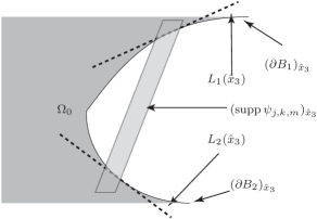
Figure 6: Case 2c. A 2D cross sections of $\mathop{\operator@font supp}\nolimits\psi_{\lambda}$ and the two discontinuity surfaces $\partial B_{1}$ and $\partial B_{2}$.

Case 2c

Without loss of generality, we may assume that $(\hat{x}_{1},\hat{x}_{2},0)$ and $(\hat{x}^{\prime}_{1},\hat{x}^{\prime}_{2},0)$ belong to $\partial B_{1}\cap\mathop{\operator@font supp}\nolimits{\psi_{j,k,m}}\cap{\mathcal{Q}}_{j,p}$ and $\partial B_{2}\cap\mathop{\operator@font supp}\nolimits{\psi_{j,k,m}}\cap{\mathcal{Q}}_{j,p}$ respectively for some $\hat{x}_{1},\hat{x}_{2},\hat{x}^{\prime}_{1},\hat{x}^{\prime}_{2}\in\mathbb{R}$. Note that for a shear index $k=(k_{1},k_{2})$ and scale $j\geq 0$ fixed, we have by a simple counting argument that

$$\#\left\lvert\bigcap_{i=1}^{2}\{m\in\mathbb{Z}^{3}:\operatorname{int}(\mathop{\operator@font supp}\nolimits{\psi_{j,k,m}})\cap\partial B_{i}\cap{\mathcal{Q}}_{j,p}\neq\emptyset\}\right\rvert\\ \leq C\min_{i=1,2}\left\{{|k_{i}+2^{j(\alpha-1)/2}s_{i}|+1}\right\}$$ (42)

where $s_{1}=\partial^{(1,0)}E_{1}(\hat{x}_{2},0)$ and $s_{2}=\partial^{(0,1)}E_{2}(\hat{x}^{\prime}_{2},0)$. For each $\hat{x}_{3}\in[0,2^{-j/2}]$, we define the 2D slice of $\mathop{\operator@font supp}\nolimits{\psi_{j,k,m}}$ by

$$(\mathop{\operator@font supp}\nolimits{\psi_{j,k,m}})_{\hat{x}_{3}}=\{(x_{1},x_{2},\hat{x}_{3}):(x_{1},x_{2},\hat{x}_{3})\in\mathop{\operator@font supp}\nolimits{\psi_{j,k,m}}\}.$$

We will now estimate the following 2D integral over $(\mathop{\operator@font supp}\nolimits{\psi_{j,k,m}})_{\hat{x}_{3}}$

$$I_{j,k,m}(\hat{x}_{3})=\int_{(\mathop{\operator@font supp}\nolimits{\psi_{j,k,m}})_{\hat{x}_{3}}}f(x_{1},x_{2},\hat{x}_{3})\psi_{j,k,m}(x_{1},x_{2},\hat{x}_{3})\mathrm{d}x_{1}\mathrm{d}x_{2}.$$ (43)

This integral above gives us the worst decay rate when the 2D support $(\mathop{\operator@font supp}\nolimits{\psi_{j,k,m}})_{\hat{x}_{3}}$ meets both edge curves, see Figure 6. Therefore, we may assume that for each $\hat{x}_{3}$ fixed, the set $(\mathop{\operator@font supp}\nolimits{\psi_{j,k,m}})_{\hat{x}_{3}}$ intersects two edge curves

$$(\partial B_{i})_{\hat{x}_{3}}=\{(x_{1},x_{2},\hat{x}_{3}):(x_{1},x_{2},\hat{x}_{3})\in\partial B_{i}\cap{\mathcal{Q}}_{j,p}\}\quad\text{for}\,\,i=1,2.$$

By a similar argument as in Section 8.2, one can linearize the two curves $(\partial B_{1})_{\hat{x}_{3}}$ and $(\partial B_{2})_{\hat{x}_{3}}$ within $(\mathop{\operator@font supp}\nolimits{\psi_{j,k,m}})_{\hat{x}_{3}}$. In other words, we now replace the discontinuity curves $(\partial B_{1})_{\hat{x}_{3}}$ and $(\partial B_{2})_{\hat{x}_{3}}$ by

$$L_{i}(\hat{x}_{3})=\{(s_{i}(\hat{x}_{3})(x_{2}-\hat{x}_{2})+\hat{x}_{1},x_{2},\hat{x}_{3})\in{\mathcal{Q}}_{j,p}\cap(\mathop{\operator@font supp}\nolimits{\psi_{j,k,m}})_{\hat{x}_{3}}:x_{2}\in\mathbb{R}\}$$

where

$$s_{i}(\hat{x}_{3})=\frac{\partial E_{i}(\hat{x}_{2},\hat{x}_{3})}{\partial x_{2}}\qquad\text{for some}\,\,(\hat{x}_{1},\hat{x}_{2},\hat{x}_{3})\in(\partial B_{i})_{\hat{x}_{3}}\,\,\text{and}\,\,i=1,2.$$

Further, we may assume that the tangent lines $L_{i}(\hat{x}_{3})$ on $(\mathop{\operator@font supp}\nolimits{\psi_{j,k,m}})_{\hat{x}_{3}}$ do not intersect each other. In particular, one can take secant lines instead of the tangent lines if necessary. The truncation error for the linearization with the secant line instead of linearization with the tangent line would not change our estimates for $\#\left\lvert\Lambda(\varepsilon)\right\rvert$. Now, on each 2D support $(\mathop{\operator@font supp}\nolimits{\psi_{j,k,m}})_{\hat{x}_{3}}$, we have a 2D piecewise smooth function

$$f(x_{1},x_{2},\hat{x}_{3})=f_{0}(x_{1},x_{2},\hat{x}_{3})\chi_{\Omega_{0}}+f_{1}(x_{1},x_{2},\hat{x}_{3})\chi_{\Omega_{1}}$$

where $f_{0},f_{1}\in C^{\beta}$ and $\Omega_{0},\Omega_{1}$ are disjoint subsets of $[0,2^{-j/2}]^{2}$ as in Figure 6. Observe that

$$f=f_{0}\chi_{\Omega_{0}}+f_{1}\chi_{\Omega_{1}}=(f_{0}-f_{1})\chi_{\Omega_{0}}+f_{1}$$

on ${\mathcal{Q}}_{j,p}\cap(\mathop{\operator@font supp}\nolimits{\psi_{j,k,m}})_{\hat{x}_{3}}$. By Proposition 18, the optimal rate of sparse approximations can be achieved for the smooth part $f_{1}$. Thus, it is sufficient to consider the first term $(f_{0}-f_{1})\chi_{\Omega_{0}}$ in the equation above. Therefore, we may assume that $f=g_{0}\chi_{\Omega_{0}}$ with a 2D function $g_{0}\in C^{\beta}$ on ${\mathcal{Q}}_{j,p}\cap(\mathop{\operator@font supp}\nolimits{\psi_{j,k,m}})_{\hat{x}_{3}}$. Note that the discontinuities of the function $f$ lie on the two edge curves $L_{i}(\hat{x}_{3})$ for $i=1,2$ on ${\mathcal{Q}}_{j,p}\cap(\mathop{\operator@font supp}\nolimits{\psi_{j,k,m}})_{\hat{x}_{3}}$. Applying the same linearized estimates as in Section 8.1 for each of edge curves $L_{i}(\hat{x}_{3})$, we obtain

$$|I_{j,k,m}(\hat{x}_{3})|\lesssim\max_{i=1,2}\left\{{\frac{2^{-j\alpha/4}}{(1+|k_{1}+2^{j(\alpha-1)/2}s_{i}(\hat{x}_{3})|)^{\alpha+1}}}\right\}.$$

By similar arguments as in (36), we can replace $s_{i}(\hat{x}_{3})$ by a universal choice $s_{i}$ for $i=1,2$ independent of $\hat{x}_{3}$. Since $\hat{x}_{3}\in[0,2^{-j/2}]$, this yields

$$|\langle\psi_{j,k,m},f\rangle|\lesssim\max_{i=1,2}\biggl{\{}\frac{2^{-j\frac{\alpha+2}{4}}}{(1+|\hat{k}_{i}|)^{\alpha+1}}\biggr{\}},$$ (44)

where $\hat{k}_{i}=k_{1}+2^{j(\alpha-1)/2}s_{i}$ for $i=1,2$ as usual. Also, we note that the number of dyadic boxes ${\mathcal{Q}}_{j,p}$ containing two distinct discontinuity surfaces is bounded above by $2^{j/2}$ times a constant independent of scale $j$. Moreover, there are a total of $\lceil 2^{j\frac{\alpha-1}{2}}\rceil+1$ shear indices with respect to the parameter $k_{2}$. Let us define

$$K_{j}(\varepsilon)=\left\{{k_{1}\in\mathbb{Z}}:{\max_{i=1,2}\bigl{\{}{(1+|\hat{k}_{i}|)^{-(\alpha+1)}2^{-j\frac{\alpha+2}{4}}}\bigr{\}}>\varepsilon}\right\}.$$

By (42) and (44), we have

$$\#\left\lvert\Lambda(\varepsilon)\right\rvert\lesssim\sum_{j=0}^{\frac{4}{\alpha+2}\log{(\varepsilon^{-1})}}2^{j/2}2^{j\frac{\alpha-1}{2}}\sum_{k_{1}\in K_{j}(\varepsilon)}\min_{i=1,2}\bigl{\{}{1+|\hat{k}_{i}|}\bigr{\}}.$$

Without loss of generality, we may assume $|\hat{k}_{1}|\leq|\hat{k}_{2}|$. Then

$$\#\left\lvert\Lambda(\varepsilon)\right\rvert\lesssim\sum_{j=0}^{\frac{4}{\alpha+2}\log{(\varepsilon^{-1})}}2^{j/2}2^{j\frac{\alpha-1}{2}}\sum_{k_{1}\in K_{j}(\varepsilon)}(1+|\hat{k}_{1}|)\lesssim\varepsilon^{-\frac{2}{\alpha+2}}\sum_{j=0}^{\frac{4}{\alpha+2}}2^{j\frac{\alpha^{2}-2}{2(\alpha+1)}}\lesssim\varepsilon^{-\frac{4}{\alpha+2}}.$$

Letting $N=\#\left\lvert\Lambda(\varepsilon)\right\rvert$, we therefore have that $\varepsilon\lesssim N^{-\frac{\alpha+2}{4}}$. This implies that

$$\left\lVert f-f_{N}\right\rVert_{L^{2}}\lesssim\sum_{n>N}\left\lvert c(f)^{\ast}_{n}\right\rvert^{2}\lesssim N^{-\alpha/2},$$

and this completes the proof.

Case 2d

Let $\partial\Gamma$ be the edge curve in which two discontinuity surfaces $\partial B_{1}$ and $\partial B_{2}$ meet inside $\operatorname{int}(\mathop{\operator@font supp}\nolimits{\psi_{j,k,m}})$. Let us assume that the edge curve $\partial\Gamma$ is given by $(E_{1}(x_{2},\rho(x_{2})),x_{2},\rho(x_{2}))$ with some smooth function $\rho\in C^{\alpha}(\mathbb{R})$. The other case, $(E_{1}(\rho(x_{3}),x_{3}),\rho(x_{3}),x_{3})$ can be handled in similar way. Without loss of generality, we may assume that the edge curve $\partial\Gamma$ passes through the origin and that $(0,0,0)\in\mathop{\operator@font supp}\nolimits{\psi_{j,k,m}}$. Let $\kappa=\rho^{\prime}(0)$, and we now consider the case $|\kappa|\leq 1$.

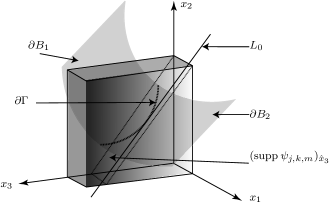
Figure 7: Case 2d. The support of $\psi_{\lambda}$ intersecting the two $C^{\alpha}$ discontinuity surfaces $\partial B_{1}$, $\partial B_{2}$ and the 1D edge curve $\partial\Gamma$, where the two patches $\partial B_{1}$ and $\partial B_{2}$ meet. The 2D cross section $(\mathop{\operator@font supp}\nolimits{\psi_{j,k,m}})_{\hat{x}_{3}}$ is indicated; it is seen as a tangent plane to $\partial\Gamma$.

The other case, $\left\lvert\kappa\right\rvert>1$, can be handled by switching the role of variables $x_{2}$ and $x_{3}$. Let us consider the tangent line $L_{0}$ to $\partial\Gamma$ at the origin. We have

$$L_{0}:\frac{x_{1}}{(s_{1}+\kappa s_{2})}=x_{2}=\frac{x_{3}}{\kappa},\,\,\,\text{where}\,\,s_{1}=\tfrac{\partial E_{1}(0,0)}{\partial x_{2}}\,\,\text{and}\,\,s_{2}=\tfrac{\partial E_{1}(0,0)}{\partial x_{3}}.$$

For each $\hat{x}_{3}\in[0,2^{-j/2}]$ fixed, define

$$(\mathop{\operator@font supp}\nolimits{\psi_{j,k,m}})_{\hat{x}_{3}}=\{(x_{1},x_{2},\kappa x_{2}+\hat{x}_{3})\in\mathop{\operator@font supp}\nolimits{\psi_{j,k,m}}:x_{1},x_{2}\in\mathbb{R}\}.$$

Also, let

$$s^{1}_{1}(\hat{x}_{3})=\tfrac{\partial E_{1}(\hat{x}_{2},\hat{x}_{3})}{\partial x_{2}},\;s^{1}_{2}(\hat{x}_{3})=\tfrac{\partial E_{1}(\hat{x}_{2},\hat{x}_{3})}{\partial x_{3}},\;s^{2}_{1}(\hat{x}_{3})=\tfrac{\partial E_{2}(\hat{x}^{\prime}_{2},\hat{x}_{3})}{\partial x_{2}},\;s^{2}_{1}(\hat{x}_{3})=\tfrac{\partial E_{2}(\hat{x}^{\prime}_{2},\hat{x}_{3})}{\partial x_{2}}$$

for some $\hat{x}_{2},\hat{x}^{\prime}_{2}\in\mathbb{R}$ such that

$$(E_{1}(\hat{x}_{2},\hat{x}_{3}),\hat{x}_{2},\hat{x}_{3}) \in\partial B_{1}\cap(\mathop{\operator@font supp}\nolimits{\psi_{j,k,m}})_{\hat{x}_{3}}$$ (45)

and

$$(E_{1}(\hat{x}^{\prime}_{2},\hat{x}_{3}),\hat{x}^{\prime}_{2},\hat{x}_{3}) \in\partial B_{2}\cap(\mathop{\operator@font supp}\nolimits{\psi_{j,k,m}})_{\hat{x}_{3}}.$$ (46)

If such a point $\hat{x}_{2}$ (or $\hat{x}^{\prime}_{2}$) does not exist, there will be no discontinuity curve on $(\mathop{\operator@font supp}\nolimits{\psi_{j,k,m}})_{\hat{x}_{3}}$ which leads to a better decay of the 2D surface integrals of the form (43). Therefore, we may assume conditions (45) and (45) holds for any $\hat{x}_{3}\in[0,2^{-j/2}]$. For $k_{2}$ fixed, let $\hat{k}_{1}=(k_{1}+\kappa k_{2})+2^{j\frac{\alpha-1}{2}}(s_{1}+\kappa s_{2})$. Applying a similar counting argument as in Section 9, for the shear index $k=(\hat{k}_{1},k_{2})$ fixed, we obtain an upper bound for the number of shearlets $\psi_{j,k,m}$ intersecting $\partial\Gamma$ inside ${\mathcal{Q}}_{j,p}$ as follows:

$$\#\left\lvert\{(j,k,m):\operatorname{int}(\mathop{\operator@font supp}\nolimits{\psi_{j,k,m}})\cap{\mathcal{Q}}_{j,p}\cap\partial\Gamma\neq\emptyset\}\right\rvert\leq C(|\hat{k}_{1}|+1).$$ (47)

Notice that there exists a region ${\mathcal{P}}$ such that the following assertions hold:

1. ${\mathcal{P}}$ contains $\partial\Gamma$ inside $\mathop{\operator@font supp}\nolimits{\psi_{j,k,m}}\cap{\mathcal{Q}}_{j,p}$.

2. ${\mathcal{P}}\subset\{(x_{1},x_{2},\kappa x_{2}+t)\in\mathop{\operator@font supp}\nolimits{\psi_{j,k,m}}:0\leq t\leq b\}\cap\mathop{\operator@font supp}\nolimits{\psi_{j,k,m}}$ for some $b\geq 0$.

Here, we choose the smallest $b$ so that (ii) holds. For each $\hat{x}_{3}\in[0,2^{-j/2}]$ fixed, let $H_{\hat{x}_{3}}=\{(x_{1},x_{2},\kappa x_{2}+\hat{x}_{3}):x_{1},x_{2}\in\mathbb{R}\}$. Applying a similar argument as in the proof of Theorem 19 to each of the 2D cross sections ${\mathcal{P}}\cap H_{\hat{x}_{3}}$ of ${\mathcal{P}}$, we obtain

$$\operatorname{vol}{({\mathcal{P}})}\lesssim 2^{-j\frac{\alpha}{2}}\Bigl{(}\frac{1}{|\hat{k}_{1}|2^{j/2}}\Bigr{)}^{\alpha+1}.$$ (48)

Figure 7 shows the 2D cross section of ${\mathcal{P}}$. Let us now estimate the decay rate of shearlet coefficients $\langle f,\psi_{j,k,m}\rangle$. Using (48),

$$\Bigl{|}\int_{\mathbb{R}^{3}}f(x)\psi_{j,k,m}(x)\mathrm{d}x\Bigr{|} \leq \Bigl{|}\int_{{\mathcal{P}}}f(x)\psi_{j,k,m}(x)\mathrm{d}x\Bigr{|}+\Bigl{|}\int_{{\mathcal{P}}^{c}}f(x)\psi_{j,k,m}(x)\mathrm{d}x\Bigr{|}$$ (49)

$$\leq C\frac{2^{-j(\frac{3\alpha}{4})}}{(1+|\hat{k}_{1}|)^{\alpha+1}}+\Bigl{|}\int_{{\mathcal{P}}^{c}}f(x)\psi_{j,k,m}(x)\mathrm{d}x\Bigr{|}$$

Next, we compute the second integral $\int_{{\mathcal{P}}^{c}}f(x)\psi_{j,k,m}(x)\mathrm{d}x$ in (49). For each $\hat{x}_{3}\in[0,2^{-j/2}]$, define

$$(\mathop{\operator@font supp}\nolimits{\psi_{j,k,m}})_{\hat{x}_{3}}=H_{\hat{x}_{3}}\cap\mathop{\operator@font supp}\nolimits{\psi_{j,k,m}}\cap{\mathcal{P}}^{c}.$$

Again, we assume that on each 2D cross section $(\mathop{\operator@font supp}\nolimits{\psi_{j,k,m}})_{\hat{x}_{3}}$ there are two edge curves $\partial B_{1}\cap H_{\hat{x}_{3}}$ and $\partial B_{2}\cap H_{\hat{x}_{3}}$ since we otherwise could obtain a better decay rate of $\langle f,\psi_{j,k,m}\rangle$. As we did in the previous case, we compute the 2D surface integral $I_{j,k,m}(\hat{x}_{3})$ over the cross section $(\mathop{\operator@font supp}\nolimits{\psi_{j,k,m}})_{\hat{x}_{3}}$ defined as in (43). Applying a similar linearization argument as in Section 8.2, we can now replace the two edge curves $\partial B_{i}\cap H_{\hat{x}_{3}}$ for $i=1,2$ by two tangent lines as follows:

$$L_{1}(\hat{x}_{3})=\{{((s^{1}_{1}(\hat{x}_{3})+\kappa s^{1}_{2}(\hat{x}_{3}))x_{2}+\hat{x}_{1},x_{2}+\hat{x}_{2},\kappa x_{2}+\hat{x}_{3})\in\mathbb{R}^{3}}:{x_{2}\in\mathbb{R}}\}$$

and

$$L_{2}(\hat{x}_{3})=\{{((s^{2}_{1}(\hat{x}_{3})+\kappa s^{2}_{2}(\hat{x}_{3}))x_{2}+\hat{x}^{\prime}_{1},x_{2}+\hat{x}^{\prime}_{2},\kappa x_{2}+\hat{x}_{3})\in\mathbb{R}^{3}}:{x_{2}\in\mathbb{R}}\}.$$

Here, the points $\hat{x}_{1},\hat{x}_{2},\hat{x}^{\prime}_{1}$, and $\hat{x}^{\prime}_{2}$ are defined as in (45) and (46), and we may assume that the two lines $L_{1}(\hat{x}_{3})$ and $L_{2}(\hat{x}_{3})$ do not intersect each other within $(\mathop{\operator@font supp}\nolimits{\psi_{j,k,m}})_{\hat{x}_{3}}$; otherwise, we can take secant lines instead as argued in the previous case. Let ${\mathcal{Q}}_{\hat{x}_{3}}$ be the projection of $(\mathop{\operator@font supp}\nolimits{\psi_{j,k,m}})_{\hat{x}_{3}}$ onto the $x_{1}x_{2}$ plane. By the assumptions on $\psi$, we have

$$I_{j,k,m}(\hat{x}_{3}) = \sqrt{1+{\kappa^{2}}}\int_{{{\mathcal{Q}}}_{\hat{x}_{3}}}f(x_{1},x_{2},\kappa x_{2}+\hat{x}_{3})\psi_{j,k,m}(x_{1},x_{2},\kappa x_{2}+\hat{x}_{3})\mathrm{d}x_{2}\mathrm{d}x_{1}$$

$$= 2^{j\frac{\alpha+2}{4}}\sqrt{1+{\kappa^{2}}}\int_{{{\mathcal{Q}}}_{\hat{x}_{3}}}f(x_{1},x_{2},\kappa x_{2}+\hat{x}_{3})$$

$$\phantom{\sqrt{1+{\kappa^{2}}}}g^{0}_{\kappa,2^{j/2}\hat{x}_{3}}\Bigl{(}2^{j\alpha/2}x_{1}+2^{j/2}(k_{1}+k_{2}\kappa)x_{2}+2^{j/2}k_{2}\hat{x}_{3},2^{j/2}x_{2}\Bigr{)}\mathrm{d}x_{2}\mathrm{d}x_{1}$$

The integral above is of the same type as in (29) except for the $\hat{x}_{3}$ translation parameter. The function $f(x_{1},x_{2},\kappa x_{2}+\hat{x}_{3})$ has singularities lying on the projection of the lines $L_{1}(\hat{x}_{3})$ and $L_{2}(\hat{x}_{3})$ onto the $x_{1}x_{2}$ plane which do not intersect inside $\operatorname{int}({\mathcal{Q}}_{\hat{x}_{3}})$. Therefore, we can apply the linearized estimate as in the proof of Theorem 19 and obtain

$$|I_{j,k,m}(\hat{x}_{3})|\leq C\max_{i=1,2}\left\{{2^{-j\frac{\alpha}{4}}{\Bigl{(}1+|(k_{1}+\kappa k_{2})+2^{j\frac{\alpha-1}{2}}(s^{i}_{1}(\hat{x}_{3})+\kappa s^{i}_{2}(\hat{x}_{3}))|\Bigr{)}^{-\alpha-1}}}\right\}.$$

By a similar argument as in (36), we can now replace $s^{i}_{i^{\prime}}(\hat{x}_{3})$ by universal choices $s_{i}$ for $i,i^{\prime}=1,2$ respectively, in the equation above. This implies

$$\Bigl{|}\int_{{\mathcal{P}}^{c}}f(x)\psi_{j,k,m}(x)\mathrm{d}x\Bigr{|}\leq C\frac{2^{-j\frac{\alpha+2}{4}}}{(1+|\hat{k}_{1}|)^{\alpha+1}}.$$ (50)

Therefore, from (49), (50), we obtain

$$|\langle f,\psi_{j,k,m}\rangle|\leq C\frac{2^{-j\frac{\alpha+2}{4}}}{(1+|\hat{k}_{1}|)^{\alpha+1}}.$$ (51)

In this case, the number of all dyadic boxes ${\mathcal{Q}}_{j,p}$ containing two distinct discontinuity surfaces is bounded above by $2^{j/2}$ up to a constant independent of scale $j$, and there are shear indices $\lceil 2^{j\frac{\alpha-1}{2}}\rceil+1$ with respect to $k_{2}$. Let us define

$$K_{j}(\varepsilon)=\left\{{k_{1}\in\mathbb{Z}}:{(1+|\hat{k}_{1}|)^{-(\alpha+1)}2^{-j\frac{\alpha+2}{4}}>\varepsilon}\right\}.$$

Finally, we now estimate $\#\left\lvert\Lambda(\varepsilon)\right\rvert$ using (47) and (51).

$$\#\left\lvert\Lambda(\varepsilon)\right\rvert\leq C\sum_{j=0}^{\frac{4}{\alpha+2}\log{(\varepsilon^{-1})}}2^{j\frac{\alpha-1}{2}}\,2^{j/2}\sum_{k_{1}\in K_{j}(\varepsilon)}(1+|\hat{k}_{1}|)\leq C\varepsilon^{-\frac{4}{\alpha+2}}$$

which provides the sought approximation rate.

Case 2e

In this case, we assume that $f=f_{0}\chi_{\Omega_{0}}+f_{1}\chi_{\Omega_{1}}$ with $f_{0},f_{1}\in C^{\beta}$, and that there are $L$ discontinuity surfaces $\partial B_{1},\dots\partial B_{L}$ inside $\operatorname{int}(\mathop{\operator@font supp}\nolimits{\psi_{j,k,m}})$ so that each of the discontinuity surfaces is parametrized by $x_{1}=E_{i}(x_{2},x_{3})$ with $E_{i}\in C^{\alpha}$ for $i=1,\dots,L$. For each $\hat{x}_{3}\in\left[{0},{2^{-j/2}}\right]$, let us consider the 2D support

$$(\mathop{\operator@font supp}\nolimits{\psi_{j,k,m}})_{\hat{x}_{3}}=\{(x_{1},x_{2},\hat{x}_{3})\in\mathop{\operator@font supp}\nolimits{\psi_{j,k,m}}:x_{1},x_{2}\in\mathbb{R}\}.$$

On each 2D slice $(\mathop{\operator@font supp}\nolimits{\psi_{j,k,m}})_{\hat{x}_{3}}$, let

$$\partial\Gamma^{i}_{\hat{x}_{3}}=(\mathop{\operator@font supp}\nolimits{\psi_{j,k,m}})_{\hat{x}_{3}}\cap\partial B_{i}\qquad\text{for}\,\,i=1,\dots,L.$$

Observe that there are at most two distinct curves $\partial\Gamma^{i}_{\hat{x}_{3}}$ and $\partial\Gamma^{i^{\prime}}_{\hat{x}_{3}}$ on $(\mathop{\operator@font supp}\nolimits{\psi_{j,k,m}})_{\hat{x}_{3}}$ for some $i,i^{\prime}=1,\dots,L$. We can assume that there are such two edge curves $\partial\Gamma^{1}_{\hat{x}_{3}}$ and $\partial\Gamma^{2}_{\hat{x}_{3}}$ for each $\hat{x}_{3}\in[0,2^{-j/2}]$ since we otherwise could obtain better decay rate of the shearlet coefficients $|\langle f,\psi_{j,k,m}\rangle|$. From this, we may assume that for each $\hat{x}_{3}$, there exist $(\hat{x}_{1},\hat{x}_{2},\hat{x}_{3})$ and $(\hat{x}^{\prime}_{1},\hat{x}^{\prime}_{2},\hat{x}_{3})\in\operatorname{int}(\mathop{\operator@font supp}\nolimits{\psi_{j,k,m}})$ such that $(\hat{x}_{1},\hat{x}_{2},\hat{x}_{3})\in\partial\Gamma^{1}(\hat{x}_{3})$ and $(\hat{x}^{\prime}_{1},\hat{x}^{\prime}_{2},\hat{x}_{3})\in\partial\Gamma^{2}(\hat{x}_{3})$. We then set:

$$s^{1}_{1}(\hat{x}_{3})=\tfrac{\partial E_{1}(\hat{x}_{1},\hat{x}_{2})}{\partial x_{2}}\qquad\text{and}\qquad s^{2}_{1}(\hat{x}_{3})=\tfrac{\partial E_{2}(\hat{x}_{1},\hat{x}^{\prime}_{2})}{\partial x_{2}}.$$

Applying a similar linearization argument as in Section 8.2, we can replace the two edge curves by two tangent lines (or secant lines) as follows:

$$L^{1}(\hat{x}_{3})=\left\{{(s^{1}_{1}(\hat{x}_{3})x_{2}+\hat{x}_{1},x_{2}+\hat{x}_{2},\hat{x}_{3})}:{x_{2}\in\mathbb{R}}\right\}$$

and

$$L^{2}(\hat{x}_{3})=\left\{{(s^{2}_{1}(\hat{x}_{3})x_{2}+\hat{x}^{\prime}_{1},x_{2}+\hat{x}^{\prime}_{2},\hat{x}_{3})}:{x_{2}\in\mathbb{R}}\right\}.$$

Here, we may assume that the two tangent lines $L^{1}(\hat{x}_{3})$ and $L^{2}(\hat{x}_{3})$ do not intersect inside $(\mathop{\operator@font supp}\nolimits{\psi_{j,k,m}})_{\hat{x}_{3}}\cap{\mathcal{Q}}_{j,p}$ for each $\hat{x}_{3}$. In fact, the number of shearlet supports $\psi_{j,k,m}$ intersecting ${\mathcal{Q}}_{j,p}\cap\partial B_{1}\cap\dots\cap\partial B_{L}$, so that there are two tangent lines $L^{1}(\hat{x}_{3})$ and $L^{2}(\hat{x}_{3})$ meeting each other inside $(\mathop{\operator@font supp}\nolimits{\psi_{j,k,m}})_{\hat{x}_{3}}$ for some $\hat{x}_{3}$, is bounded by some constant $C$ independent of scale $j$. Those shearlets $\psi_{j,k,m}$ are covered by Case 2f, and we may therefore simply ignore those shearlets in this case. Using a similar argument as in the estimate of (29), one can then estimate $I_{j,k,m}(\hat{x}_{3})$ defined as in (43) as follows:

$$I_{j,k,m}(\hat{x}_{3})\leq C\min_{i=1,2}\left\{{\frac{2^{-j\frac{\alpha}{4}}}{(1+|k_{1}+2^{j\frac{\alpha-1}{2}}s^{i}_{1}(\hat{x}_{3})|)^{\alpha+1}}}\right\}.$$

Again, applying similar arguments as in (36), we may replace the slopes $s^{i}_{1}(\hat{x}_{3})$ and $s^{i^{\prime}}_{1}(\hat{x}_{3})$ by universal choices $s^{i}_{1}(0)$ and $s^{i^{\prime}}_{1}(0)$, respectively. This gives

$$|\langle f,\psi_{j,k,m}\rangle|\leq C\max_{i=1,\dots,L}\left\{{\frac{2^{-j\frac{\alpha+2}{4}}}{(1+|\hat{k}^{i}_{1}|)^{\alpha+1}}}\right\},$$ (52)

where $\hat{k}^{i}_{1}=s^{i}_{1}(0)2^{j\frac{\alpha-1}{2}}+k_{1}$ for $i=1,\dots,L$. Further, applying a similar counting argument as in Section 9, for $k=(k_{1},k_{2})$ and $j\geq 0$ fixed, we have

$$\#\left\lvert\left\{{(j,k,m)}\right\}{\operatorname{int}(\mathop{\operator@font supp}\nolimits{\psi_{j,k,m}})\cap\partial B_{1}\cap\dots\cap\partial B_{L}\cap{\mathcal{Q}}_{j,p}\neq\emptyset}\right\rvert\\ \leq C\min_{i=1,\dots,L}\bigl{\{}{1+|\hat{k}^{i}_{1}|}\bigr{\}}.$$ (53)

In this case, the number of all dyadic boxes ${\mathcal{Q}}_{j,p}$ containing more than two distinct discontinuity surfaces is bounded by some constant independent of scale $j$, and there are $\lceil 2^{j\frac{\alpha-1}{2}}\rceil+1$ shear indices with respect to $k_{2}$. Let us define

$$K_{j}(\varepsilon)=\left\{{k_{1}\in\mathbb{Z}}:{\max_{i=1,\dots,L}\bigl{\{}{(1+|\hat{k}^{i}_{1}|)^{-(\alpha+1)}2^{-j\frac{\alpha+2}{4}}}\bigr{\}}>\varepsilon}\right\}.$$

Finally, using (52) and (53), we see that

$$|\Lambda(\varepsilon)|\leq C\sum_{j=0}^{\frac{4}{\alpha+2}\log{(\varepsilon^{-1})}}2^{j\frac{\alpha-1}{2}}\sum_{k_{1}\in K_{j}(\varepsilon)}\min_{i=1,\dots,L}\bigl{\{}{1+|\hat{k}^{i}_{1}|}\bigr{\}}\leq C\varepsilon^{-\frac{2}{\alpha+4}}.$$

This proves Case 2e.

Case 2f

In this case, since the total number of shear parameters $k=(k_{1},k_{2})$ is bounded by a constant times $2^{j}$ for each $j\geq 0$, it follows that

$$\#\left\lvert\Lambda_{j,p}(\varepsilon)\right\rvert\leq C\cdot 2^{j}.$$

Since there are only finitely many corner points with its number not depending on scale $j\geq 0$, we have

$$\#\left\lvert\Lambda(\varepsilon)\right\rvert\leq C\cdot\sum_{j=0}^{\frac{4}{\alpha+2}\log_{2}{(\varepsilon^{-1})}}2^{j}\leq C\cdot\varepsilon^{-\frac{4}{\alpha+2}},$$

which, in turn, implies the optimal sparse approximation rate for Case 2f. This completes the proof of Theorem 14.

11 Extensions

11.1 Smoothness parameters $\alpha$ and $\beta$

Our 3D image model class ${\mathcal{E}}_{\alpha}^{\beta}(\mathbb{R}^{3})$ depends primarily of the two parameters $\alpha$ and $\beta$. The particular choice of scaling matrix is essential for the nearly optimal approximation results in Section 6, but any choice of scaling matrix basically only allows us to handle one parameter. This of course poses a problem if one seeks optimality results for all $\alpha,\beta\in\left({1},{2}\right]$. We remark that our choice of scaling matrix exactly “fits” the smoothness parameter of the discontinuity surface $\alpha$, which exactly is the crucial parameter when $\beta\geq\alpha$ as assumed in our optimal sparsity results. It is unclear whether one can circumvent the problem of having “too” many parameters, and thereby prove sparse approximation results as in Section 6 for the case $\beta<\alpha\leq 2$.

For $\alpha>2$ we can, however, not expect shearlet systems $SH{(\phi,\psi,\tilde{\psi},\breve{\psi})}$ to deliver optimal sparse approximations. The heuristic argument is as follows. For simplicity let us only consider shearlet elements associated with the pyramid pair ${\mathcal{P}}$. Suppose that the discontinuity surface is $C^{2}$. Locally we can assume the surface will be of the form $x_{1}=E(x_{2},x_{3})$ with $E\in C^{2}$. Consider a Taylor expansion of $E$ at $(x_{2}^{\prime},x_{3}^{\prime})$:

$$E(x_{2},x_{3})=E(x_{1}^{\prime},x_{2}^{\prime})+\begin{pmatrix}\partial^{(1,0)}E(x_{1}^{\prime},x_{2}^{\prime})&\partial^{(0,1)}E(x_{1}^{\prime},x_{2}^{\prime})\end{pmatrix}\begin{pmatrix}x_{2}\\ x_{3}\end{pmatrix}\\ +\begin{pmatrix}x_{2}&x_{3}\end{pmatrix}\begin{pmatrix}\partial^{(2,0)}E(\xi_{1},\xi_{2})&\partial^{(1,1)}E(\xi_{1},\xi_{2})\\ \partial^{(1,1)}E(\xi_{1},\xi_{2})&\partial^{(0,2)}E(\xi_{1},\xi_{2})\end{pmatrix}\begin{pmatrix}x_{2}\\ x_{3}\end{pmatrix}.$$ (54)

Intuitively, we need our shearlet elements $\psi_{j,k,m}$ to capture the geometry of $\partial B$. For the term $E(x_{1}^{\prime},x_{2}^{\prime})$ we use the translation parameter $m\in\mathbb{Z}^{3}$ to locate the shearlet element near the expansion point $p:=(E(x_{1}^{\prime},x_{2}^{\prime}),x_{2}^{\prime},x_{3}^{\prime})$. Next, we “rotate” the element $\psi_{j,k,m}$ using the sharing parameter $k\in\mathbb{Z}^{2}$ to align the shearlet normal with the normal of the tangent plane of $\partial B$ in $p$; the direction of the tangent is of course governed by $\partial^{(1,0)}E(x_{1}^{\prime},x_{2}^{\prime})$ and $\partial^{(0,1)}E(x_{1}^{\prime},x_{2}^{\prime})$. Since the last parameter $j\in\mathbb{N}_{0}$ is a multi-scale parameter, we do not have more parameters available to capture the geometry of $\partial B$. Note that the scaling matrix $A_{2^{j}}$ can, for $\alpha=2$, be written as

$$A_{2^{j}}=\begin{pmatrix}2^{j}&0&0\\ 0&2^{j/2}&0\\ 0&0&2^{j/2}\end{pmatrix}=\begin{pmatrix}2&0&0\\ 0&2^{1/2}&0\\ 0&0&2^{1/2}\end{pmatrix}^{j}.$$

The shearlet element will therefore have support in a parallelopiped with side lengths $2^{-j}$ , $2^{-j/2}$ and $2^{-j/2}$ in directions of the $x_{1}$, $x_{2}$, and $x_{3}$ axis, respectively. Since

$$\left\lvert x_{2}x_{3}\right\rvert\leq 2^{-j},x_{2}^{2}\leq 2^{-j},\text{ and }x_{3}^{2}\leq 2^{-j},$$

for $\left\lvert x_{2}\right\rvert,\left\lvert x_{3}\right\rvert\leq 2^{-j/2}$, we see that the paraboliodal scaling gives shearlet elements of a size that exactly fits the Hermitian term in (54). If $\partial B\in C^{\alpha}$ for $1<\alpha\leq 2$, that is, $E\in C^{\alpha}$ for $1<\alpha\leq 2$, we in a similar way see that our choice of scaling matrix exactly fits the last term in the corresponding Taylor expansion. Now, if the discontinuity surface is smoother than $C^{2}$, that is, $\partial B\in C^{\alpha}$ for $\alpha>2$, say $\partial B\in C^{3}$, we could include one more term in the Taylor expansion (54), but we do not have any more free parameters to adapt to this increased information. Therefore, we will arrive at the same (and now non-optimal) approximation rate as for $\partial B\in C^{2}$. We conclude that for $\alpha>2$ we will need representation systems with not only a directional characteristic, but also some type of curvature characteristic.

For $\alpha<1$, we do not have proper directional information about the anisotropic discontinuity, in particular, we do not have a tangential plane at every point on the discontinuity surface. This suggests that this kind of anisotropic phenomenon should not be investigated with directional representation systems. For the boarder-line case $\alpha=1$, our analysis shows that wavelet systems should be used for sparse approximations.

11.2 Needle-like shearlets

In place of $A_{2^{j}}=\mathop{\operator@font diag}\nolimits{(2^{\alpha j/2},2^{j/2},2^{j/2})}$, one could also use the scaling matrix $A_{2^{j}}=\mathop{\operator@font diag}\nolimits{(2^{j\alpha/2},2^{j\alpha/2},2^{j/2})}$ with similar changes for $\tilde{A}_{2^{j}}$ and $\breve{A}_{2^{j}}$. This would lead to needle-like shearlet elements instead of the plate-like elements considered in this paper. As Theorem 14 in Section 6.1 showed, the plate-like shearlet systems are able to deliver almost optimal sparse approximation even in the setting of cartoon-like images with certain types of 1D singularities. This might suggest that needle-like shearlet systems are not necessary, at least not for sparse approximation issues. Furthermore, the tiling of the frequency space becomes increasingly complicated in the situation of needle-like shearlet systems which yields frames with less favorable frame constants. However, in non-asymptotic analyses, e.g., image separation, a combined needle-like and plate-like shearlet system might be useful.

11.3 Future work

For $\alpha<2$, the obtained approximation error rate is only near-optimal since it differs by $\tau(\alpha)$ from the true optimal rate. It is unclear whether one can get rid of the $\tau(\alpha)$ exponent (perhaps replacing it with a poly-$\log$ factor) by using better estimates in the proofs in Section 8. More general, it is also future work to determine whether shearlet systems with $\alpha,\beta\in\left({1},{2}\right]$ provide nearly or truly optimal sparse approximations of all $f\in{\mathcal{E}}_{\alpha}^{\beta}(\mathbb{R}^{3})$. To answer this question, one would, however, need to develop a completely new set of techniques. This would mean that the approximation error would decay as $O(N^{-\min\{\alpha/2,2\beta/3\}})$ as $N\to\infty$, perhaps with additional poly-log factors or a small polynomial factor.

Acknowledgements

The first and third author acknowledge support from DFG Grant SPP-1324, KU 1446/13. The first author also acknowledges support from DFG Grant KU 1446/14.

Appendix A Estimates

The following estimates are used repeatedly in Section 5 and follows by direct verification. For $t=2^{-m}$, i.e., $-\log_{2}t=m$, $m\in\mathbb{N}_{0}:=\mathbb{N}\cup\{0\}$, we have

$$\sum_{\left\{{j\in\mathbb{N}_{0}}:{2^{-j}\geq t}\right\}}(2^{-j})^{-\iota}=\sum_{j=0}^{{-\log_{2}t}}(2^{\iota})^{j}=\frac{t^{-\iota}-2^{-\iota}}{1-2^{-\iota}}\qquad\text{for $\iota\neq 0$,}$$

$$\sum_{\left\{{j\in\mathbb{N}_{0}}:{2^{-j}\leq t}\right\}}(2^{-j})^{\iota}=\sum_{j={-\log_{2}t}}^{\infty}(2^{-\iota})^{j}=\frac{t^{\iota}}{1-2^{-\iota}}\qquad\text{for $\iota>0$,}$$

For $t\in\left({0},{1}\right]$, we have $\left\lceil-\log_{2}t\right\rceil\in\mathbb{N}_{0}$ and therefore

$$\sum_{\left\{{j\in\mathbb{N}_{0}}:{2^{-j}\geq t}\right\}}(2^{-j})^{-\iota}=\sum_{j=0}^{\left\lfloor-\log_{2}t\right\rfloor}(2^{\iota})^{j}\leq\frac{t^{-\iota}-2^{-\iota}}{1-2^{-\iota}}\qquad\text{for $\iota>0$,}$$ (55)

$$\sum_{\left\{{j\in\mathbb{N}_{0}}:{2^{-j}\leq t}\right\}}(2^{-j})^{\iota}=\sum_{j=\left\lceil-\log_{2}t\right\rceil}^{\infty}(2^{-\iota})^{j}\leq\frac{t^{\iota}}{1-2^{-\iota}}\qquad\text{for $\iota>0$,}$$ (56)

where we have used that $2^{\left\lfloor-\log_{2}t\right\rfloor}\leq t^{-1}$ and $2^{-\left\lceil-\log_{2}t\right\rceil}=2^{\left\lfloor\log_{2}t\right\rfloor}\leq t$. For $t>1$ we finally have that

$$\sum_{\left\{{j\in\mathbb{N}_{0}}:{2^{-j}\geq t}\right\}}(2^{-j})^{-\iota}=0\quad\text{and}\quad\sum_{\left\{{j\in\mathbb{N}_{0}}:{2^{-j}\leq t}\right\}}(2^{-j})^{\iota}=\sum_{j=0}^{\infty}(2^{-\iota})^{j}=\frac{1}{1-2^{-\iota}}.$$ (57)

Appendix B Proof of Proposition 8

We start by estimating $\Gamma(2\omega)$, and will use this later to derive the claimed upper estimate for $R(c)$. For brevity we will use $K_{j}:=\left[{-\lceil 2^{j(\alpha-1)/2}\rceil},{\lceil 2^{j(\alpha-1)/2}\rceil}\right]$ and $k\in K_{j}$ to mean $k_{1},k_{2}\in K_{j}$. By definition it then follows that

$$\Gamma(2\omega_{1},2\omega_{2},2\omega_{3})\\ \leq\operatorname*{ess\,sup}_{\xi\in{\mathbb{R}^{3}}}\;\sum_{j\geq 0}\sum_{k\in K_{j}}\left\lvert\hat{\psi}\left(2^{-j\alpha/2}\xi_{1},k_{1}2^{-j\alpha/2}\xi_{1}+2^{-j/2}\xi_{2},k_{2}2^{-j\alpha/2}\xi_{1}+2^{-j/2}\xi_{3}\right)\right\rvert\\ \cdot\left\lvert\hat{\psi}\left(2^{-j\alpha/2}\xi_{1}+2\omega_{1},k_{1}2^{-j\alpha/2}\xi_{1}+2^{-j/2}\xi_{2}+2\omega_{2},k_{2}2^{-j\alpha/2}\xi_{1}+2^{-j/2}\xi_{3}+2\omega_{3}\right)\right\rvert.$$

For each $(\omega_{1},\omega_{2},\omega_{3})\in{\mathbb{R}^{3}}\setminus\left\{{0}\right\}$, we first split the sum over the index set $\mathbb{N}_{0}$ into index sets $J_{1}=\left\{{j\geq 0}:{\lvert 2^{-j\alpha/2}\xi_{1}\rvert\leq\left\lVert\omega\right\rVert_{\infty}}\right\}$ and $J_{2}=\left\{{j\geq 0}:{\lvert 2^{-j\alpha/2}\xi_{1}\rvert>\left\lVert\omega\right\rVert_{\infty}}\right\}$. We denote these sums by $I_{1}$ and $I_{2}$, respectively. In other words, we have that

$$\Gamma(2\omega_{1},2\omega_{2},2\omega_{3})\leq\operatorname*{ess\,sup}\limits_{\xi\in{\mathbb{R}^{3}}}(I_{1}+I_{2}),$$ (58)

where

$$I_{1}=\sum_{j\in J_{1}}\sum_{k\in K_{j}}\Bigl{\lvert}\hat{\psi}\bigl{(}2^{-j\alpha/2}\xi_{1},k_{1}2^{-j\alpha/2}\xi_{1}+2^{-j/2}\xi_{2},k_{2}2^{-j\alpha/2}\xi_{1}+2^{-j/2}\xi_{3}\bigr{)}\Bigr{\rvert}\\ \cdot\Bigl{\lvert}\hat{\psi}\bigl{(}2^{-j\alpha/2}\xi_{1}+2\omega_{1},k_{1}2^{-j\alpha/2}\xi_{1}+2^{-j/2}\xi_{2}+2\omega_{2},k_{2}2^{-j\alpha/2}\xi_{1}+2^{-j/2}\xi_{3}+2\omega_{3}\bigr{)}\Bigr{\rvert}$$

and

$$I_{2}=\sum_{j\in J_{2}}\sum_{k\in K_{j}}\left\lvert\hat{\psi}\left(2^{-j\alpha/2}\xi_{1},k_{1}2^{-j\alpha/2}\xi_{1}+2^{-j/2}\xi_{2},k_{2}2^{-j\alpha/2}\xi_{1}+2^{-j/2}\xi_{3}\right)\right\rvert\\ \cdot\left\lvert\hat{\psi}\left(2^{-j\alpha/2}\xi_{1}+2\omega_{1},k_{1}2^{-j\alpha/2}\xi_{1}+2^{-j/2}\xi_{2}+2\omega_{2},k_{2}2^{-j\alpha/2}\xi_{1}+2^{-j/2}\xi_{3}+2\omega_{3}\right)\right\rvert.$$

The next step consists of estimating $I_{1}$ and $I_{2}$, but we first introduce some useful inequalities which will be needed later. Recall that $\delta>2\gamma>6$, and $q,q^{\prime},r,s$ are positive constants satisfying $q^{\prime},r,s\in\left({0},{q}\right)$. Further, let $\gamma^{\prime\prime}=\gamma-\gamma^{\prime}$ for an arbitrarily fixed $\gamma^{\prime}$ satisfying $1<\gamma^{\prime}<\gamma-2$. Let $\iota>\gamma>3$. Then we have the following inequalities for $x,y,z\in\mathbb{R}$.

$$\min\{1,|qx|^{\iota}\}\min\{1,|ry|^{-\gamma}\}\leq\min\{1,|qx|^{\iota-\gamma}\}\min\left\{1,|(qx)^{-1}ry|^{-\gamma}\right\},$$ (59)

$$\min\{1,|x|^{-\gamma}\}\min\left\{1,\left|\frac{1+z}{x+y}\right|^{\gamma}\right\}\leq 2^{\gamma^{\prime\prime}}|y|^{-\gamma^{\prime\prime}}\min\{1,|x|^{-\gamma^{\prime}}\}\max\{1,|1+z|^{\gamma^{\prime\prime}}\},$$ (60)

$$\min\{1,|qx|^{\iota-\gamma}\}\min\{1,|q^{\prime}x|^{-\gamma}\}|x|^{\gamma^{\prime\prime}}\leq(q^{\prime})^{-\gamma^{\prime\prime}},$$ (61)

and

$$\min\{1,|qx|^{\iota-\gamma}\}\min\{1,|q^{\prime}x|^{-\gamma}\}|x|^{\gamma^{\prime\prime}}\leq(q^{\prime})^{-\gamma^{\prime\prime}}\min\{1,|qx|^{\iota-\gamma+\gamma^{\prime\prime}}\}\min\{1,|q^{\prime}x|^{-\gamma^{\prime}}\}.$$ (62)

We fix $\xi\in\mathbb{R}^{3}$ and start with $I_{1}$. By the decay assumptions (10) on $\hat{\psi}$, it follows directly that

$$I_{1}\leq\sum_{j\in J_{1}}\min\left\{{|q2^{-j\alpha/2}\xi_{1}|^{\delta},1}\right\}\min\left\{{|q^{\prime}2^{-j\alpha/2}\xi_{1}|^{-\gamma},1}\right\}\\ \cdot\min\left\{{\left\lvert q(2^{-j\alpha/2}\xi_{1}+2\omega_{1})\right\rvert^{\delta},1}\right\}\min\left\{{\left\lvert q^{\prime}(2^{-j\alpha/2}\xi_{1}+2\omega_{1})\right\rvert^{-\gamma},1}\right\}\\ \sum_{k_{1}\in K_{j}}\min\bigl{\{}{\bigl{\lvert}r(k_{1}2^{-j\alpha/2}\xi_{1}+2^{-j/2}\xi_{2})\bigr{\rvert}^{-\gamma}}\bigr{\}}\min\bigl{\{}{\bigl{\lvert}r(k_{1}2^{-j\alpha/2}\xi_{1}+2^{-j/2}\xi_{2}+2\omega_{2})\bigr{\rvert}^{-\gamma}}\bigr{\}}\\ \sum_{k_{2}\in K_{j}}\min\bigl{\{}{\bigl{\lvert}s(k_{2}2^{-j\alpha/2}\xi_{1}\!+2^{-j/2}\xi_{3})\bigr{\rvert}^{-\gamma}}\bigr{\}}\min\bigl{\{}{\bigl{\lvert}s(k_{2}2^{-j\alpha/2}\xi_{1}\!+2^{-j/2}\xi_{3}+2\omega_{3})\bigr{\rvert}^{-\gamma}}\bigr{\}}.$$

Further, using inequality (59) with $\iota=\delta$ and $\iota=2\delta$ twice,

$$I_{1}\leq\sum_{j\in J_{1}}\min\left\{{|q2^{-j\alpha/2}\xi_{1}|^{\delta-2\gamma},1}\right\}\min\left\{{|q^{\prime}2^{-j\alpha/2}\xi_{1}|^{-\gamma},1}\right\}\\ \cdot\min\left\{{\left\lvert q(2^{-j\alpha/2}\xi_{1}+2\omega_{1})\right\rvert^{\delta-2\gamma},1}\right\}\min\left\{{\left\lvert q^{\prime}(2^{-j\alpha/2}\xi_{1}+2\omega_{1})\right\rvert^{-\gamma},1}\right\}\\ \sum_{k_{1}\in\mathbb{Z}}\min\left\{{\left\lvert\frac{r}{q}\left(k_{1}+2^{j\frac{\alpha-1}{2}}\tfrac{\xi_{2}}{\xi_{1}}\right)\right\rvert^{-{\gamma}},1}\right\}\\ \min\left\{{\left\lvert\frac{r}{q}\left[\left(\frac{2\omega_{2}}{2^{-j\alpha/2}\xi_{1}}\right)+\left(k_{1}+2^{j\frac{\alpha-1}{2}}\tfrac{\xi_{2}}{\xi_{1}}\right)\right]\right\rvert^{{-\gamma}}\left\lvert 1+\frac{2\omega_{1}}{2^{-j\alpha/2}\xi_{1}}\right\rvert^{\gamma},1}\right\}\\ \sum_{k_{2}\in\mathbb{Z}}\min\left\{{\left\lvert\frac{s}{q}\left(k_{2}+2^{j\frac{\alpha-1}{2}}\tfrac{\xi_{3}}{\xi_{1}}\right)\right\rvert^{-{\gamma}},1}\right\}\\ \min\left\{{\left\lvert\frac{r}{q}\left[\left(\frac{2\omega_{3}}{2^{-j\alpha/2}\xi_{1}}\right)+\left(k_{2}+2^{j\frac{\alpha-1}{2}}\tfrac{\xi_{3}}{\xi_{1}}\right)\right]\right\rvert^{{-\gamma}}\left\lvert 1+\frac{2\omega_{1}}{2^{-j\alpha/2}\xi_{1}}\right\rvert^{\gamma},1}\right\},$$ (63)

where we, e.g., in the sum over $k_{1}$, have used paraphrases as

$$\frac{r(k_{1}2^{-j\alpha/2}\xi_{1}+2^{-j/2}\xi_{2})}{q2^{-j\alpha/2}\xi_{1}}=\frac{r}{q}\left(k_{1}+2^{j\frac{\alpha-1}{2}}\tfrac{\xi_{2}}{\xi_{1}}\right)$$

and

$$\frac{r(k_{1}2^{-j\alpha/2}\xi_{1}+2^{-j/2}\xi_{2}+2\omega_{2})}{q(2^{-j\alpha/2}\xi_{1}+2\omega_{1})}=\frac{r}{q}\Biggl{[}\left(\frac{2\omega_{2}}{2^{-j\alpha/2}\xi_{1}}\right)\\ +\left(k_{1}+2^{j\frac{\alpha-1}{2}}\tfrac{\xi_{2}}{\xi_{1}}\right)\Biggr{]}\left(1+\frac{2\omega_{1}}{2^{-j\alpha/2}\xi_{1}}\right)^{-1}.$$

We now consider the following three cases: $\left\lVert\omega\right\rVert_{\infty}=\left\lvert\omega_{1}\right\rvert\geq\left\lvert 2^{-j\alpha/2}\xi_{1}\right\rvert$, $\left\lVert\omega\right\rVert_{\infty}=|\omega_{2}|\geq\left\lvert 2^{-j\alpha/2}\xi_{1}\right\rvert$, and $\left\lVert\omega\right\rVert_{\infty}=|\omega_{3}|\geq\left\lvert 2^{-j\alpha/2}\xi_{1}\right\rvert$. Notice that these three cases indeed do include all possible relations between $\omega$ and $\xi_{1}$.

Case I

We assume that $\left\lVert\omega\right\rVert_{\infty}=\left\lvert\omega_{1}\right\rvert\geq\left\lvert 2^{-j\alpha/2}\xi_{1}\right\rvert$, hence $\left\lvert 2^{-j\alpha/2}\xi_{1}+2\omega_{1}\right\rvert\geq\left\lvert\omega_{1}\right\rvert$. Using the trivial estimates $\min\{{\left\lvert q(2^{-j\alpha/2}\xi_{1}+2\omega_{1})\right\rvert^{\delta-2\gamma},1}\}\leq 1$,

$$\min\left\{{\left\lvert\frac{r}{q}\left[\left(\frac{2\omega_{2}}{2^{-j\alpha/2}\xi_{1}}\right)+\left(k_{1}+2^{j\frac{\alpha-1}{2}}\tfrac{\xi_{2}}{\xi_{1}}\right)\right]\right\rvert^{{-\gamma}}\left\lvert 1+\frac{2\omega_{1}}{2^{-j\alpha/2}\xi_{1}}\right\rvert^{\gamma},1}\right\}\leq 1,$$

and analogue estimates for the sum over $k_{2}$, we can continue (63),

$$I_{1}\leq\sum_{j\in J_{1}}\min\left\{{|q2^{-j\alpha/2}\xi_{1}|^{\delta-2\gamma},1}\right\}\min\left\{{|q^{\prime}2^{-j\alpha/2}\xi_{1}|^{-\gamma},1}\right\}\left\lvert q^{\prime}(2^{-j\alpha/2}\xi_{1}+2\omega_{1})\right\rvert^{-\gamma}\\ \sum_{k_{1}\in\mathbb{Z}}\min\left\{{\left\lvert\frac{r}{q}\left(k_{1}+2^{j\frac{\alpha-1}{2}}\tfrac{\xi_{2}}{\xi_{1}}\right)\right\rvert^{-{\gamma}},1}\right\}\sum_{k_{2}\in\mathbb{Z}}\min\left\{{\left\lvert\frac{s}{q}\left(k_{2}+2^{j\frac{\alpha-1}{2}}\tfrac{\xi_{3}}{\xi_{1}}\right)\right\rvert^{-{\gamma}},1}\right\}.$$

Our assumption $\left\lVert\omega\right\rVert_{\infty}=\left\lvert\omega_{1}\right\rvert$ implies $\left\lvert q^{\prime}(2^{-j\alpha/2}\xi_{1}+2\omega_{1})\right\rvert^{-\gamma}\leq\left\lVert q^{\prime}\omega\right\rVert_{\infty}^{-\gamma}$. Therefore,

$$I_{1}\leq\left\lVert q^{\prime}\omega\right\rVert_{\infty}^{-\gamma}\sum_{j\in J_{1}}\min\left\{{\left\lvert q2^{-j\alpha/2}\xi_{1}\right\rvert^{\delta-2\gamma},1}\right\}\min\left\{{\left\lvert q^{\prime}2^{-j\alpha/2}\xi_{1}\right\rvert^{-\gamma},1}\right\}\\ \frac{q}{r}\sum_{k_{1}\in\mathbb{Z}}\frac{r}{q}\min\left\{{\left\lvert\frac{r}{q}\left(k_{1}+2^{j\frac{\alpha-1}{2}}\tfrac{\xi_{2}}{\xi_{1}}\right)\right\rvert^{-{\gamma}},1}\right\}\cdot\frac{q}{s}\sum_{k_{2}\in\mathbb{Z}}\frac{s}{q}\min\left\{{\left\lvert\frac{s}{q}\left(k_{2}+2^{j\frac{\alpha-1}{2}}\tfrac{\xi_{3}}{\xi_{1}}\right)\right\rvert^{-{\gamma}},1}\right\}.$$

By the estimate (14) with $y=r/q\leq 1$ (and $y=s/q\leq 1$) as constant, we can bound the sum over $k_{1}$ (and $k_{2}$), leading to

$$I_{1}\leq\left\lVert q^{\prime}\omega\right\rVert_{\infty}^{-\gamma}\sum_{j\in J_{1}}\min\left\{{\left\lvert q2^{-j\alpha/2}\xi_{1}\right\rvert^{\delta-2\gamma},1}\right\}\min\left\{{\left\lvert q^{\prime}2^{-j\alpha/2}\xi_{1}\right\rvert^{-\gamma},1}\right\}\,\frac{q}{r}C(\gamma)\,\frac{q}{s}C(\gamma).$$

Taking the supremum over $\xi_{1}=\eta_{1}/q\in\mathbb{R}$ and using equations (55) and (56) as in the proof of Proposition 7 yields

$$I_{1} \leq\frac{q^{2}}{rs}C(\gamma)^{2}\left\lVert q^{\prime}\omega\right\rVert_{\infty}^{-\gamma}\sup_{\eta_{1}\in\mathbb{R}}\sum_{j\in J_{1}}\min\left\{{\left\lvert 2^{-j\alpha/2}\eta_{1}\right\rvert^{\delta-2\gamma},1}\right\}\min\left\{{\left\lvert q^{\prime}q^{-1}2^{-j\alpha/2}\eta_{1}\right\rvert^{-\gamma},1}\right\}$$

$$\leq\frac{q^{2}}{rs}C(\gamma)^{2}\left\lVert q^{\prime}\omega\right\rVert_{\infty}^{-\gamma}\Bigl{(}\left\lceil\frac{2}{\alpha}\log_{2}\Bigl{(}\frac{q}{q^{\prime}}\Bigr{)}\right\rceil+\frac{1}{1-2^{-\delta+2\gamma}}+1\Bigr{)}.$$ (64)

Case II

We now assume that $\left\lVert\omega\right\rVert_{\infty}=\left\lvert\omega_{2}\right\rvert\geq\left\lvert 2^{-j\alpha/2}\xi_{1}\right\rvert$. For $\gamma=\gamma^{\prime}+\gamma^{\prime\prime}$, $\gamma>\gamma^{\prime}+2>3$, $\gamma^{\prime}>1$, $\gamma^{\prime\prime}>2$ by (60)

$$\min\left\{{\left\lvert\frac{r}{q}\left(k_{1}+2^{j\frac{\alpha-1}{2}}\tfrac{\xi_{2}}{\xi_{1}}\right)\right\rvert^{-{\gamma}},1}\right\}\min\left\{{\left\lvert\frac{1+\frac{2\omega_{1}}{2^{-j\alpha/2}\xi_{1}}}{\frac{r}{q}\left(\frac{2\omega_{2}}{2^{-j\alpha/2}\xi_{1}}+k_{1}+2^{j\frac{\alpha-1}{2}}\frac{\xi_{2}}{\xi_{1}}\right)}\right\rvert^{\gamma},1}\right\}\\ \leq 2^{\gamma^{\prime\prime}}\left\lvert\frac{r}{q}\frac{2\omega_{2}}{2^{-j\alpha/2}\xi_{1}}\right\rvert^{-\gamma^{\prime\prime}}\min\left\{{\left\lvert\frac{r}{q}\left(k_{1}+2^{j\frac{\alpha-1}{2}}\tfrac{\xi_{2}}{\xi_{1}}\right)\right\rvert^{-{\gamma^{\prime}}},1}\right\}\max{\left\{{\left\lvert 1+\frac{2\omega_{1}}{2^{-j\alpha/2}\xi_{1}}\right\rvert^{\gamma^{\prime\prime}},1}\right\}}$$

Applied to (63) this yields

$$I_{1}\leq\sum_{j\in J_{1}}\min\left\{{|q2^{-j\alpha/2}\xi_{1}|^{\delta-2\gamma},1}\right\}\min\left\{{|q^{\prime}2^{-j\alpha/2}\xi_{1}|^{-\gamma},1}\right\}\\ \cdot\min\left\{{\left\lvert q(2^{-j\alpha/2}\xi_{1}+2\omega_{1})\right\rvert^{\delta-2\gamma},1}\right\}\min\left\{{\left\lvert q^{\prime}(2^{-j\alpha/2}\xi_{1}+2\omega_{1})\right\rvert^{-\gamma},1}\right\}\\ \sum_{k_{1}\in\mathbb{Z}}2^{\gamma^{\prime\prime}}\left\lvert\frac{r}{q}\frac{2\omega_{2}}{2^{-j\alpha/2}\xi_{1}}\right\rvert^{-\gamma^{\prime\prime}}\min\left\{{\left\lvert\frac{r}{q}\left(k_{1}+2^{j\frac{\alpha-1}{2}}\tfrac{\xi_{2}}{\xi_{1}}\right)\right\rvert^{-{\gamma^{\prime}}},1}\right\}\max{\left\{{\left\lvert 1+\frac{2\omega_{1}}{2^{-j\alpha/2}\xi_{1}}\right\rvert^{\gamma^{\prime\prime}},1}\right\}}\\ \sum_{k_{2}\in\mathbb{Z}}\min\left\{{\left\lvert\frac{s}{q}\left(k_{2}+2^{j\frac{\alpha-1}{2}}\tfrac{\xi_{3}}{\xi_{1}}\right)\right\rvert^{-{\gamma}},1}\right\}.$$ (65)

Hence, by estimate (14),

$$I_{1}\leq 2^{\gamma^{\prime\prime}}\frac{q^{2}}{rs}C(\gamma)C(\gamma^{\prime})\lVert 2\tfrac{r}{q}w\rVert_{\infty}^{-\gamma^{\prime\prime}}\sum_{j\in J_{1}}\min\left\{{|q2^{-j\alpha/2}\xi_{1}|^{\delta-2\gamma},1}\right\}\min\left\{{|q^{\prime}2^{-j\alpha/2}\xi_{1}|^{-\gamma},1}\right\}\\ \cdot\min\left\{{\left\lvert q(2^{-j\alpha/2}\xi_{1}+2\omega_{1})\right\rvert^{\delta-2\gamma},1}\right\}\min\left\{{\left\lvert q^{\prime}(2^{-j\alpha/2}\xi_{1}+2\omega_{1})\right\rvert^{-\gamma},1}\right\}\\ \left\lvert{2^{-j\alpha/2}\xi_{1}}\right\rvert^{\gamma^{\prime\prime}}\max{\left\{{\left\lvert 1+\frac{2\omega_{1}}{2^{-j\alpha/2}\xi_{1}}\right\rvert^{\gamma^{\prime\prime}},1}\right\}}.$$ (66)

We further split Case II into the following two subcases: $1\leq|1+\frac{2\omega_{1}}{2^{-j\alpha/2}\xi_{1}}|$ and $1>|1+\frac{2\omega_{1}}{2^{-j\alpha/2}\xi_{1}}|$. Now, in case $1\leq|1+\frac{2\omega_{1}}{2^{-j\alpha/2}\xi_{1}}|$, then obviously

$$\left|{2^{-j\alpha/2}\xi_{1}}\right|^{\gamma^{\prime\prime}}\max\left\{1,\left|1+\frac{2\omega_{1}}{2^{-j\alpha/2}\xi_{1}}\right|^{\gamma^{\prime\prime}}\right\}\leq\left|2^{-j\alpha/2}\xi_{1}+2\omega_{1}\right|^{\gamma^{\prime\prime}},$$

which used in (66) yields

$$I_{1}\leq\frac{q^{2}}{rs}C(\gamma)C(\gamma^{\prime})\lVert\tfrac{r}{q}w\rVert_{\infty}^{-\gamma^{\prime\prime}}\sum_{j\in J_{1}}\min\left\{{|q2^{-j\alpha/2}\xi_{1}|^{\delta-2\gamma},1}\right\}\min\left\{{|q^{\prime}2^{-j\alpha/2}\xi_{1}|^{-\gamma},1}\right\}\\ \cdot\min\left\{{\left\lvert q(2^{-j\alpha/2}\xi_{1}+2\omega_{1})\right\rvert^{\delta-2\gamma},1}\right\}\min\left\{{\left\lvert q^{\prime}(2^{-j\alpha/2}\xi_{1}+2\omega_{1})\right\rvert^{-\gamma},1}\right\}\left|2^{-j\alpha/2}\xi_{1}+2\omega_{1}\right|^{\gamma^{\prime\prime}},$$

Hence, by inequality (61) with $\iota=\delta-\gamma$, i.e.,

$$\min\left\{{\left\lvert q(2^{-j\alpha/2}\xi_{1}+2\omega_{1})\right\rvert^{\delta-2\gamma},1}\right\}\min\left\{{\left\lvert q^{\prime}(2^{-j\alpha/2}\xi_{1}+2\omega_{1})\right\rvert^{-\gamma},1}\right\}\left|2^{-j\alpha/2}\xi_{1}+2\omega_{1}\right|^{\gamma^{\prime\prime}}\leq(q^{\prime})^{-\gamma^{\prime\prime}},$$

we arrive at

$$I_{1} \leq\frac{q^{2}}{rs}C(\gamma)C(\gamma^{\prime})\lVert\tfrac{q^{\prime}r}{q}w\rVert_{\infty}^{-\gamma^{\prime\prime}}\sum_{j\in J_{1}}\min\left\{{|q2^{-j\alpha/2}\xi_{1}|^{\delta-2\gamma},1}\right\}\min\left\{{|q^{\prime}2^{-j\alpha/2}\xi_{1}|^{-\gamma},1}\right\}$$

$$\leq\frac{q^{2}}{rs}C(\gamma)C(\gamma^{\prime})\lVert\tfrac{q^{\prime}r}{q}w\rVert_{\infty}^{-\gamma^{\prime\prime}}\Bigl{(}\left\lceil\frac{2}{\alpha}\log_{2}\Bigl{(}\frac{q}{q^{\prime}}\Bigr{)}\right\rceil+\frac{1}{1-2^{-\delta+2\gamma}}+1\Bigr{)}.$$ (67)

On the other hand, if $1\geq|1+\frac{2\omega_{1}}{2^{-j\alpha/2}\xi_{1}}|$, then,

$$\min\left\{{\bigl{\lvert}q(2^{-j\tfrac{\alpha}{2}}\xi_{1}+2\omega_{1})\bigr{\rvert}^{{\delta-\gamma}},1}\right\}\min\left\{{\bigl{\lvert}q^{\prime}(2^{-j\tfrac{\alpha}{2}}\xi_{1}+2\omega_{1})\bigr{\rvert}^{-\gamma},1}\right\}\max\left\{{\bigl{\lvert}1+\tfrac{2\omega_{1}}{a_{j}\xi_{1}}\bigr{\rvert}^{\gamma^{\prime\prime}},1}\right\}\leq 1,$$

for all $j\geq 0$. Hence from (66), by employing inequality (62), we arrive at

$$I_{1} \leq\frac{q^{2}}{rs}C(\gamma)C(\gamma^{\prime})\lVert\tfrac{r}{q}w\rVert_{\infty}^{-\gamma^{\prime\prime}}\sum_{j\in J_{1}}\min\left\{{|q2^{-j\tfrac{\alpha}{2}}\xi_{1}|^{\delta-2\gamma},1}\right\}\min\left\{{|q^{\prime}2^{-j\tfrac{\alpha}{2}}\xi_{1}|^{-\gamma},1}\right\}\left\lvert{2^{-j\tfrac{\alpha}{2}}\xi_{1}}\right\rvert^{\gamma^{\prime\prime}}$$

$$\leq\frac{q^{2}}{rs}C(\gamma)C(\gamma^{\prime})\lVert\tfrac{r}{q}w\rVert_{\infty}^{-\gamma^{\prime\prime}}\sum_{j\in J_{1}}(q^{\prime})^{-\gamma^{\prime\prime}}\min\left\{{|q2^{-j\tfrac{\alpha}{2}}\xi_{1}|^{\delta-2\gamma+\gamma^{\prime\prime}},1}\right\}\min\left\{{|q^{\prime}2^{-j\tfrac{\alpha}{2}}\xi_{1}|^{-\gamma^{\prime}},1}\right\}$$

$$\leq\frac{q^{2}}{rs}C(\gamma)C(\gamma^{\prime})\lVert\tfrac{q^{\prime}r}{q}w\rVert_{\infty}^{-\gamma^{\prime\prime}}\Bigl{(}\left\lceil\frac{2}{\alpha}\log_{2}\Bigl{(}\frac{q}{q^{\prime}}\Bigr{)}\right\rceil+\frac{1}{1-2^{-\delta+2\gamma-\gamma^{\prime\prime}}}+1\Bigr{)}.$$ (68)

Case III

This case is similar to Case II and the estimates from Case II hold with the obvious modifications. We therefore skip the proof.

We next estimate $I_{2}$. First, notice that the inequality (63) still holds for $I_{2}$ with the index set $J_{1}$ replaced by $J_{2}$. Therefore, we obviously have

$$I_{2}\leq\sum_{j\in J_{2}}\min\left\{{|q2^{-j\alpha/2}\xi_{1}|^{\delta-2\gamma},1}\right\}\min\left\{{|q^{\prime}2^{-j\alpha/2}\xi_{1}|^{-\gamma},1}\right\}\\ \sum_{k_{1}\in\mathbb{Z}}\min\left\{{\left\lvert\frac{r}{q}\left(k_{1}+2^{j\frac{\alpha-1}{2}}\tfrac{\xi_{2}}{\xi_{1}}\right)\right\rvert^{-{\gamma}},1}\right\}\sum_{k_{2}\in\mathbb{Z}}\min\left\{{\left\lvert\frac{s}{q}\left(k_{2}+2^{j\frac{\alpha-1}{2}}\tfrac{\xi_{3}}{\xi_{1}}\right)\right\rvert^{-{\gamma}},1}\right\},$$

by (14),

$$I_{1} \leq\frac{q^{2}}{rs}C(\gamma)^{2}\sum_{j\in J_{2}}\min\left\{{|q2^{-j\alpha/2}\xi_{1}|^{\delta-2\gamma},1}\right\}\min\left\{{|q^{\prime}2^{-j\alpha/2}\xi_{1}|^{-\gamma},1}\right\}$$

$$\leq\frac{q^{2}}{rs}C(\gamma)^{2}\left\lVert q^{\prime}\omega\right\rVert_{\infty}^{-\gamma}.$$ (69)

Summarising, using (58), (64), and (69), we have that

$$\Gamma(2\omega)\leq\frac{q^{2}}{rs}\frac{C(\gamma)^{2}}{\left\lVert q^{\prime}\omega\right\rVert_{\infty}^{\gamma}}\Bigl{(}\left\lceil\log_{2}\Bigl{(}\frac{q}{q^{\prime}}\Bigr{)}\right\rceil+\frac{1}{1-2^{-\delta+2\gamma}}+\frac{1}{1-2^{-\gamma}}\Bigr{)}+\frac{q^{2}}{rs}\frac{C(\gamma)^{2}}{\left\lVert q^{\prime}\omega\right\rVert_{\infty}^{\gamma}}\frac{1}{1-2^{-\gamma}},$$

whenever $\left\lVert\omega\right\rVert_{\infty}=\left\lvert\omega_{1}\right\rvert$, and by (67), (68), and (69),

$$\Gamma(2\omega) \leq\frac{q^{2}}{rs}\frac{C(\gamma)C(\gamma^{\prime})}{\lVert\tfrac{q^{\prime}\min\{r,s\}}{q}w\rVert_{\infty}^{\gamma^{\prime\prime}}}\Bigl{(}\frac{4}{\alpha}\left\lceil\log_{2}\Bigl{(}\frac{q}{q^{\prime}}\Bigr{)}\right\rceil+\frac{1}{1-2^{-\delta+2\gamma}}+\frac{1}{1-2^{-\delta+2\gamma-\gamma^{\prime\prime}}}+2\Bigr{)}$$

$$\phantom{\leq}+\frac{q^{2}}{rs}\frac{C(\gamma)^{2}}{\left\lVert q^{\prime}\omega\right\rVert_{\infty}^{\gamma}},$$

otherwise. We are now ready to prove the claimed estimate for $R(c)$. Define

$$\mathcal{Q}=\left\{{m\in\mathbb{Z}^{3}}:{|m_{1}|>|m_{2}|\text{ and }\left\lvert m_{1}\right\rvert>\left\lvert m_{3}\right\rvert}\right\},$$

and

$$\tilde{\mathcal{Q}}=\left\{{m\in\mathbb{Z}^{3}}:{c_{1}^{-1}|m_{1}|>c_{2}^{-1}|m_{2}|\text{ and }c_{1}^{-1}|m_{1}|>c_{2}^{-1}|m_{3}|}\right\}.$$

If $m\in\tilde{\mathcal{Q}}$, that is, if $c_{1}^{-1}|m_{1}|>c_{2}^{-1}|m_{2}|$ and $c_{1}^{-1}|m_{1}|>c_{2}^{-1}|m_{2}|$, then

$$\Gamma(\pm M_{c}^{-1}m)\leq\frac{q^{2}}{rs}\frac{C(\gamma)^{2}}{\left\lVert m\right\rVert_{\infty}^{\gamma}}\left(\frac{2c_{1}}{q^{\prime}}\right)^{\gamma}\Bigl{(}\left\lceil\log_{2}\Bigl{(}\frac{q}{q^{\prime}}\Bigr{)}\right\rceil+\frac{1}{1-2^{-\delta+2\gamma}}+\frac{2}{1-2^{-\gamma}}\Bigr{)}\\ =(T_{1}+T_{3})\left\lVert m\right\rVert_{\infty}^{-\gamma}$$

If on the other hand $m\in\tilde{\mathcal{Q}}^{c}\setminus\{0\}$, that is, if $c_{1}^{-1}|m_{1}|\leq c_{2}^{-1}|m_{2}|$ or $c_{1}^{-1}|m_{1}|\leq c_{2}^{-1}|m_{3}|$ with $m\neq 0$, then

$$\Gamma(\pm M_{c}^{-1}m)\leq\frac{q^{2}}{rs}\frac{C(\gamma)C(\gamma^{\prime})}{\lVert m\rVert_{\infty}^{\gamma^{\prime\prime}}}\left(\frac{2qc_{2}}{q^{\prime}r}\right)^{\gamma^{\prime\prime}}\Bigl{(}2\left\lceil\log_{2}\Bigl{(}\frac{q}{q^{\prime}}\Bigr{)}\right\rceil+\frac{1}{1-2^{-\delta+2\gamma}}+\frac{1}{1-2^{-\gamma}}+\\ \frac{1}{1-2^{-\delta+2\gamma-\gamma^{\prime\prime}}}+\frac{1}{1-2^{-\gamma^{\prime}}}\Bigr{)}+\frac{q^{2}}{rs}\frac{C(\gamma)^{2}}{\left\lVert m\right\rVert_{\infty}^{\gamma}}\left(\frac{2c_{1}}{q^{\prime}}\right)^{\gamma}\frac{1}{1-2^{-\gamma}}=(T_{2}+T_{3})\,\lVert m\rVert_{\infty}^{\gamma^{\prime\prime}},$$

Therefore, we obtain

$$R(c) =\sum_{m\in\mathbb{Z}^{3}\setminus\{0\}}\left(\Gamma(M_{c}^{-1}m)\,\Gamma(-M_{c}^{-1}m)\right)^{1/2}$$

$$\leq\left(\sum_{m\in\tilde{{\mathcal{Q}}}}T_{1}\|m\|^{-\gamma}_{\infty}+T_{3}\|m\|^{-\gamma}_{\infty}\right)+\left(\sum_{m\in\tilde{{\mathcal{Q}}}^{c}\backslash\{0\}}T_{2}\|m\|^{-\gamma^{\prime\prime}}_{\infty}+T_{3}\|m\|^{-\gamma}_{\infty}\right)$$ (70)

Notice that, since $\tilde{{\mathcal{Q}}}\subset{\mathcal{Q}}$,

$$\sum_{m\in\tilde{{\mathcal{Q}}}}\|m\|^{-\gamma}\leq\sum_{m\in{{\mathcal{Q}}}}\|m\|^{-\gamma}.$$

Also, we have

$$\sum_{m\in\tilde{{\mathcal{Q}}}^{c}\backslash\{0\}}\|m\|^{-\gamma^{\prime\prime}}\leq 3\min{\left\{{\left\lceil\frac{c_{1}}{c_{2}}\right\rceil,2}\right\}}\sum_{m\in{{\mathcal{Q}}^{c}\backslash\{0\}}}\|m\|^{-\gamma^{\prime\prime}}.$$

Therefore, (70) can be continued by

$$R(c)\leq T_{3}\sum_{m\in\mathbb{Z}^{3}\setminus\{0\}}\|m\|_{\infty}^{-\gamma}+T_{1}\sum_{m\in{\mathcal{Q}}}\|m\|_{\infty}^{-\gamma}+3\min{\left\{{\left\lceil\frac{c_{1}}{c_{2}}\right\rceil,2}\right\}}T_{2}\sum_{m\in{{\mathcal{Q}}^{c}\backslash\{0\}}}\|m\|^{-\gamma^{\prime\prime}}.$$

To provide an explicit estimate for the upper bound of $R(c)$, we compute $\sum_{m\in{\mathcal{Q}}}\|m\|_{\infty}^{-\gamma}$ and $\sum_{m\in{\mathcal{Q}}^{c}\backslash}\|m\|_{\infty}^{-\gamma}$ as follows:

$$\sum_{m\in\mathbb{Z}^{3}\setminus\{0\}}\left\lVert m\right\rVert_{\infty}^{-\gamma} =\sum_{d=1}^{\infty}(24d^{2}+2)d^{-\gamma}=24\zeta(\gamma-2)+2\zeta(\gamma)$$

where $(2d+1)^{3}-(2d+1)^{3}=24d^{2}+2$ is the number of lattice points in $\mathbb{Z}^{3}$ at distance $d$ (in max-norm) from origo. Further,

$$\sum_{m\in{\mathcal{Q}}}\left\lVert m\right\rVert_{\infty}^{-\gamma} =2\sum_{m_{1}=1}^{\infty}(2m_{1}-1)^{2}m_{1}^{-\gamma}=\sum_{m_{1}=1}^{\infty}(8m_{1}^{2-\gamma}-8m_{1}^{1-\gamma}+2m_{1}^{-\gamma})$$

$$=8\zeta(\gamma-2)-4\zeta(\gamma-1)+2\zeta(\gamma)$$

and

$$\sum_{m\in{\mathcal{Q}}^{c}\setminus\{0\}}\left\lVert m\right\rVert_{\infty}^{-\gamma} =24\zeta(\gamma-2)+2\zeta(\gamma)-\bigl{(}8\zeta(\gamma-2)-4\zeta(\gamma-1)+2\zeta(\gamma)\bigr{)}$$

$$=16\zeta(\gamma-2)-4\zeta(\gamma-1),$$

which completes the proof.

References

- [1] R. A. Adams, Sobolev spaces, Pure and Applied Mathematics, Vol. 65. Academic Press, New York-London, 1975.
- [2] J. P. Antoine, P. Carrette, R. Murenzi, and B. Piette, Image analysis with two-dimensional continuous wavelet transform, Signal Process. 31 (1993), 241–272.
- [3] R. H. Bamberger and M. J. T. Smith, A filter bank for the directional decomposition of images: theory and design, IEEE Trans. Signal Process. 40 (1992), 882–893.
- [4] L. Borup and M. Nielsen, Frame decomposition of decomposition spaces, J. Fourier Anal. Appl. 13 (2007), 39–70.
- [5] E. J. Candés, L. Demanet, D. Donoho, L. Ying, Fast discrete curvelet transforms, Multiscale Model. Simul. 5 (2006), 861–899.
- [6] E. J. Candés and D. L. Donoho, Curvelets – a suprisingly effective nonadaptive representation for objects with edges, in Curve and Surface Fitting: Saint-Malo 1999, edited by A. Cohen, C. Rabut, and L. L. Schumaker, Vanderbilt University Press, Nashville, TN, 2000.
- [7] E. J. Candés and D. L. Donoho, New tight frames of curvelets and optimal representations of objects with piecewise singularities, Comm. Pure and Appl. Math. 56 (2004), 216–266.
- [8] V. Chandrasekaran, M. B. Wakin, D. Baron R. G. Baraniuk, Representation and compression of multidimensional piecewise functions using surflets, IEEE Trans. Inform. Theory 55 (2009), 374–400.
- [9] S. Dahlke, G. Kutyniok, G. Steidl, and G. Teschke, Shearlet coorbit spaces and associated Banach frames, Appl. Comput. Harmon. Anal. 27 (2009), 195–214.
- [10] S. Dahlke, G. Steidl, and G. Teschke, The continuous shearlet transform in arbitrary space dimensions, J. Fourier Anal. Appl. 16 (2010), 340–364.
- [11] S. Dahlke, G. Steidl and G. Teschke, Shearlet Coorbit Spaces: Compactly Supported Ana- lyzing Shearlets, Traces and Embeddings, J. Fourier Anal. Appl., to appear.
- [12] I. Daubechies, Ten Lectures on Wavelets, SIAM, Philadelphia, 1992.
- [13] M. N. Do and M. Vetterli, The contourlet transform: an efficient directional multiresolution image representation, IEEE Trans. Image Process. 14 (2005), 2091–2106.
- [14] D. L. Donoho, Sparse components of images and optimal atomic decomposition, Constr. Approx. 17 (2001), 353–382.
- [15] K. Guo, G. Kutyniok, and D. Labate, Sparse multidimensional representations using anisotropic dilation and shear operators, in Wavelets and Splines (Athens, GA, 2005), Nashboro Press, Nashville, TN, 2006, 189–201.
- [16] K. Guo and D. Labate, Analysis and detection of surface discontinuities using the 3D continuous shearlet transform, Appl. Comput. Harmon. Anal., to appear.
- [17] K. Guo and D. Labate, Optimally sparse multidimensional representation using shearlets, SIAM J. Math Anal. 39 (2007), 298–318.
- [18] K. Guo and D. Labate, Optimally sparse representations of 3D data with surface singularities using Parseval frames of shearlets, preprint.
- [19] K. Guo and D. Labate, Optimally sparse 3D approximations using shearlet representations, Electron. Res. Announc. Math. Sci. 17 (2010), 125–137.
- [20] P. Kittipoom, G. Kutyniok, and W.-Q Lim, Construction of compactly supported shearlet frames, Constr. Approx., to appear.
- [21] G. Kutyniok and D. Labate, Construction of regular and irregular shearlets, J. Wavelet Theory and Appl. 1 (2007), 1–10.
- [22] G. Kutyniok, J. Lemvig, and W.-Q Lim, Compactly supported shearlets, in Approximation Theory XIII (San Antonio, TX, 2010), Springer, to appear.
- [23] G. Kutyniok, J. Lemvig, and W.-Q Lim, Optimally sparse approximation and shearlets, in Shearlets: Multiscale Analysis for Multivariate Data, edited by D. Labate and G. Kutyniok, Springer, to appear.
- [24] G. Kutyniok and W.-Q Lim, Compactly supported shearlets are optimally sparse, J. Approx. Theory, to appear.
- [25] D. Labate, W.-Q Lim, G. Kutyniok, and G. Weiss. Sparse multidimensional representation using shearlets, in Wavelets XI, edited by M. Papadakis, A. F. Laine, and M. A. Unser, SPIE Proc. 5914, SPIE, Bellingham, WA, 2005, 254–262,
- [26] W.-Q Lim, The discrete shearlet transform: A new directional transform and compactly supported shearlet frames, IEEE Trans. Image Process. 19 (2010), 1166–1180.
- [27] Y. Lu and M.N. Do, Multidimensional directional filterbanks and surfacelets, IEEE Trans. Image Process. 16 (2007) 918–931.
- [28] E. L. Pennec and S. Mallat, Sparse geometric image representations with bandelets, IEEE Trans. Image Process. 14 (2005), 423–438.
- [29] E. P. Simoncelli, W. T. Freeman, E. H. Adelson, D. J. Heeger, Shiftable multiscale transforms, IEEE Trans. Inform. Theory 38 (1992), 587–607.