LSRN: A Parallel Iterative Solver for Strongly
Over- or Under-Determined Systems

Abstract

We describe a parallel iterative least squares solver named LSRN that is based on random normal projection. LSRN computes the min-length solution to $\min_{x\in\mathbb{R}^{n}}\|Ax-b\|_{2}$, where $A\in\mathbb{R}^{m\times n}$ with $m\gg n$ or $m\ll n$, and where $A$ may be rank-deficient. Tikhonov regularization may also be included. Since $A$ is only involved in matrix-matrix and matrix-vector multiplications, it can be a dense or sparse matrix or a linear operator, and LSRN automatically speeds up when $A$ is sparse or a fast linear operator. The preconditioning phase consists of a random normal projection, which is embarrassingly parallel, and a singular value decomposition of size $\lceil\gamma\min(m,n)\rceil\times\min(m,n)$, where $\gamma$ is moderately larger than $1$, e.g., $\gamma=2$. We prove that the preconditioned system is well-conditioned, with a strong concentration result on the extreme singular values, and hence that the number of iterations is fully predictable when we apply LSQR or the Chebyshev semi-iterative method. As we demonstrate, the Chebyshev method is particularly efficient for solving large problems on clusters with high communication cost. Numerical results demonstrate that on a shared-memory machine, LSRN outperforms LAPACK’s DGELSD on large dense problems, and MATLAB’s backslash (SuiteSparseQR) on sparse problems. Further experiments demonstrate that LSRN scales well on an Amazon Elastic Compute Cloud cluster.

xxx/xxxxxxxxx

1 Introduction

Randomized algorithms have become indispensable in many areas of computer science, with applications ranging from complexity theory to combinatorial optimization, cryptography, and machine learning. Randomization has also been used in numerical linear algebra (for instance, the initial vector in the power iteration is chosen at random so that almost surely it has a nonzero component along the direction of the dominant eigenvector), yet most well-developed matrix algorithms, e.g., matrix factorizations and linear solvers, are deterministic. In recent years, however, motivated by large data problems, very nontrivial randomized algorithms for very large matrix problems have drawn considerable attention from researchers, originally in theoretical computer science and subsequently in numerical linear algebra and scientific computing. By randomized algorithms, we refer in particular to random sampling and random projection algorithms [7, 22, 8, 21, 1]. For a comprehensive overview of these developments, see the review of Mahoney [17], and for an excellent overview of numerical aspects of coupling randomization with classical low-rank matrix factorization methods, see the review of Halko, Martinsson, and Tropp [13].

Here, we consider high-precision solving of linear least squares (LS) problems that are strongly over- or under-determined, and possibly rank-deficient. In particular, given a matrix $A\in\mathbb{R}^{m\times n}$ and a vector $b\in\mathbb{R}^{m}$, where $m\gg n$ or $m\ll n$ and we do not assume that $A$ has full rank, we wish to develop randomized algorithms to compute accurately the unique min-length solution to the problem

$$\text{minimize}_{x\in\mathbb{R}^{n}}\quad\|Ax-b\|_{2}.$$ (1)

If we let $r=\mathop{\operator@font rank}\nolimits(A)\leq\min(m,n)$, then recall that if $r<n$ (the LS problem is under-determined or rank-deficient), then (1) has an infinite number of minimizers. In that case, the set of all minimizers is convex and hence has a unique element having minimum length. On the other hand, if $r=n$ so the problem has full rank, there exists only one minimizer to (1) and hence it must have the minimum length. In either case, we denote this unique min-length solution to (1) by $x^{*}$. That is,

$$x^{*}=\arg\min\|x\|_{2}\quad\text{subject to}\quad x\in\arg\min_{z}\|Az-b\|_{2}.$$ (2)

LS problems of this form have a long history, tracing back to Gauss, and they arise in numerous applications. The demand for faster LS solvers will continue to grow in light of new data applications and as problem scales become larger and larger.

In this paper, we describe an LS solver called LSRN for these strongly over- or under-determined, and possibly rank-deficient, systems. LSRN uses random normal projections to compute a preconditioner matrix such that the preconditioned system is provably extremely well-conditioned. Importantly for large-scale applications, the preconditioning process is embarrassingly parallel, and it automatically speeds up with sparse matrices and fast linear operators. LSQR [20] or the Chebyshev semi-iterative (CS) method [11] can be used at the iterative step to compute the min-length solution within just a few iterations. We show that the latter method is preferred on clusters with high communication cost.

Because of its provably-good conditioning properties, LSRN has a fully predictable run-time performance, just like direct solvers, and it scales well in parallel environments. On large dense systems, LSRN is faster than LAPACK’s DGELSD for strongly over-determined problems, and is much faster for strongly under-determined problems, although solvers using fast random projections, like Blendenpik [1], are still slightly faster in both cases. On sparse systems, LSRN runs significantly faster than competing solvers, for both the strongly over- or under-determined cases.

In section 2 we describe existing deterministic LS solvers and recent randomized algorithms for the LS problem. In section 3 we show how to do preconditioning correctly for rank-deficient LS problems, and in section 4 we introduce LSRN and discuss its properties. Section 5 describes how LSRN can handle Tikhonov regularization for both over- and under-determined systems, and in section 6 we provide a detailed empirical evaluation illustrating the behavior of LSRN.

2 Least squares solvers

In this section we discuss related work, including deterministic direct and iterative methods as well as recently developed randomized methods, for computing solutions to LS problems, and we discuss how our results fit into this broader context.

2.1 Deterministic methods

It is well known that $x^{*}$ in (2) can be computed using the singular value decomposition (SVD) of $A$. Let $A=U\Sigma V^{\raisebox{0.62997pt}{\hbox{\tiny$T$}}}$ be the economy-sized SVD, where $U\in\mathbb{R}^{m\times r}$, $\Sigma\in\mathbb{R}^{r\times r}$, and $V\in\mathbb{R}^{n\times r}$. We have $x^{*}=V\Sigma^{-1}U^{\raisebox{0.62997pt}{\hbox{\tiny$T$}}}b$. The matrix $V\Sigma^{-1}U^{\raisebox{0.62997pt}{\hbox{\tiny$T$}}}$ is the Moore-Penrose pseudoinverse of $A$, denoted by $A^{\dagger}$. The pseudoinverse is defined and unique for any matrix. Hence we can simply write $x^{*}=A^{\dagger}b$. The SVD approach is accurate and robust to rank-deficiency.

Another way to solve (2) is using a complete orthogonal factorization of $A$. If we can find orthonormal matrices $Q\in\mathbb{R}^{m\times r}$ and $Z\in\mathbb{R}^{n\times r}$, and a matrix $T\in\mathbb{R}^{r\times r}$, such that $A=QTZ^{\raisebox{0.62997pt}{\hbox{\tiny$T$}}}$, then the min-length solution is given by $x^{*}=ZT^{-1}Q^{\raisebox{0.62997pt}{\hbox{\tiny$T$}}}b$. We can treat SVD as a special case of complete orthogonal factorization. In practice, complete orthogonal factorization is usually computed via rank-revealing QR factorizations, making $T$ a triangular matrix. The QR approach is less expensive than SVD, but it is slightly less robust at determining the rank of $A$.

A third way to solve (2) is by computing the min-length solution to the normal equation $A^{\raisebox{0.62997pt}{\hbox{\tiny$T$}}}Ax=A^{\raisebox{0.62997pt}{\hbox{\tiny$T$}}}b$, namely

$$x^{*}=(A^{\raisebox{0.62997pt}{\hbox{\tiny$T$}}}A)^{\dagger}A^{\raisebox{0.62997pt}{\hbox{\tiny$T$}}}b=A^{\raisebox{0.62997pt}{\hbox{\tiny$T$}}}(AA^{\raisebox{0.62997pt}{\hbox{\tiny$T$}}})^{\dagger}b.$$ (3)

It is easy to verify the correctness of (3) by replacing $A$ by its economy-sized SVD $U\Sigma V^{\raisebox{0.62997pt}{\hbox{\tiny$T$}}}$. If $r=\min(m,n)$, a Cholesky factorization of either $A^{\raisebox{0.62997pt}{\hbox{\tiny$T$}}}A$ (if $m\geq n$) or $AA^{\raisebox{0.62997pt}{\hbox{\tiny$T$}}}$ (if $m\leq n$) solves (3) nicely. If $r<\min(m,n)$, we need the eigensystem of $A^{\raisebox{0.62997pt}{\hbox{\tiny$T$}}}A$ or $AA^{\raisebox{0.62997pt}{\hbox{\tiny$T$}}}$ to compute $x^{*}$. The normal equation approach is the least expensive among the three direct approaches we have mentioned, especially when $m\gg n$ or $m\ll n$, but it is also the least accurate one, especially on ill-conditioned problems. See Chapter 5 of Golub and Van Loan [10] for a detailed analysis.

Instead of these direct methods, we can use iterative methods to solve (1). If all the iterates $\{x^{(k)}\}$ are in $\text{range}(A^{\raisebox{0.62997pt}{\hbox{\tiny$T$}}})$ and if $\{x^{(k)}\}$ converges to a minimizer, it must be the minimizer having minimum length, i.e., the solution to (2). This is the case when we use a Krylov subspace method starting with a zero vector. For example, the conjugate gradient (CG) method on the normal equation leads to the min-length solution (see Paige and Saunders [19]). In practice, CGLS [15], LSQR [20] are preferable because they are equivalent to applying CG to the normal equation in exact arithmetic but they are numerically more stable. Other Krylov subspace methods such as the CS method [11] and LSMR [9] can solve (1) as well.

Importantly, however, it is in general hard to predict the number of iterations for CG-like methods. The convergence rate is affected by the condition number of $A^{\raisebox{0.62997pt}{\hbox{\tiny$T$}}}A$. A classical result [16, p.187] states that

$$\frac{\|x^{(k)}-x^{*}\|_{A^{\raisebox{0.44998pt}{\hbox{\tiny$T$}}}A}}{\|x^{(0)}-x^{*}\|_{A^{\raisebox{0.44998pt}{\hbox{\tiny$T$}}}A}}\leq 2\left(\frac{\sqrt{\kappa(A^{\raisebox{0.62997pt}{\hbox{\tiny$T$}}}A)}-1}{\sqrt{\kappa(A^{\raisebox{0.62997pt}{\hbox{\tiny$T$}}}A)}+1}\right)^{k},$$ (4)

where $\|z\|_{A^{\raisebox{0.44998pt}{\hbox{\tiny$T$}}}A}=z^{\raisebox{0.62997pt}{\hbox{\tiny$T$}}}A^{\raisebox{0.62997pt}{\hbox{\tiny$T$}}}Az=\|Az\|^{2}$ for any $z\in\mathbb{R}^{n}$, and where $\kappa(A^{\raisebox{0.62997pt}{\hbox{\tiny$T$}}}A)$ is the condition number of $A^{\raisebox{0.62997pt}{\hbox{\tiny$T$}}}A$ under the $2$-norm. Estimating $\kappa(A^{\raisebox{0.62997pt}{\hbox{\tiny$T$}}}A)$ is generally as hard as solving the LS problem itself, and in practice the bound does not hold in any case unless reorthogonalization is used. Thus, the computational cost of CG-like methods remains unpredictable in general, except when $A^{\raisebox{0.62997pt}{\hbox{\tiny$T$}}}A$ is very well-conditioned and the condition number can be well estimated.

2.2 Randomized methods

In 2007, Drineas, Mahoney, Muthukrishnan, and Sarlós [8] introduced two randomized algorithms for the LS problem, each of which computes a relative-error approximation to the min-length solution in $\mathcal{O}(mn\log n)$ time, when $m\gg n$. Both of these algorithms apply a randomized Hadamard transform to the columns of $A$, thereby generating a problem of smaller size, one using uniformly random sampling and the other using a sparse random projection. They proved that, in both cases, the solution to the smaller problem leads to relative-error approximations of the original problem. The accuracy of the approximate solution depends on the sample size; and to have relative precision $\varepsilon$, one should sample $\mathcal{O}(n/\varepsilon)$ rows after the randomized Hadamard transform. This is suitable when low accuracy is acceptable, but the $\varepsilon$ dependence quickly becomes the bottleneck otherwise. Using those algorithms as preconditioners was also mentioned in [8]. This work laid the ground for later algorithms and implementations.

Later, in 2008, Rokhlin and Tygert [21] described a related randomized algorithm for over-determined systems. They used a randomized transform named SRFT that consists of $m$ random Givens rotations, a random diagonal scaling, a discrete Fourier transform, and a random sampling. They considered using their method as a preconditioning method, and they showed that to get relative precision $\varepsilon$, only $\mathcal{O}(n\log(1/\varepsilon))$ samples are needed. In addition, they proved that if the sample size is greater than $4n^{2}$, the condition number of the preconditioned system is bounded above by a constant. Although choosing this many samples would adversely affect the running time of their solver, they also illustrated examples of input matrices for which the $4n^{2}$ sample bound was weak and for which many fewer samples sufficed.

Then, in 2010, Avron, Maymounkov, and Toledo [1] implemented a high-precision LS solver, called Blendenpik, and compared it to LAPACK’s DGELS and to LSQR with no preconditioning. Blendenpik uses a Walsh-Hadamard transform, a discrete cosine transform, or a discrete Hartley transform for blending the rows/columns, followed by a random sampling, to generate a problem of smaller size. The $R$ factor from the QR factorization of the smaller matrix is used as the preconditioner for LSQR. Based on their analysis, the condition number of the preconditioned system depends on the coherence or statistical leverage scores of $A$, i.e., the maximal row norm of $U$, where $U$ is an orthonormal basis of $\text{range}(A)$. We note that a solver for under-determined problems is also included in the Blendenpik package.

In 2011, Coakley, Rokhlin, and Tygert [2] described an algorithm that is also based on random normal projections. It computes the orthogonal projection of any vector $b$ onto the null space of $A$ or onto the row space of $A$ via a preconditioned normal equation. The algorithm solves the over-determined LS problem as an intermediate step. They show that the normal equation is well-conditioned and hence the solution is reliable. For an over-determined problem of size $m\times n$, the algorithm requires applying $A$ or $A^{\raisebox{0.62997pt}{\hbox{\tiny$T$}}}$  $3n+6$ times, while LSRN needs approximately $2n+200$ matrix-vector multiplications under the default setting. Asymptotically, LSRN will become faster as $n$ increases beyond several hundred. See section 4.3 for further complexity analysis of LSRN.

2.3 Relationship with our contributions

All prior approaches assume that $A$ has full rank, and for those based on iterative solvers, none provides a tight upper bound on the condition number of the preconditioned system (and hence the number of iterations). For LSRN, Theorem 2 ensures that the min-length solution is preserved, independent of the rank, and Theorems 6 and 7 provide bounds on the condition number and number of iterations, independent of the spectrum of $A$. In addition to handling rank-deficiency well, LSRN can even take advantage of it, resulting in a smaller condition number and fewer iterations.

Some prior work on the LS problem has explored “fast” randomized transforms that run in roughly $\mathcal{O}(mn\log m)$ time on a dense matrix $A$, while the random normal projection we use in LSRN takes $\mathcal{O}(mn^{2})$ time. Although this could be an issue for some applications, the use of random normal projections comes with several advantages. First, if $A$ is a sparse matrix or a linear operator, which is common in large-scale applications, then the Hadamard-based fast transforms are no longer “fast”. Second, the random normal projection is easy to implement using threads or MPI, and it scales well in parallel environments. Third, the strong symmetry of the standard normal distribution helps give the strong high probability bounds on the condition number in terms of sample size. These bounds depend on nothing but $s/r$, where $s$ is the sample size. For example, if $s=4r$, Theorem 6 ensures that, with high probability, the condition number of the preconditioned system is less than $3$.

This last property about the condition number of the preconditioned system makes the number of iterations and thus the running time of LSRN fully predictable like for a direct method. It also enables use of the CS method, which needs only one level-1 and two level-2 BLAS operations per iteration, and is particularly suitable for clusters with high communication cost because it doesn’t have vector inner products that require synchronization between nodes. Although the CS method has the same theoretical upper bound on the convergence rate as CG-like methods, it requires accurate bounds on the singular values in order to work efficiently. Such bounds are generally hard to come by, limiting the popularity of the CS method in practice, but they are provided for the preconditioned system by our Theorem 6, and we do achieve high efficiency in our experiments.

3 Preconditioning for linear least squares

In light of (4), much effort has been made to transform a linear system into an equivalent system with reduced condition number. This preconditioning, for a square linear system $Bx=d$ of full rank, usually takes one of the following forms:

left preconditioning $$\quad M^{\raisebox{0.62997pt}{\hbox{\tiny$T$}}}Bx=M^{\raisebox{0.62997pt}{\hbox{\tiny$T$}}}d,$$

right preconditioning $$\quad BNy=d,~{}x=Ny,$$

left and right preconditioning $$\quad M^{\raisebox{0.62997pt}{\hbox{\tiny$T$}}}BNy=M^{\raisebox{0.62997pt}{\hbox{\tiny$T$}}}d,~{}x=Ny.$$

Clearly, the preconditioned system is consistent with the original one, i.e., has the same $x^{*}$ as the unique solution, if the preconditioners $M$ and $N$ are nonsingular.

For the general LS problem (2), preconditioning needs better handling in order to produce the same min-length solution as the original problem. For example, if we apply left preconditioning to the LS problem $\min_{x}\|Ax-b\|_{2}$, the preconditioned system becomes $\min_{x}\|M^{\raisebox{0.62997pt}{\hbox{\tiny$T$}}}Ax-M^{\raisebox{0.62997pt}{\hbox{\tiny$T$}}}b\|_{2}$, and its min-length solution is given by

$$x^{*}_{\text{left}}=(M^{\raisebox{0.62997pt}{\hbox{\tiny$T$}}}A)^{\dagger}M^{\raisebox{0.62997pt}{\hbox{\tiny$T$}}}b.$$

Similarly, the min-length solution to the right preconditioned system is given by

$$x^{*}_{\text{right}}=N(AN)^{\dagger}b.$$

The following lemma states the necessary and sufficient conditions for $A^{\dagger}=N(AN)^{\dagger}$ or $A^{\dagger}=(M^{\raisebox{0.62997pt}{\hbox{\tiny$T$}}}A)^{\dagger}M^{\raisebox{0.62997pt}{\hbox{\tiny$T$}}}$ to hold. Note that these conditions holding certainly imply that $x_{\text{right}}^{*}=x^{*}$ and $x_{\text{left}}^{*}=x^{*}$, respectively.

Lemma 1.

Given $A\in\mathbb{R}^{m\times n}$, $N\in\mathbb{R}^{n\times p}$ and $M\in\mathbb{R}^{m\times q}$, we have

1. $A^{\dagger}=N(AN)^{\dagger}$ if and only if $\text{range}(NN^{\raisebox{0.62997pt}{\hbox{\tiny$T$}}}A^{\raisebox{0.62997pt}{\hbox{\tiny$T$}}})=\text{range}(A^{\raisebox{0.62997pt}{\hbox{\tiny$T$}}})$,

2. $A^{\dagger}=(M^{\raisebox{0.62997pt}{\hbox{\tiny$T$}}}A)^{\dagger}M^{\raisebox{0.62997pt}{\hbox{\tiny$T$}}}$ if and only if $\text{range}(MM^{\raisebox{0.62997pt}{\hbox{\tiny$T$}}}A)=\text{range}(A)$.

Proof.

Let $r=\mathop{\operator@font rank}\nolimits(A)$ and $U\Sigma V^{\raisebox{0.62997pt}{\hbox{\tiny$T$}}}$ be $A$’s economy-sized SVD as in section 2.1, with $A^{\dagger}=V\Sigma^{-1}U^{\raisebox{0.62997pt}{\hbox{\tiny$T$}}}$. Before continuing our proof, we reference the following facts about the pseudoinverse:

1. $B^{\dagger}=B^{\raisebox{0.62997pt}{\hbox{\tiny$T$}}}(BB^{\raisebox{0.62997pt}{\hbox{\tiny$T$}}})^{\dagger}$ for any matrix $B$,

2. For any matrices $B$ and $C$ such that $BC$ is defined, $(BC)^{\dagger}=C^{\dagger}B^{\dagger}$ if (i) $B^{\raisebox{0.62997pt}{\hbox{\tiny$T$}}}B=I$or (ii) $CC^{\raisebox{0.62997pt}{\hbox{\tiny$T$}}}=I$or (iii) $B$has full column rank and $C$ has full row rank.

Now let’s prove the “if” part of the first statement. If $\text{range}(NN^{\raisebox{0.62997pt}{\hbox{\tiny$T$}}}A^{\raisebox{0.62997pt}{\hbox{\tiny$T$}}})=\text{range}(A^{\raisebox{0.62997pt}{\hbox{\tiny$T$}}})=\text{range}(V)$, we can write $NN^{\raisebox{0.62997pt}{\hbox{\tiny$T$}}}A^{\raisebox{0.62997pt}{\hbox{\tiny$T$}}}$ as $VZ$ where $Z$ has full row rank. Then,

$$N(AN)^{\dagger} = N(AN)^{\raisebox{0.62997pt}{\hbox{\tiny$T$}}}(AN(AN)^{\raisebox{0.62997pt}{\hbox{\tiny$T$}}})^{\dagger}=NN^{\raisebox{0.62997pt}{\hbox{\tiny$T$}}}A^{\raisebox{0.62997pt}{\hbox{\tiny$T$}}}(ANN^{\raisebox{0.62997pt}{\hbox{\tiny$T$}}}A^{\raisebox{0.62997pt}{\hbox{\tiny$T$}}})^{\dagger}$$

$$= VZ(U\Sigma V^{\raisebox{0.62997pt}{\hbox{\tiny$T$}}}VZ)^{\dagger}=VZ(U\Sigma Z)^{\dagger}=VZZ^{\dagger}\Sigma^{-1}U^{\raisebox{0.62997pt}{\hbox{\tiny$T$}}}=V\Sigma^{-1}U^{\raisebox{0.62997pt}{\hbox{\tiny$T$}}}=A^{\dagger}.$$

Conversely, if $N(AN)^{\dagger}=A^{\dagger}$, we know that $\text{range}(N(AN)^{\dagger})=\text{range}(A^{\dagger})=\text{range}(V)$ and hence $\text{range}(V)\subseteq\text{range}(N)$. Then we can decompose $N$ as $(V\ V_{c})\hbox{\scriptsize$\begin{pmatrix}Z\\ Z_{c}\end{pmatrix}$}=VZ+V_{c}Z_{c}$, where $V_{c}$ is orthonormal, $V^{\raisebox{0.62997pt}{\hbox{\tiny$T$}}}V_{c}=0$, and $\smash[tb]{\begin{pmatrix}Z\\ Z_{c}\end{pmatrix}}$ has full row rank. Then,

$$0 = N(AN)^{\dagger}-A^{\dagger}=(VZ+V_{c}Z_{c})(U\Sigma V^{\raisebox{0.62997pt}{\hbox{\tiny$T$}}}(VZ+V_{c}Z_{c}))^{\dagger}-V\Sigma^{-1}U^{\raisebox{0.62997pt}{\hbox{\tiny$T$}}}$$

$$= (VZ+V_{c}Z_{c})(U\Sigma Z)^{\dagger}-V\Sigma^{-1}U^{\raisebox{0.62997pt}{\hbox{\tiny$T$}}}$$

$$= (VZ+V_{c}Z_{c})Z^{\dagger}\Sigma^{-1}U^{\raisebox{0.62997pt}{\hbox{\tiny$T$}}}-V\Sigma^{-1}U^{\raisebox{0.62997pt}{\hbox{\tiny$T$}}}=V_{c}Z_{c}Z^{\dagger}\Sigma^{-1}U^{\raisebox{0.62997pt}{\hbox{\tiny$T$}}}.$$

Multiplying by $V_{c}^{\raisebox{0.62997pt}{\hbox{\tiny$T$}}}$ on the left and $U\Sigma$ on the right, we get $Z_{c}Z^{\dagger}=0$, which is equivalent to $Z_{c}Z^{\raisebox{0.62997pt}{\hbox{\tiny$T$}}}=0$. Therefore,

$$\text{range}(NN^{\raisebox{0.62997pt}{\hbox{\tiny$T$}}}A^{\raisebox{0.62997pt}{\hbox{\tiny$T$}}}) = \text{range}((VZ+V_{c}Z_{c})(VZ+V_{c}Z_{c})^{\raisebox{0.62997pt}{\hbox{\tiny$T$}}}V\Sigma U^{\raisebox{0.62997pt}{\hbox{\tiny$T$}}})$$

$$= \text{range}((VZZ^{\raisebox{0.62997pt}{\hbox{\tiny$T$}}}V^{\raisebox{0.62997pt}{\hbox{\tiny$T$}}}+V_{c}Z_{c}Z_{c}^{\raisebox{0.62997pt}{\hbox{\tiny$T$}}}V_{c}^{\raisebox{0.62997pt}{\hbox{\tiny$T$}}})V\Sigma U^{\raisebox{0.62997pt}{\hbox{\tiny$T$}}})$$

$$= \text{range}(VZZ^{\raisebox{0.62997pt}{\hbox{\tiny$T$}}}\Sigma U^{\raisebox{0.62997pt}{\hbox{\tiny$T$}}})$$

$$= \text{range}(V)=\text{range}(A^{\raisebox{0.62997pt}{\hbox{\tiny$T$}}}),$$

where we used the facts that $Z$ has full row rank and hence $ZZ^{\raisebox{0.62997pt}{\hbox{\tiny$T$}}}$ is nonsingular, $\Sigma$ is nonsingular, and $U$ has full column rank.

To prove the second statement, let us take $B=A^{\raisebox{0.62997pt}{\hbox{\tiny$T$}}}$. By the first statement, we know $B^{\dagger}=M(BM)^{\dagger}$ if and only if $\text{range}(MM^{\raisebox{0.62997pt}{\hbox{\tiny$T$}}}B^{\raisebox{0.62997pt}{\hbox{\tiny$T$}}})=\text{range}(B^{\raisebox{0.62997pt}{\hbox{\tiny$T$}}})$, which is equivalent to saying $A^{\dagger}=(M^{\raisebox{0.62997pt}{\hbox{\tiny$T$}}}A)^{\dagger}M^{\raisebox{0.62997pt}{\hbox{\tiny$T$}}}$ if and only if $\text{range}(MM^{\raisebox{0.62997pt}{\hbox{\tiny$T$}}}A)=\text{range}(A)$. ∎

Although Lemma 1 gives the necessary and sufficient condition, it does not serve as a practical guide for preconditioning LS problems. In this work, we are more interested in a sufficient condition that can help us build preconditioners. To that end, we provide the following theorem.

Theorem 2.

Given $A\in\mathbb{R}^{m\times n}$, $b\in\mathbb{R}^{m}$, $N\in\mathbb{R}^{n\times p}$, and $M\in\mathbb{R}^{m\times q}$, let $x^{*}$ be the min-length solution to the LS problem $\min_{x}\|Ax-b\|_{2}$, $x_{\text{right}}^{*}=Ny^{*}$ where $y^{*}$ is the min-length solution to $\min_{y}\|ANy-b\|_{2}$, and $x_{\text{left}}^{*}$ be the min-length solution to $\min_{x}\|M^{\raisebox{0.62997pt}{\hbox{\tiny$T$}}}Ax-M^{\raisebox{0.62997pt}{\hbox{\tiny$T$}}}b\|_{2}$. Then,

1. $x_{\text{right}}^{*}=x^{*}$ if $\text{range}(N)=\text{range}(A^{\raisebox{0.62997pt}{\hbox{\tiny$T$}}})$,

2. $x_{\text{left}}^{*}=x^{*}$ if $\text{range}(M)=\text{range}(A)$.

Proof.

Let $r=\mathop{\operator@font rank}\nolimits(A)$ and $U\Sigma V^{\raisebox{0.62997pt}{\hbox{\tiny$T$}}}$ be $A$’s economy-sized SVD. If $\text{range}(N)=\text{range}(A^{\raisebox{0.62997pt}{\hbox{\tiny$T$}}})=\text{range}(V)$, we can write $N$ as $VZ$, where $Z$ has full row rank. Therefore,

$$\text{range}(NN^{\raisebox{0.62997pt}{\hbox{\tiny$T$}}}A^{\raisebox{0.62997pt}{\hbox{\tiny$T$}}}) = \text{range}(VZZ^{\raisebox{0.62997pt}{\hbox{\tiny$T$}}}V^{\raisebox{0.62997pt}{\hbox{\tiny$T$}}}V\Sigma U^{\raisebox{0.62997pt}{\hbox{\tiny$T$}}})=\text{range}(VZZ^{\raisebox{0.62997pt}{\hbox{\tiny$T$}}}\Sigma U^{\raisebox{0.62997pt}{\hbox{\tiny$T$}}})$$

$$= \text{range}(V)=\text{range}(A^{\raisebox{0.62997pt}{\hbox{\tiny$T$}}}).$$

By Lemma 1, $A^{\dagger}=N(AN)^{\dagger}$ and hence $x_{\text{left}}^{*}=x^{*}$. The second statement can be proved by similar arguments. ∎

4 Algorithm LSRN

In this section we present LSRN, an iterative solver for solving strongly over- or under-determined systems, based on “random normal projection”. To construct a preconditioner we apply a transformation matrix whose entries are independent random variables drawn from the standard normal distribution. We prove that the preconditioned system is almost surely consistent with the original system, i.e., both have the same min-length solution. At least as importantly, we prove that the spectrum of the preconditioned system is independent of the spectrum of the original system; and we provide a strong concentration result on the extreme singular values of the preconditioned system. This concentration result enables us to predict the number of iterations for CG-like methods, and it also enables use of the CS method, which requires an accurate bound on the singular values to work efficiently.

4.1 The algorithm

Algorithm 1 shows the detailed procedure of LSRN to compute the min-length solution to a strongly over-determined problem, and Algorithm 2 shows the detailed procedure for a strongly under-determined problem. We refer to these two algorithms together as LSRN. Note that they only use the input matrix $A$ for matrix-vector and matrix-matrix multiplications, and thus $A$ can be a dense matrix, a sparse matrix, or a linear operator. In the remainder of this section we focus on analysis of the over-determined case. We emphasize that analysis of the under-determined case is quite analogous.

Algorithm 1 LSRN (computes $\hat{x}\approx A^{\dagger}b$ when $m\gg n$)

1:  Choose an oversampling factor $\gamma>1$ and set $s=\lceil\gamma n\rceil$.

2:  Generate $G=\text{randn}(s,m)$, i.e., an $s$-by-$m$ random matrix whose entries are independent random variables following the standard normal distribution.

3:  Compute $\tilde{A}=GA$.

4:  Compute $\tilde{A}$’s economy-sized SVD $\tilde{U}\tilde{\Sigma}\tilde{V}^{\raisebox{0.62997pt}{\hbox{\tiny$T$}}}$, where $r=\mathop{\operator@font rank}\nolimits(\tilde{A})$, $\tilde{U}\in\mathbb{R}^{s\times r}$, $\tilde{\Sigma}\in\mathbb{R}^{r\times r}$, $\tilde{V}\in\mathbb{R}^{n\times r}$, and only $\tilde{\Sigma}$ and $\tilde{V}$ are needed.

5:  Let $N=\tilde{V}\tilde{\Sigma}^{-1}$.

6:  Compute the min-length solution to $\min_{y}\|ANy-b\|_{2}$ using an iterative method. Denote the solution by $\hat{y}$.

7:  Return $\hat{x}=N\hat{y}$.

Algorithm 2 LSRN (computes $\hat{x}\approx A^{\dagger}b$ when $m\ll n$)

1:  Choose an oversampling $\gamma>1$ and set $s=\lceil\gamma m\rceil$.

2:  Generate $G=\text{randn}(n,s)$, i.e., an $n$-by-$s$ random matrix whose entries are independent random variables following the standard normal distribution.

3:  Compute $\tilde{A}=AG$.

4:  Compute $\tilde{A}$’s economy-sized SVD $\tilde{U}\tilde{\Sigma}\tilde{V}^{\raisebox{0.62997pt}{\hbox{\tiny$T$}}}$, where $r=\mathop{\operator@font rank}\nolimits(\tilde{A})$, $\tilde{U}\in\mathbb{R}^{n\times r}$, $\tilde{\Sigma}\in\mathbb{R}^{r\times r}$, $\tilde{V}\in\mathbb{R}^{s\times r}$, and only $\tilde{U}$ and $\tilde{\Sigma}$ are needed.

5:  Let $M=\tilde{U}\tilde{\Sigma}^{-1}$.

6:  Compute the min-length solution to $\min_{x}\|M^{\raisebox{0.62997pt}{\hbox{\tiny$T$}}}Ax-M^{\raisebox{0.62997pt}{\hbox{\tiny$T$}}}b\|_{2}$ using an iterative method, denoted by $\hat{x}$.

7:  Return $\hat{x}$.

4.2 Theoretical properties

The use of random normal projection offers LSRN some nice theoretical properties. We start with consistency.

Theorem 3.

In Algorithm 1, we have $\hat{x}=A^{\dagger}b$ almost surely.

Proof.

Let $r=\mathop{\operator@font rank}\nolimits(A)$ and $U\Sigma V^{\raisebox{0.62997pt}{\hbox{\tiny$T$}}}$ be $A$’s economy-sized SVD. We have

$$\text{range}(N) = \text{range}(\tilde{V}\tilde{\Sigma}^{-1})=\text{range}(\tilde{V})$$

$$= \text{range}(\tilde{A}^{\raisebox{0.62997pt}{\hbox{\tiny$T$}}})=\text{range}(A^{\raisebox{0.62997pt}{\hbox{\tiny$T$}}}G^{\raisebox{0.62997pt}{\hbox{\tiny$T$}}})=\text{range}(V\Sigma(GU)^{\raisebox{0.62997pt}{\hbox{\tiny$T$}}}).$$

Define $G_{1}=GU\in\mathbb{R}^{s\times r}$. Since $G$’s entries are independent random variables following the standard normal distribution and $U$ is orthonormal, $G_{1}$’s entries are also independent random variables following the standard normal distribution. Then given $s\geq\gamma n>n\geq r$, we know $G_{1}$ has full column rank $r$ with probability $1$. Therefore,

$$\text{range}(N)=\text{range}(V\Sigma G_{1}^{\raisebox{0.62997pt}{\hbox{\tiny$T$}}})=\text{range}(V)=\text{range}(A^{\raisebox{0.62997pt}{\hbox{\tiny$T$}}}),$$

and hence by Theorem 2 we have $\hat{x}=A^{\dagger}b$ almost surely. ∎

A more interesting property of LSRN is that the spectrum (the set of singular values) of the preconditioned system is solely associated with a random matrix of size $s\times r$, independent of the spectrum of the original system.

Lemma 4.

In Algorithm 1, the spectrum of $AN$ is the same as the spectrum of $G_{1}^{\dagger}=(GU)^{\dagger}$, independent of $A$’s spectrum.

Proof.

Following the proof of Theorem 3, let $G_{1}=U_{1}\Sigma_{1}V_{1}^{\raisebox{0.62997pt}{\hbox{\tiny$T$}}}$ be $G_{1}$’s economy-sized SVD, where $U_{1}\in\mathbb{R}^{s\times r}$, $\Sigma_{1}\in\mathbb{R}^{r\times r}$, and $V_{1}\in\mathbb{R}^{r\times r}$. Since $\text{range}(\tilde{U})=\text{range}(GA)=\text{range}(GU)=\text{range}(U_{1})$ and both $\tilde{U}$ and $U_{1}$ are orthonormal matrices, there exists an orthonormal matrix $Q_{1}\in\mathbb{R}^{r\times r}$ such that $U_{1}=\tilde{U}Q_{1}$. As a result,

$$\tilde{U}\tilde{\Sigma}\tilde{V}^{\raisebox{0.62997pt}{\hbox{\tiny$T$}}}=\tilde{A}=GU\Sigma V^{\raisebox{0.62997pt}{\hbox{\tiny$T$}}}=U_{1}\Sigma_{1}V_{1}^{\raisebox{0.62997pt}{\hbox{\tiny$T$}}}\Sigma V^{\raisebox{0.62997pt}{\hbox{\tiny$T$}}}=\tilde{U}Q_{1}\Sigma_{1}V_{1}^{\raisebox{0.62997pt}{\hbox{\tiny$T$}}}\Sigma V^{\raisebox{0.62997pt}{\hbox{\tiny$T$}}}.$$

Multiplying by $\tilde{U}^{\raisebox{0.62997pt}{\hbox{\tiny$T$}}}$ on the left of each side, we get $\tilde{\Sigma}\tilde{V}^{\raisebox{0.62997pt}{\hbox{\tiny$T$}}}=Q_{1}\Sigma_{1}V_{1}^{\raisebox{0.62997pt}{\hbox{\tiny$T$}}}\Sigma V^{\raisebox{0.62997pt}{\hbox{\tiny$T$}}}$. Taking the pseudoinverse gives $N=\tilde{V}\tilde{\Sigma}^{-1}=V\Sigma^{-1}V_{1}\Sigma_{1}^{-1}Q_{1}^{\raisebox{0.62997pt}{\hbox{\tiny$T$}}}$. Thus,

$$AN=U\Sigma V^{\raisebox{0.62997pt}{\hbox{\tiny$T$}}}V\Sigma^{-1}V_{1}\Sigma_{1}^{-1}Q_{1}^{\raisebox{0.62997pt}{\hbox{\tiny$T$}}}=UV_{1}\Sigma_{1}^{-1}Q_{1}^{\raisebox{0.62997pt}{\hbox{\tiny$T$}}}\,,$$

which gives $AN$’s SVD. Therefore, $AN$’s singular values are $\text{diag}(\Sigma_{1}^{-1})$, the same as $G_{1}^{\dagger}$’s spectrum, but independent of $A$’s. ∎

We know that $G_{1}=GU$ is a random matrix whose entries are independent random variables following the standard normal distribution. The spectrum of $G_{1}$ is a well-studied problem in Random Matrix Theory, and in particular the properties of extreme singular values have been studied. Thus, the following lemma is important for us. We use $\mathcal{P}(\cdot)$ to refer to the probability that a given event occurs.

Lemma 5.

(Davidson and Szarek [3]) Consider an $s\times r$ random matrix $G_{1}$ with $s\geq r$, whose entries are independent random variables following the standard normal distribution. Let the singular values be $\sigma_{1}\geq\cdots\geq\sigma_{r}$. Then for any $t>0$,

$$\max\left\{\mathcal{P}(\sigma_{1}\geq\sqrt{s}+\sqrt{r}+t),\mathcal{P}(\sigma_{r}\leq\sqrt{s}-\sqrt{r}-t)\right\}<e^{-t^{2}/2}.$$ (5)

With the aid of Lemma 5, it is straightforward to obtain the concentration result of $\sigma_{1}(AN)$, $\sigma_{r}(AN)$, and $\kappa(AN)$ as follows.

Theorem 6.

In Algorithm 1, for any $\alpha\in(0,1-\sqrt{r/s})$, we have

$$\max\left\{\mathcal{P}\left(\sigma_{1}(AN)\geq\frac{1}{(1-\alpha)\sqrt{s}-\sqrt{r}}\right),\mathcal{P}\left(\sigma_{r}(AN)\leq\frac{1}{(1+\alpha)\sqrt{s}+\sqrt{r}}\right)\right\}<e^{-\alpha^{2}s/2}$$ (6)

and

$$\mathcal{P}\left(\kappa(AN)=\frac{\sigma_{1}(AN)}{\sigma_{r}(AN)}\leq\frac{1+\alpha+\sqrt{r/s}}{1-\alpha-\sqrt{r/s}}\right)\geq 1-2e^{-\alpha^{2}s/2}.$$ (7)

Proof.

Set $t=\alpha\sqrt{s}$ in Lemma 5. ∎

In order to estimate the number of iterations for CG-like methods, we can now combine (4) and (7).

Theorem 7.

In exact arithmetic, given a tolerance $\varepsilon>0$, a CG-like method applied to the preconditioned system $\min_{y}\|ANy-b\|_{2}$ with $y^{(0)}=0$ converges within $(\log\varepsilon-\log 2)/\log(\alpha+\sqrt{r/s})$ iterations in the sense that

$$\|\hat{y}_{\textrm{\tiny CG}}-y^{*}\|_{(AN)^{\raisebox{0.44998pt}{\hbox{\tiny$T$}}}(AN)}\leq\varepsilon\|y^{*}\|_{(AN)^{\raisebox{0.44998pt}{\hbox{\tiny$T$}}}(AN)}$$ (8)

holds with probability at least $1-2e^{-\alpha^{2}s/2}$ for any $\alpha\in(0,1-\sqrt{s/r})$, where $\hat{y}_{\textrm{\tiny CG}}$ is the approximate solution returned by the CG-like solver and $y^{*}=(AN)^{\dagger}b$. Let $\hat{x}_{\textrm{\tiny CG}}=N\hat{y}_{\textrm{\tiny CG}}$ be the approximate solution to the original problem. Since $x^{*}=Ny^{*}$, (8) is equivalent to

$$\|\hat{x}_{\textrm{\tiny CG}}-x^{*}\|_{A^{\raisebox{0.44998pt}{\hbox{\tiny$T$}}}A}\leq\varepsilon\|x^{*}\|_{A^{\raisebox{0.44998pt}{\hbox{\tiny$T$}}}A},$$ (9)

or in terms of residuals,

$$\|\hat{r}_{\textrm{\tiny CG}}-r^{*}\|_{2}\leq\varepsilon\|b-r^{*}\|_{2},$$ (10)

where $\hat{r}_{\textrm{\tiny CG}}=b-A\hat{x}_{\textrm{\tiny CG}}$ and $r^{*}=b-Ax^{*}$.

In addition to allowing us to bound the number of iterations for CG-like methods, the result given by (6) also allows us to use the CS method. This method needs only one level-1 and two level-2 BLAS operations per iteration; and, importantly, because it doesn’t have vector inner products that require synchronization between nodes, this method is suitable for clusters with high communication cost. It does need an explicit bound on the singular values, but once that bound is tight, the CS method has the same theoretical upper bound on the convergence rate as other CG-like methods. Unfortunately, in many cases, it is hard to obtain such an accurate bound, which prevents the CS method becoming popular in practice. In our case, however, (6) provides a probabilistic bound with very high confidence. Hence, we can employ the CS method without difficulty. For completeness, Algorithm 3 describes the CS method we implemented for solving LS problems. For discussion of its variations, see Gutknecht and Rollin [12].

Algorithm 3 Chebyshev semi-iterative (CS) method (computes $x\approx A^{\dagger}b$)

1:  Given $A\in\mathbb{R}^{m\times n}$, $b\in\mathbb{R}^{m}$, and a tolerance $\varepsilon>0$, choose $0<\sigma_{L}\leq\sigma_{U}$ such that all non-zero singular values of $A$ are in $[\sigma_{L},\sigma_{U}]$ and let $d=(\sigma_{U}^{2}+\sigma_{L}^{2})/2$ and $c=(\sigma_{U}^{2}-\sigma_{L}^{2})/2$.

2:  Let $x=\mathbf{0}$, $v=\mathbf{0}$, and $r=b$.

3:  for $k=0,1,\ldots,\left\lceil\left(\log\varepsilon-\log 2\right)/\log\frac{\sigma_{U}-\sigma_{L}}{\sigma_{U}+\sigma_{L}}\right\rceil$ do

4:     $\beta\leftarrow\begin{cases}0&\text{if }k=0,\\ \frac{1}{2}(c/d)^{2}&\text{if }k=1,\\ (\alpha c/2)^{2}&\text{otherwise,}\end{cases}$  $\alpha\leftarrow\begin{cases}1/d&\text{if }k=0,\\ d-c^{2}/(2d)&\text{if }k=1,\\ 1/(d-\alpha c^{2}/4)&\text{otherwise}.\end{cases}$

5:     $v\leftarrow\beta v+A^{\raisebox{0.62997pt}{\hbox{\tiny$T$}}}r$

6:     $x\leftarrow x+\alpha v$

7:     $r\leftarrow r-\alpha Av$

8:  end for

4.3 Running time complexity

In this section, we discuss the running time complexity of LSRN. Let’s first calculate the computational cost of LSRN (Algorithm 1) in terms of floating-point operations (flops). Note that we need only $\tilde{\Sigma}$ and $\tilde{V}$ but not $\tilde{U}$ or a full SVD of $\tilde{A}$ in step 4 of Algorithm 1. In step 6, we assume that the dominant cost per iteration is the cost of applying $AN$ and $(AN)^{\raisebox{0.62997pt}{\hbox{\tiny$T$}}}$. Then the total cost is given by

$$sm\times\text{flops}(\text{randn}) \quad\text{for generating }G$$

$$\hbox{}+\, s\times\text{flops}(A^{\raisebox{0.62997pt}{\hbox{\tiny$T$}}}u) \quad\text{for computing }\tilde{A}$$

$$\hbox{}+\, 2sn^{2}+11n^{3} \quad\text{for computing }\tilde{\Sigma}\text{ and }\tilde{V}\text{ \cite[cite]{[\@@bibref{}{golub1996matrix}{}{}, p.\,254]}}$$

$$\hbox{}+\, N_{\text{iter}}\times(\text{flops}(Av)+\text{flops}(A^{\raisebox{0.62997pt}{\hbox{\tiny$T$}}}u)+4nr) \quad\text{for solving $\min_{y}\|ANy-b\|_{2}$},$$

where lower-order terms are ignored. Here, $\text{flops}(\text{randn})$ is the average flop count to generate a sample from the standard normal distribution, while $\text{flops}(Av)$ and $\text{flops}(A^{\raisebox{0.62997pt}{\hbox{\tiny$T$}}}u)$ are the flop counts for the respective matrix-vector products. If $A$ is a dense matrix, then we have $\text{flops}(Av)=\text{flops}(A^{\raisebox{0.62997pt}{\hbox{\tiny$T$}}}u)=2mn$. Hence, the total cost becomes

$$\text{flops}(\texttt{LSRN}_{\text{dense}})=sm\,\text{flops}(\text{randn})+2smn+2sn^{2}+11n^{3}+N_{\text{iter}}\times(4mn+4nr).$$

Comparing this with the SVD approach, which uses $2mn^{2}+11n^{3}$ flops, we find LSRN requires more flops, even if we only consider computing $\tilde{A}$ and its SVD. However, the actual running time is not fully characterized by the number of flops. A matrix-matrix multiplication is much faster than an SVD with the same number of flops. We empirically compare the running time in Section 6. If $A$ is a sparse matrix, we generally have $\text{flops}(Av)$ and $\text{flops}(A^{\raisebox{0.62997pt}{\hbox{\tiny$T$}}}u)$ of order $\mathcal{O}(m)$. In this case, LSRN should run considerably faster than the SVD approach. Finally, if $A$ is an operator, it is hard to apply SVD, while LSRN still works without any modification. If we set $\gamma=2$ and $\varepsilon=10^{-14}$, we know $N_{\text{iter}}\approx 100$ by Theorem 7 and hence LSRN needs approximately $2n+200$ matrix-vector multiplications.

One advantage of LSRN is that the stages of generating $G$ and computing $\tilde{A}=GA$ are embarrassingly parallel. Thus, it is easy to implement LSRN in parallel. For example, on a shared-memory machine using $p$ cores, the total running time decreases to

$$T_{\texttt{LSRN}}^{\text{mt},p}=T_{\text{randn}}/p+T_{\text{mult}}/p+T_{\text{svd}}^{\text{mt},p}+T_{\text{iter}}/p,$$ (11)

where $T_{\text{randn}}$, $T_{\text{mult}}$, and $T_{\text{iter}}$ are the running times for the respective stages if LSRN runs on a single core, $T_{\text{svd}}^{\text{mt},p}$ is the running time of SVD using $p$ cores, and communication cost among threads is ignored. Hence, multi-threaded LSRN has very good scalability with near-linear speedup.

Alternatively, let us consider a cluster of size $p$ using MPI, where each node stores a portion of rows of $A$ (with $m\gg n$). Each node can generate random samples and do the multiplication independently, and then an MPI_Reduce operation is needed to obtain $\tilde{A}$. Since $n$ is small, the SVD of $\tilde{A}$ and the preconditioner $N$ are computed on a single node and distributed to all the other nodes via an MPI_Bcast operation. If the CS method is chosen as the iterative solver, we need one MPI_Allreduce operation per iteration in order to apply $A^{\raisebox{0.62997pt}{\hbox{\tiny$T$}}}$. Note that all the MPI operations that LSRN uses are collective. If we assume the cluster is homogeneous and has perfect load balancing, the time complexity to perform a collective operation should be $\mathcal{O}(\log p)$. Hence the total running time becomes

$$T_{\texttt{LSRN}}^{\text{mpi},p}=T_{\text{randn}}/p+T_{\text{mult}}/p+T_{\text{svd}}+T_{\text{iter}}/p+(C_{1}+C_{2}N_{\text{iter}})\mathcal{O}(\log p),$$ (12)

where $C_{1}$ corresponds to the cost of computing $\tilde{A}$ and broadcasting $N$, and $C_{2}$ corresponds to the cost of applying $A^{\raisebox{0.62997pt}{\hbox{\tiny$T$}}}$ at each iteration. Therefore, the MPI implementation of LSRN still has good scalability as long as $T_{\text{svd}}$ is not dominant, i.e., as long as $\tilde{A}$ is not too big. Typical values of $n$ (or $m$ for under-determined problems) in our empirical evaluations are around $1000$, and thus this is the case.

5 Tikhonov regularization

We point out that it is easy to extend LSRN to handle certain types of Tikhonov regularization, also known as ridge regression. Recall that Tikhonov regularization involves solving the problem

$$\text{minimize}\quad\frac{1}{2}\|Ax-b\|_{2}^{2}+\frac{1}{2}\|Wx\|_{2}^{2},$$ (13)

where $W\in\mathbb{R}^{n\times n}$ controls the regularization term. In many cases, $W$ is chosen as $\lambda I_{n}$ for some value of a regularization parameter $\lambda>0$. It is easy to see that (13) is equivalent to the following LS problem, without any regularization:

$$\text{minimize}\quad\frac{1}{2}\left\|\begin{pmatrix}A\\ W\end{pmatrix}x-\begin{pmatrix}b\\ 0\end{pmatrix}\right\|_{2}^{2}.$$ (14)

This is an over-determined problem of size $(m+n)\times n$. If $m\gg n$, then we certainly have $m+n\gg n$. Therefore, if $m\gg n$, we can directly apply LSRN to (14) in order to solve (13). On the other hand, if $m\ll n$, then although (14) is still over-determined, it is “nearly square,” in the sense that $m+n$ is only slightly larger than $n$. In this regime, random sampling methods and random projection methods like LSRN do not perform well. In order to deal with this regime, note that (13) is equivalent to

minimize $$\frac{1}{2}\|r\|_{2}^{2}+\frac{1}{2}\|Wx\|_{2}^{2}$$

subject to $$Ax+r=b,$$

where $r=b-Ax$ is the residual vector. (Note that we use $r$ to denote the matrix rank in a scalar context and the residual vector in a vector context.) By introducing $z=Wx$ and assuming that $W$ is non-singular, we can re-write the above problem as

minimize $$\frac{1}{2}\left\|\begin{pmatrix}z\\ r\end{pmatrix}\right\|_{2}^{2}$$

subject to $$\begin{pmatrix}AW^{-1}&I_{m}\end{pmatrix}\begin{pmatrix}z\\ r\end{pmatrix}=b,$$

i.e., as computing the min-length solution to

$$\begin{pmatrix}AW^{-1}&I_{m}\end{pmatrix}\begin{pmatrix}z\\ r\end{pmatrix}=b.$$ (15)

Note that (15) is an under-determined problem of size $m\times(m+n)$. Hence, if $m\ll n$, we have $m\ll m+n$ and we can use LSRN to compute the min-length solution to (15), denoted by $\begin{pmatrix}z^{*}\\ r^{*}\end{pmatrix}$. The solution to the original problem (13) is then given by $x^{*}=W^{-1}z^{*}$. Here, we assume that $W^{-1}$ is easy to apply, as is the case when $W=\lambda I_{n}$, so that $AW^{-1}$ can be treated as an operator. The equivalence between (13) and (15) was first established by Herman, Lent, and Hurwitz [14].

In most applications of regression analysis, the amount of regularization, e.g., the optimal regularization parameter, is unknown and thus determined by cross-validation. This requires solving a sequence of LS problems where only $W$ differs. For over-determined problems, we only need to perform a random normal projection on $A$ once. The marginal cost to solve for each $W$ is the following: a random normal projection on $W$, an SVD of size $\lceil\gamma n\rceil\times n$, and a predictable number of iterations. Similar results hold for under-determined problems when each $W$ is a multiple of the identity matrix.

6 Numerical experiments

We implemented our LS solver LSRN and compared it with competing solvers: LAPACK’s DGELSD, MATLAB’s backslash, and Blendenpik by Avron, Maymounkov, and Toledo [1]. MATLAB’s backslash uses different algorithms for different problem types. For sparse rectangular systems, as stated by Tim Davis, “SuiteSparseQR [4, 5] is now QR in MATLAB 7.9 and $x=A\backslash b$ when $A$ is sparse and rectangular.” Table 1 summarizes the properties of those solvers. We report our empirical results in this section.

Table 1: LS solvers and their properties.

solver	min-len solution to		taking advantage of
	under-det?	rank-def?	sparse $A$	operator $A$
LAPACK’s DGELSD	yes	yes	no	no
MATLAB’s backslash	no	no	yes	no
Blendenpik	yes	no	no	no
LSRN	yes	yes	yes	yes

6.1 Implementation and system setup

The experiments were performed on either a local shared-memory machine or a virtual cluster hosted on Amazon’s Elastic Compute Cloud (EC2). The shared-memory machine has $12$ Intel Xeon CPU cores at clock rate 2GHz with 128GB RAM. The virtual cluster consists of $20$ m1.large instances configured by a third-party tool called StarCluster. An m1.large instance has $2$ virtual cores with $2$ EC2 Compute Units each. To attain top performance on the shared-memory machine, we implemented a multi-threaded version of LSRN in C, and to make our solver general enough to handle large problems on clusters, we also implemented an MPI version of LSRN in Python with NumPy, SciPy, and mpi4py. Both packages are available for download. We use the multi-threaded implementation to compare LSRN with other LS solvers and use the MPI implementation to explore scalability and to compare iterative solvers under a cluster environment. To generate values from the standard normal distribution, we adopted the code from Marsaglia and Tsang [18] and modified it to use threads; this can generate a billion samples in less than two seconds on the shared-memory machine. We also modified Blendenpik to call multi-threaded FFTW routines. Blendenpik’s default settings were used, i.e., using randomized discrete Fourier transform and sampling $4\min(m,n)$ rows/columns. All LAPACK’s LS solvers, Blendenpik, and LSRN are linked against MATLAB’s own multi-threaded BLAS and LAPACK libraries. So, in general, this is a fair setup because all the solvers can use multi-threading automatically and are linked against the same BLAS and LAPACK libraries. The running times were measured in wall-clock times.

6.2 $\kappa(AN)$ and number of iterations

Recall that Theorem 6 states that $\kappa(AN)$, the condition number of the preconditioned system, is roughly bounded by $(1+\sqrt{r/s})/(1-\sqrt{r/s})$ when $s$ is large enough such that we can ignore $\alpha$ in practice. To verify this statement, we generate random matrices of size $10^{4}\times 10^{3}$ with condition numbers ranged from $10^{2}$ to $10^{8}$. The left figure in Figure 1 compares $\kappa(AN)$ with $\kappa_{+}(A)$, the effective condition number of $A$, under different choices of $s$ and $r$. We take the largest value of $\kappa(AN)$ in $10$ independent runs as the $\kappa(AN)$ in the plot. For each pair of $s$ and $r$, the corresponding estimate $(1+\sqrt{r/s})/(1-\sqrt{r/s})$ is drawn in a dotted line of the same color, if not overlapped with the solid line of $\kappa(AN)$. We see that $(1+\sqrt{r/s})/(1-\sqrt{r/s})$ is indeed an accurate estimate of the upper bound on $\kappa(AN)$. Moreover, $\kappa(AN)$ is not only independent of $\kappa_{+}(A)$, but it is also quite small. For example, we have $(1+\sqrt{r/s})/(1-\sqrt{r/s})<6$ if $s>2r$, and hence we can expect super fast convergence of CG-like methods.

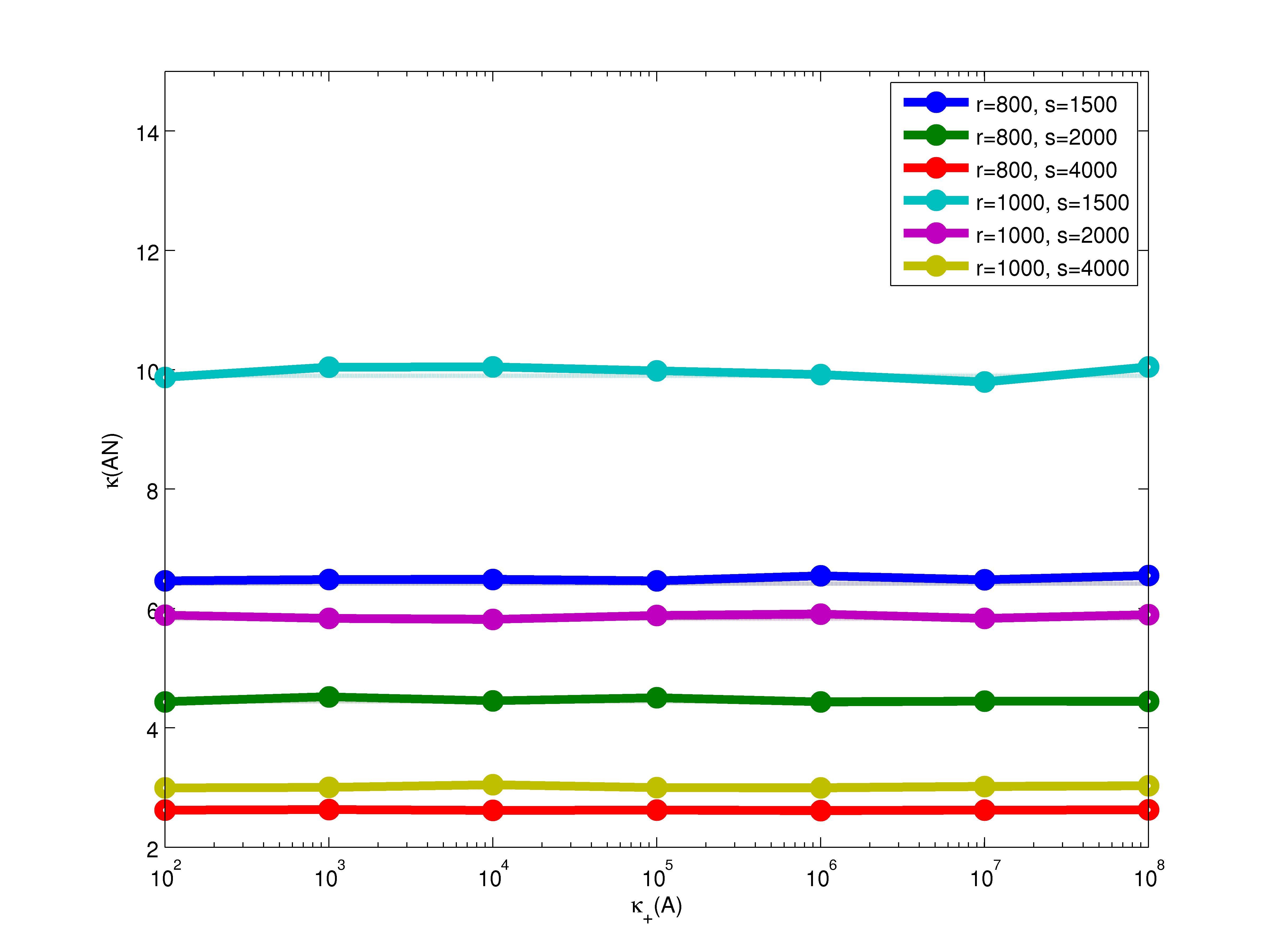
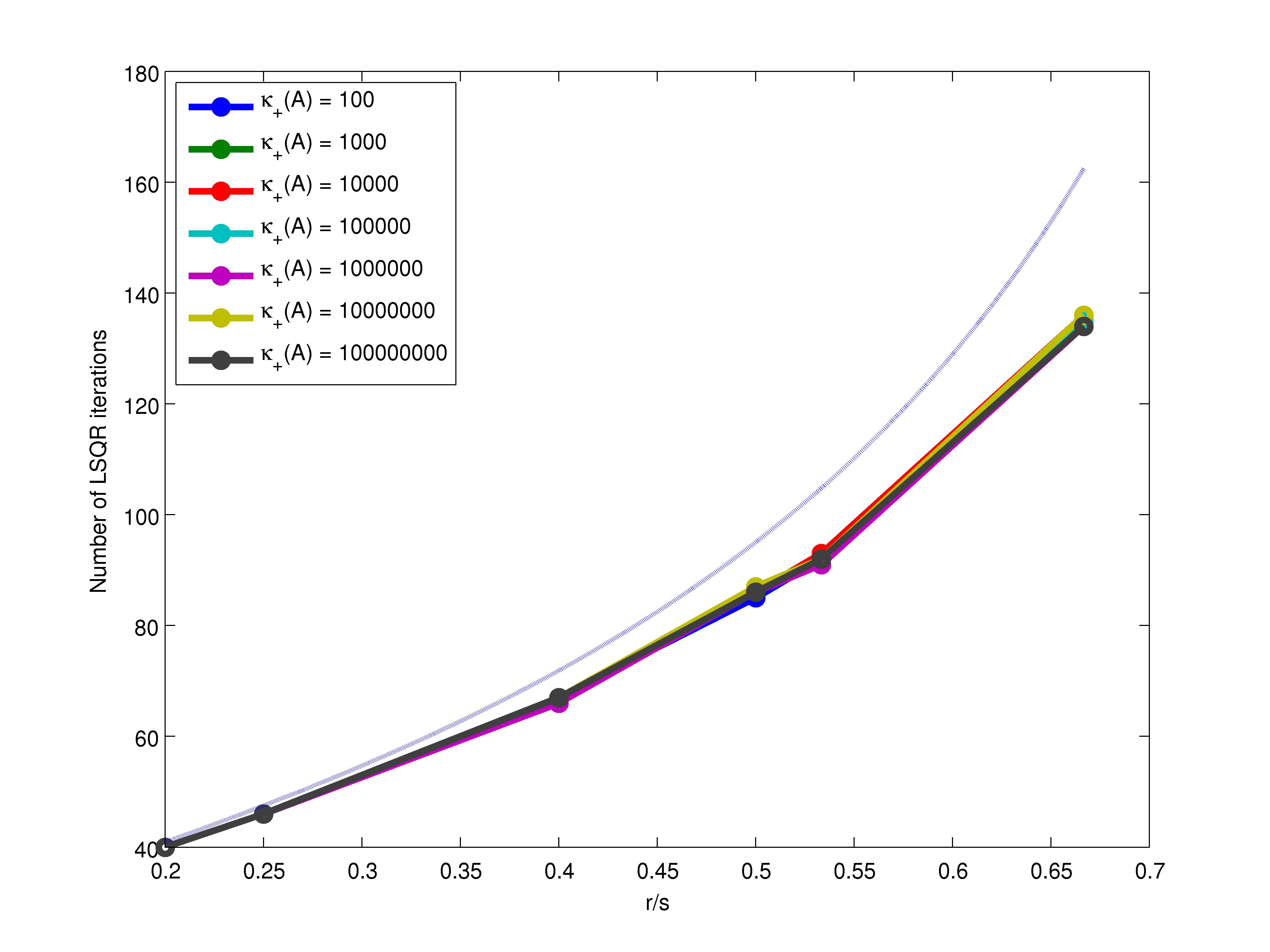
Fig. 1: Left: $\kappa_{+}(A)$ vs. $\kappa(AN)$ for different choices of $r$ and $s$. $A\in\mathbb{R}^{10^{4}\times 10^{3}}$ is randomly generated with rank $r$. For each $(r,s)$ pair, we take the largest value of $\kappa(AN)$ in 10 independent runs for each $\kappa_{+}(A)$ and connect them using a solid line. The estimate $(1+\sqrt{r/s})/(1-\sqrt{r/s})$ is drawn in a dotted line for each $(r,s)$ pair, if not overlapped with the corresponding solid line. Right: number of LSQR iterations vs. $r/s$. The number of LSQR iterations is merely a function of $r/s$, independent of the condition number of the original system.

Based on Theorem 7, the number of iterations should be less than $(\log\varepsilon-\log 2)/\log\sqrt{r/s}$, where $\varepsilon$ is a given tolerance. In order to match the accuracy of direct solvers, we set $\varepsilon=10^{-14}$. The right figure in Figure 1 shows the number of LSQR iterations for different combinations of $r/s$ and $\kappa_{+}(A)$. Again, we take the largest iteration number in $10$ independent runs for each pair of $r/s$ and $\kappa_{+}(A)$. We also draw the theoretical upper bound $(\log\varepsilon-\log 2)/\log\sqrt{r/s}$ in a dotted line. We see that the number of iterations is basically a function of $r/s$, independent of $\kappa_{+}(A)$, and the theoretical upper bound is very good in practice. This confirms that the number of iterations is fully predictable given $\gamma$.

6.3 Tuning the oversampling factor $\gamma$

Once we set the tolerance and maximum number of iterations, there is only one parameter left: the oversampling factor $\gamma$. To demonstrate the impact of $\gamma$, we fix problem size to $10^{5}\times 10^{3}$ and condition number to $10^{6}$, set the tolerance to $10^{-14}$, and then solve the problem with $\gamma$ ranged from $1.2$ to $3$. Figure 2 illustrates how $\gamma$ affects the running times of LSRN’s stages: randn for generating random numbers, mult for computing $\tilde{A}=GA$, svd for computing $\tilde{\Sigma}$ and $\tilde{V}$ from $\tilde{A}$, and iter for LSQR. We see that, the running times of randn, mult, and svd increase linearly as $\gamma$ increases, while iter time decreases. Therefore there exists an optimal choice of $\gamma$. For this particular problem, we should choose $\gamma$ between $1.8$ and $2.2$.

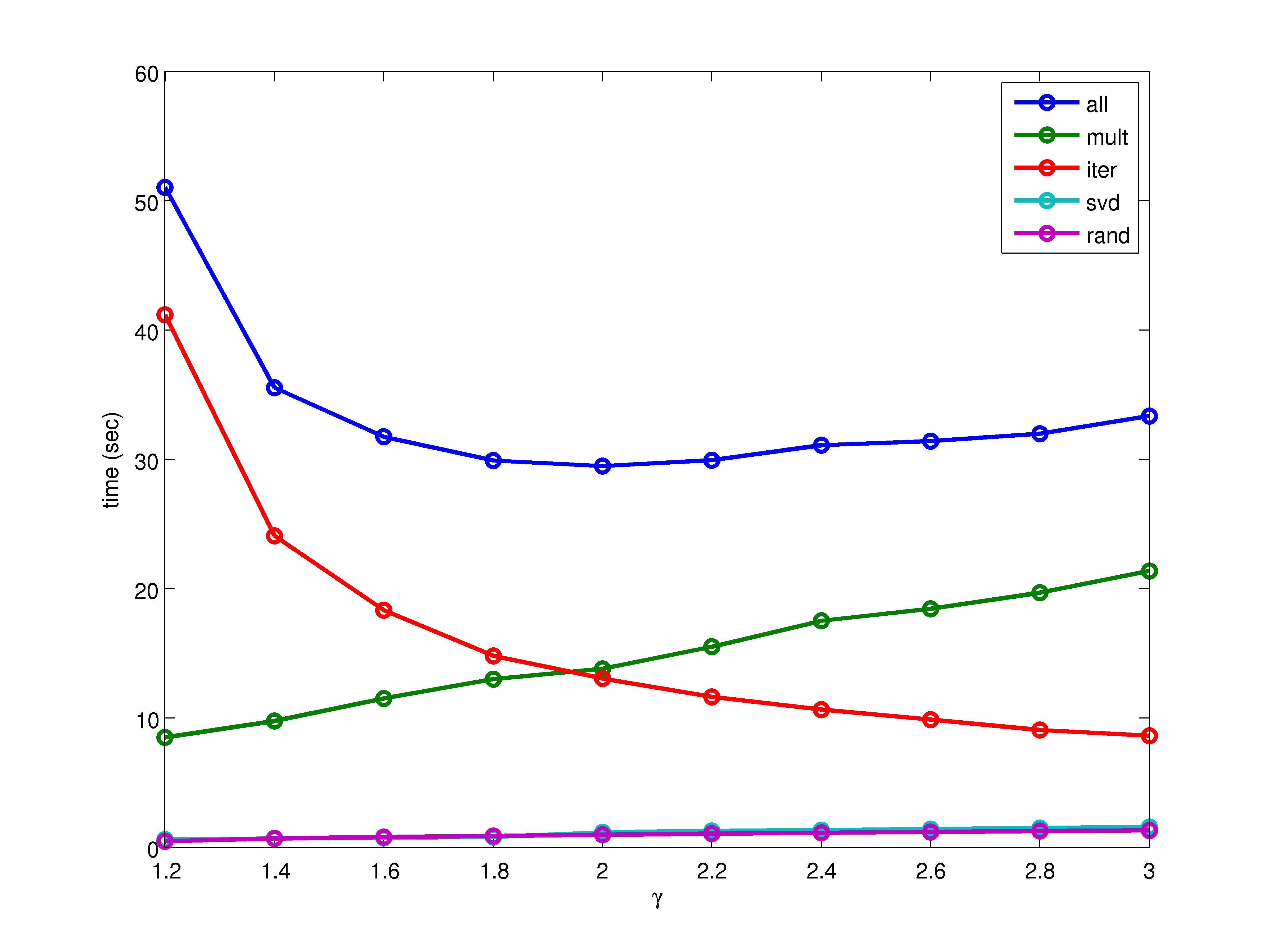
Fig. 2: The overall running time of LSRN and the running time of each LSRN stage with different oversampling factor $\gamma$ for a randomly generated problem of size $10^{5}\times 10^{3}$. For this particular problem, the optimal $\gamma$ that minimizes the overall running time lies in $[1.8,2.2]$.

We experimented with various LS problems. The best choice of $\gamma$ ranges from $1.6$ to $2.5$, depending on the type and the size of the problem. We also note that, when $\gamma$ is given, the running time of the iteration stage is fully predictable. Thus we can initialize LSRN by measuring randn/sec and flops/sec for matrix-vector multiplication, matrix-matrix multiplication, and SVD, and then determine the best value of $\gamma$ by minimizing the total running time (12). For simplicity, we set $\gamma=2.0$ in all later experiments; although this is not the optimal setting for all cases, it is always a reasonable choice.

6.4 Dense least squares

As the state-of-the-art dense linear algebra library, LAPACK provides several routines for solving LS problems, e.g., DGELS, DGELSY, and DGELSD. DGELS uses QR factorization without pivoting, which cannot handle rank-deficient problems. DGELSY uses QR factorization with pivoting, which is more reliable than DGELS on rank-deficient problems. DGELSD uses SVD. It is the most reliable routine, and should be the most expensive as well. However, we find that DGELSD actually runs much faster than DGELSY on strongly over- or under-determined systems on the shared-memory machine. It may be because of better use of multi-threaded BLAS, but we don’t have a definitive explanation.

Figure 3 compares the running times of LSRN and competing solvers on randomly generated full-rank dense strongly over- or under-determined problems. We set the condition numbers to $10^{6}$ for all problems. Note that DGELS and DGELSD almost overlapped. The results show that Blendenpik is the winner. For small-sized problems ($m\leq 3e4$), the follow-ups are DGELS and DGELSD. When the problem size goes larger, LSRN becomes faster than DGELS/DGELSD. DGELSY is always slower than DGELS/DGELSD, but still faster than MATLAB’s backslash. The performance of LAPACK’s solvers decreases significantly for under-determined problems. We monitored CPU usage and found that they couldn’t fully use all the CPU cores, i.e., they couldn’t effectively call multi-threaded BLAS. Though still the best, the performance of Blendenpik also decreases. LSRN’s performance does not change much.

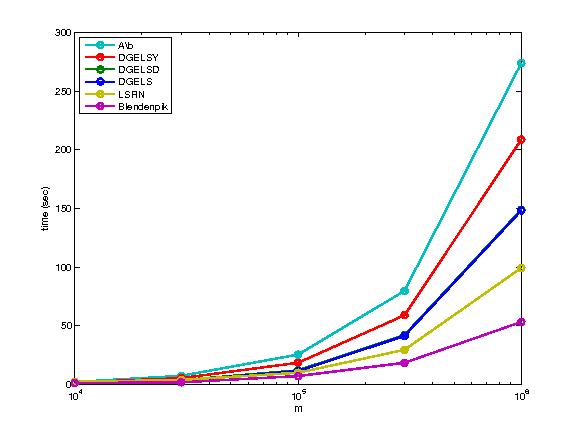
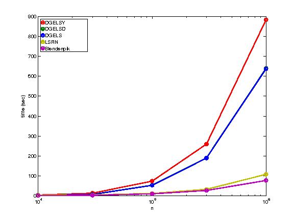
Fig. 3: Running times on $m\times 1000$ dense over-determined problems with full rank (left) and on $1000\times n$ dense under-determined problems with full rank (right). Note that DGELS and DGELSD almost overlap. When $m>3e4$, we have Blendenpik $>$ LSRN $>$ DGELS/DGELSD $>$ DGELSY $>$ $A\backslash b$ in terms of speed. On under-determined problems, LAPACK’s performance decreases significantly compared with the over-determined cases. Blendenpik’s performance decreases as well. LSRN doesn’t change much.

LSRN is also capable of solving rank-deficient problems, and in fact it takes advantage of any rank-deficiency (in that it finds a solution in fewer iterations). Figure 4 shows the results on over- and under-determined rank-deficient problems generated the same way as in previous experiments, except that we set $r=800$. DGELSY and DGELSD remain the same speed on over-determined problems as in full-rank cases, respectively, and run slightly faster on under-determined problems. LSRN’s running times reduce to $93$ seconds on the problem of size $10^{6}\times 10^{3}$, from $100$ seconds on its full-rank counterpart.

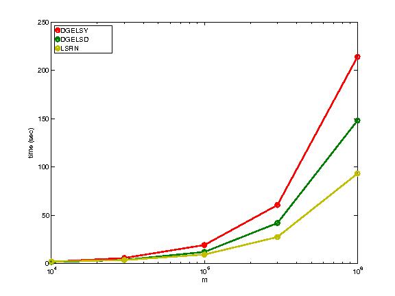
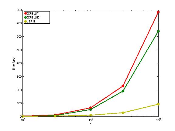
Fig. 4: Running times on $m\times 1000$ dense over-determined problems with rank $800$ (left) and on $1000\times n$ dense under-determined problems with rank $800$ (right). LSRN takes advantage of rank deficiency. We have LSRN $>$ DGSLS/DGELSD $>$ DGELSY in terms of speed.

We see that, for strongly over- or under-determined problems, DGELSD is the fastest and most reliable routine among the LS solvers provided by LAPACK. However, it (or any other LAPACK solver) runs much slower on under-determined problems than on over-determined problems, while LSRN works symmetrically on both cases. Blendenpik is the fastest dense least squares solver in our tests. Though it is not designed for solving rank-deficient problems, Blendenpik should be modifiable to handle such problems following Theorem 2. We also note that Blendenpik’s performance depends on the distribution of the row norms of $U$. We generate test problems randomly so that the row norms of $U$ are homogeneous, which is ideal for Blendenpik. When the row norms of $U$ are heterogeneous, Blendenpik’s performance may drop. See Avron, Maymounkov, and Toledo [1] for a more detailed analysis.

6.5 Sparse least squares

In LSRN, $A$ is only involved in the computation of matrix-vector and matrix-matrix multiplications. Therefore LSRN accelerates automatically when $A$ is sparse, without exploring $A$’s sparsity pattern. LAPACK does not have any direct sparse LS solver. MATLAB’s backslash uses SuiteSparseQR by Tim Davis [5] when $A$ is sparse and rectangular; this requires explicit knowledge of $A$’s sparsity pattern to obtain a sparse QR factorization.

We generated sparse LS problems using MATLAB’s “sprandn” function with density $0.01$ and condition number $10^{6}$. All problems have full rank. Figure 5 shows the results on over-determined problems. LAPACK’s solvers and Blendenpik basically perform the same as in the dense case. DGELSY is the slowest among the three. DGELS and DGELSD still overlap with each other, faster than DGELSY but slower than Blendenpik. We see that MATLAB’s backslash handles sparse problems very well. On the $10^{6}\times 10^{3}$ problem, backslash’s running time reduces to $55$ seconds, from $273$ seconds on the dense counterpart. The overall performance of MATLAB’s backslash is better than Blendenpik’s. LSRN’s curve is very flat. For small problems ($m\leq 10^{5}$), LSRN is slow. When $m>10^{5}$, LSRN becomes the fastest solver among the six. LSRN takes only $23$ seconds on the over-determined problem of size $10^{6}\times 10^{3}$. On large under-determined problems, LSRN still leads by a huge margin.

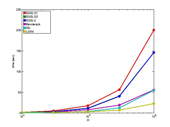
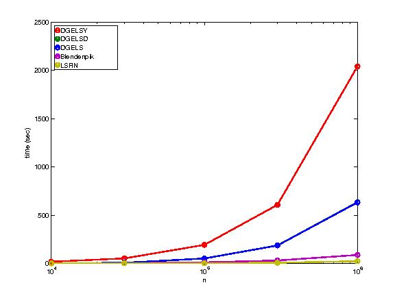
Fig. 5: Running times on $m\times 1000$ sparse over-determined problems with full rank (left) and on $1000\times n$ sparse under-determined problems with full rank (right). DGELS and DGELSD overlap with each other. LAPACK’s solvers and Blendenpik perform almost the same as in the dense case. Matlab’s backslash speeds up on sparse problems, and performs a little better than Blendenpik, but it is still slower than LSRN. LSRN leads by a huge margin on under-determined problems as well.

LSRN makes no distinction between dense and sparse problems. The speedup on sparse problems is due to faster matrix-vector and matrix-matrix multiplications. Hence, although no test was performed, we expect a similar speedup on fast linear operators as well. Also note that, in the multi-threaded implementation of LSRN, we use a naive multi-threaded routine for sparse matrix-vector and matrix-matrix multiplications, which is far from optimized and thus leaves room for improvement.

6.6 Real-world problems

In this section, we report results on some real-world large data problems. The problems are summarized in Table 2, along with running times.

Table 2: Real-world problems and corresponding running times in seconds. DGELSD doesn’t take advantage of sparsity. Though MATLAB’s backslash (SuiteSparseQR) may not give the min-length solutions to rank-deficient or under-determined problems, we still report its running times. Blendenpik either doesn’t apply to rank-deficient problems or runs out of memory (OOM). LSRN’s running time is mainly determined by the problem size and the sparsity.

matrix	$m$	$n$	nnz	rank	cond	DGELSD	$A\backslash b\ \ \$	Blendenpik	LSRN
landmark	71952	2704	1.15e6	2671	1.0e8	29.54	0.6498∗	-	17.55
rail4284	4284	1.1e6	1.1e7	full	400.0	$>3600$	$1.203^{*}$	OOM	136.0
tnimg_1	0951	1e6	2.1e7	925	-	630.6	$1067^{*}$	-	36.02
tnimg_2	1000	2e6	4.2e7	981	-	1291	$>3600^{*}$	-	72.05
tnimg_3	1018	3e6	6.3e7	1016	-	2084	$>3600^{*}$	-	111.1
tnimg_4	1019	4e6	8.4e7	1018	-	2945	$>3600^{*}$	-	147.1
tnimg_5	1023	5e6	1.1e8	full	-	$>3600$	$>3600^{*}$	OOM	188.5

landmark and rail4284 are from the University of Florida Sparse Matrix Collection [6]. landmark originated from a rank-deficient LS problem. rail4284 has full rank and originated from a linear programming problem on Italian railways. Both matrices are very sparse and have structured patterns. MATLAB’s backslash (SuiteSparseQR) runs extremely fast on these two problems, though it doesn’t guarantee to return the min-length solution. Blendenpik is not designed to handle the rank-deficient landmark, and it unfortunately runs out of memory (OOM) on rail4284. LSRN takes 17.55 seconds on landmark and 136.0 seconds on rail4284. DGELSD is slightly slower than LSRN on landmark and much slower on rail4284.

tnimg is generated from the TinyImages collection [23], which provides $80$ million color images of size $32\times 32$. For each image, we first convert it to grayscale, compute its two-dimensional DCT, and then only keep the top $2\%$ largest coefficients in magnitude. This gives a sparse matrix of size $1024\times 8\mathrm{e}7$ where each column has $20$ or $21$ nonzero elements. Note that tnimg doesn’t have apparent structured pattern. Since the whole matrix is too big, we work on submatrices of different sizes. tnimg_$i$ is the submatrix consisting of the first $10^{6}\times i$ columns of the whole matrix for $i=1,\ldots,80$, where empty rows are removed. The running times of LSRN are approximately linear in $n$. Both DGELSD and MATLAB’s backslash are very slow on the tnimg problems. Blendenpik either doesn’t apply to the rank-deficient cases or runs OOM.

We see that, though both methods taking advantage of sparsity, MATLAB’s backslash relies heavily on the sparsity pattern, and its performance is unpredictable until the sparsity pattern is analyzed, while LSRN doesn’t rely on the sparsity pattern and always delivers predictable performance and, moreover, the min-length solution.

6.7 Scalability and choice of iterative solvers on clusters

In this section, we move to the Amazon EC2 cluster. The goals are to demonstrate that (1) LSRNscales well on clusters, and (2) the CS method is preferred to LSQR on clusters with high communication cost. The test problems are submatrices of the tnimg matrix in the previous section: tnimg_4, tnimg_10, tnimg_20, and tnimg_40, solved with $4$, $10$, $20$, and $40$ cores respectively. Each process stores a submatrix of size $1024\times 1\mathrm{e}6$. Table 3 shows the results, averaged over $5$ runs.

Table 3: Test problems on the Amazon EC2 cluster and corresponding running times in seconds. When we enlarge the problem scale by a factor of $10$ and increase the number of cores accordingly, the running time only increases by a factor of $50\%$. It shows LSRN’s good scalability. Though the CS method takes more iterations, it is faster than LSQR by saving communication cost.

solver	$N_{\text{nodes}}$	np	matrix	$m$	$n$	nnz	$N_{\text{iter}}$	$T_{\text{iter}}$	$T_{\text{total}}$
LSRN w/ CS	02	04	tnimg_4	1024	4e6	8.4e7	106	34.03	170.4
LSRN w/ LSQR							084	41.14	178.6
LSRN w/ CS	05	10	tnimg_10	1024	1e7	2.1e8	106	50.37	193.3
LSRN w/ LSQR							084	68.72	211.6
LSRN w/ CS	10	20	tnimg_20	1024	2e7	4.2e8	106	73.73	220.9
LSRN w/ LSQR							084	102.3	249.0
LSRN w/ CS	20	40	tnimg_40	1024	4e7	8.4e8	106	102.5	255.6
LSRN w/ LSQR							084	137.2	290.2

Ideally, from the complexity analysis (12), when we double $n$ and double the number of cores, the increase in running time should be a constant if the cluster is homogeneous and has perfect load balancing (which we have observed is not true on Amazon EC2). For LSRN with CS, from tnimg_10 to tnimg_20 the running time increases $27.6$ seconds, and from tnimg_20 to tnimg_40 the running time increases $34.7$ seconds. We believe the difference between the time increases is caused by the heterogeneity of the cluster, because Amazon EC2 doesn’t guarantee the connection speed among nodes. From tnimg_4 to tnimg_40, the problem scale is enlarged by a factor of $10$ while the running time only increases by a factor of $50\%$. The result still demonstrates LSRN’s good scalability. We also compare the performance of LSQR and CS as the iterative solvers in LSRN. For all problems LSQR converges in $84$ iterations and CS converges in $106$ iterations. However, LSQR is slower than CS. The communication cost saved by CS is significant on those tests. As a result, we recommend CS as the default LSRN iterative solver for cluster environments. Note that to reduce the communication cost on a cluster, we could also consider increasing $\gamma$ to reduce the number of iterations.

7 Conclusion

We developed LSRN, a parallel solver for strongly over- or under-determined, and possibly rank-deficient, systems. LSRN uses random normal projection to compute a preconditioner matrix for an iterative solver such as LSQR and the Chebyshev semi-iterative (CS) method. The preconditioning process is embarrassingly parallel and automatically speeds up on sparse matrices and fast linear operators, and on rank-deficient data. We proved that the preconditioned system is consistent and extremely well-conditioned, and derived strong bounds on the number of iterations of LSQR or the CS method, and hence on the total running time. On large dense systems, LSRN is competitive with the best existing solvers, and it runs significantly faster than competing solvers on strongly over- or under-determined sparse systems. LSRN is easy to implement using threads or MPI, and it scales well in parallel environments.

References

- [1] H. Avron, P. Maymounkov, and S. Toledo, Blendenpik: Supercharging LAPACK’s least-squares solver, SIAM J. Sci. Comput., 32 (2010), pp. 1217–1236.
- [2] E. S. Coakley, V. Rokhlin, and M. Tygert, A fast randomized algorithm for orthogonal projection, SIAM J. Sci. Comput., 33 (2011), pp. 849–868.
- [3] K. R. Davidson and S. J. Szarek, Local operator theory, random matrices and Banach spaces, in Handbook of the Geometry of Banach Spaces, vol. 1, North Holland, 2001, pp. 317–366.
- [4] T. A. Davis, Direct Methods for Sparse Linear Systems, SIAM, Philadelphia, 2006.
- [5] , Algorithm 915, SuiteSparseQR: Multifrontal multithreaded rank-revealing sparse QR factorization, ACM Trans. Math. Softw., 38 (2011).
- [6] T. A. Davis and Y. Hu, The University of Florida sparse matrix collection, ACM Trans. Math. Softw., 38 (2011).
- [7] P. Drineas, M. W. Mahoney, and S. Muthukrishnan, Sampling algorithms for regression and applications, in Proceedings of the 17th Annual ACM-SIAM Symposium on Discrete Algorithms, ACM, 2006, pp. 1127–1136.
- [8] P. Drineas, M. W. Mahoney, S. Muthukrishnan, and T. Sarlós, Faster least squares approximation, Numer. Math., 117 (2011), pp. 219–249.
- [9] D. C.-L. Fong and M. Saunders, LSMR: An iterative algorithm for sparse least-squares problems, SIAM J. Sci. Comput., 33 (2011), p. 2950.
- [10] G. H. Golub and C. F. Van Loan, Matrix Computations, Johns Hopkins Univ Press, third ed., 1996.
- [11] G. H. Golub and R. S. Varga, Chebyshev semi-iterative methods, successive over-relaxation methods, and second-order Richardson iterative methods, parts I and II, Numer. Math., 3 (1961), pp. 147–168.
- [12] M. H. Gutknecht and S. Rollin, The Chebyshev iteration revisited, Parallel Comput., 28 (2002), pp. 263–283.
- [13] N. Halko, P. G. Martinsson, and J. A. Tropp, Finding structure with randomness: Probabilistic algorithms for constructing approximate matrix decompositions, SIAM Review, 53 (2011), pp. 217–288.
- [14] G. T. Herman, A. Lent, and H. Hurwitz, A storage-efficient algorithm for finding the regularized solution of a large, inconsistent system of equations, IMA J. Appl. Math., 25 (1980), pp. 361–366.
- [15] M. R. Hestenes and E. Stiefel, Methods of conjugate gradients for solving linear systems, J. Res. Nat. Bur. Stand., 49 (1952), pp. 409–436.
- [16] D. G. Luenberger, Introduction to Linear and Nonlinear Programming, Addison-Wesley, 1973.
- [17] M. W. Mahoney, Randomized Algorithms for Matrices and Data, Foundations and Trends in Machine Learning, NOW Publishers, Boston, 2011. Also available at arXiv:1104.5557v2.
- [18] G. Marsaglia and W. W. Tsang, The ziggurat method for generating random variables, J. Stat. Softw., 5 (2000), pp. 1–7.
- [19] C. C. Paige and M. A. Saunders, Solution of sparse indefinite systems of linear equations, SIAM J. Numer. Anal., 12 (1975), pp. 617–629.
- [20] , LSQR: An algorithm for sparse linear equations and sparse least squares, ACM Trans. Math. Softw., 8 (1982), pp. 43–71.
- [21] V. Rokhlin and M. Tygert, A fast randomized algorithm for overdetermined linear least-squares regression, Proc. Natl. Acad. Sci. USA, 105 (2008), pp. 13212–13217.
- [22] T. Sarlós, Improved approximation algorithms for large matrices via random projections, in Proceedings of the 47th Annual IEEE Symposium on Foundations of Computer Science, IEEE, 2006, pp. 143–152.
- [23] A. Torralba, R. Fergus, and W. T. Freeman, 80 million tiny images: A large data set for nonparametric object and scene recognition, IEEE Trans. Pattern Anal. Mach. Intell., 30 (2008), pp. 1958–1970.