Glueball masses from ratios of path integrals

Abstract:

By generalizing our previous work on the parity symmetry, the partition function of a Yang–Mills theory is decomposed into a sum of path integrals each giving the contribution from multiplets of states with fixed quantum numbers associated to parity, charge conjugation, translations, rotations and central conjugations. Ratios of path integrals and correlation functions can then be computed with a multi-level Monte Carlo integration scheme whose numerical cost, at a fixed statistical precision and at asymptotically large times, increases power-like with the time extent of the lattice. The strategy is implemented for the SU(3) Yang–Mills theory, and a full-fledged computation of the mass and multiplicity of the lightest glueball with vacuum quantum numbers is carried out at two values of the lattice spacing (0.17 and 0.12 fm).

HIM-2011-09

1 Introduction

Very often the signal-to-noise ratio of correlation functions computed by “standard” Monte Carlo techniques decreases exponentially with the time separation of the sources [1, 2]. In spectrum computations one has thereby to find compromises between large statistical errors at large time-distances and large systematic errors, due to contaminations of excited states, at short time-separations. This is not entirely satisfactory from a theoretical point of view since a solid evidence that a single state dominates, i.e. a long exponential decay over many orders of magnitude, is usually missing.

The situation is particularly unfavorable in the case of the glueball spectrum, as the variance of two-point functions at large time-distance is dominated by the vacuum [1, 2]. An intuitive way to understand the problem starts from the observation that symmetries are usually not preserved on a single gauge configuration. No matter what quantum numbers are specified at the source and sink, all states are allowed to propagate in the time direction and the expected signal emerges in the gauge average as a result of possibly large cancellations.

In a series of papers [3, 4, 5] (see also [6, 7]) we have proposed and tested a computational strategy in which, for each configuration, only states with specified quantum numbers are allowed to propagate in the time direction. In such a setup the signal-to-noise problem can be solved by introducing a hierarchical integration scheme [8, 9]. We have implemented this “Symmetry Constrained Monte Carlo” for computing the mass and the multiplicity of the lightest glueball state in the SU(3) Yang–Mills theory. Here we briefly review the basic ingredients entering that computation, the results at a rather coarse value of the lattice spacing ($a$=0.17 fm), and we present new numerical data at an additional finer resolution ($a$=0.12 fm).

2 Lattice symmetries

We aim at computing the ratio of the partition function restricted to a sector, identified by a complete set of conserved quantum numbers, over the standard one. To this end, and to fix the notation, it is useful to list the symmetry groups of the SU(3) Yang-Mills theory on a finite periodic lattice of volume $V=T\times L^{3}$, where $T$ is its time-extent and $L$ its length in each spatial directions. We will denote by $\Gamma^{\mu}({\cal{R}}_{i})$ the matrix associated to the $i$-th element of the group in the irreducible representation $\mu$.

• Parity. The group is of order 2, and the two irreducible representations of dimension 1 are $\Gamma^{(\pm)}({\mathcal{R}}_{1})=\pm\Gamma^{(\pm)}({\mathcal{R}}_{2})=1$.

• Charge Conjugation. Again this group is of order 2, and the two irreducible representations of dimension 1 are $\Gamma^{(\pm)}({\cal{R}}_{1})=\pm\Gamma^{(\pm)}({\cal{R}}_{2})=1$.

• Translations. The group of translations is a direct product of three Abelian groups, one for each space direction. Its elements are labeled by a three dimensional vector of integers ${\bf m}=({m_{1},m_{2},m_{3}})$, with ${m_{i}}=0,\dots,L-1$, where each component identifies the elements of the group in the corresponding direction. Since it is Abelian, each element forms its own class and there are $L^{3}$ non-equivalent irreducible representations of dimension 1

  $$\Gamma^{(\bf p)}({\cal{R}}_{\bf m})=e^{i\,{\bf p\cdot m}}\;,$$ (1)

  which are labeled by momentum vectors $\displaystyle{\bf p}=\frac{2\pi}{L}\,[n_{1},n_{2},n_{3}]$, with $n_{i}=0,\dots,L-1$.

• Rotations. The octahedral group is of order 24. Its elements are listed in Appendix B of [5], where explicit expressions for the $\Gamma$ matrices and the table of characters can be found for the 5 non-equivalent irreducible representations. Those are two singlets ${\rm A}_{1}$ and ${\rm A}_{2}$, one doublet ${\rm E}$ and two triplets ${\rm T}_{1}$ and ${\rm T}_{2}$.

• Central Charge Conjugations. This symmetry is strictly related to the choice of periodic boundary conditions, and it disappears in the infinite volume limit [10]. The group is a direct product of three $Z_{3}$, one for each spatial direction. It is of order 27, and its elements are labeled by a three dimensional vector of integers ${\bf\nu}=(\nu_{1},\nu_{2},\nu_{3})$, with $\nu_{i}=0,1,2$, where each component labels the elements of the Abelian group in the corresponding direction. Since each element forms its own class, there are $27$ non-equivalent irreducible representations of dimension one

  $$\Gamma^{(\bf e)}({\cal{R}}_{\bf\nu})=e^{i\,{\bf e\cdot}{\bf\nu}}\;,$$ (2)

  which are labeled by the electric flux vectors $\displaystyle{\bf e}=\frac{2\pi}{3}\,[e_{1},e_{2},e_{3}]$, with $e_{i}=0,1,2$.

3 Symmetry constrained Monte Carlo

For a discrete group of order $g$, the projector $\hat{\rm P}_{\mu}$ onto states which transform as an irreducible representation $\mu$ can be defined as (for unexplained notation see Ref. [5])

$$\hat{\rm P}^{\mu}={{n_{\mu}}\over{g}}\sum_{i=1}^{g}\chi^{(\mu)*}({\mathcal{R}}_{i})\hat{\Gamma}({\mathcal{R}}_{i})\;,$$ (3)

where $n_{\mu}$ is the dimension of the irreducible representation, $\chi^{(\mu)}({\mathcal{R}}_{i})$ is the character of the $i$th group element in that representation, and $\hat{\Gamma}({\mathcal{R}}_{i})$ is the representation of the element in the Hilbert space. The corresponding symmetry-constrained partition function can then be expressed as

$$Z^{(\mu)}(T)={\rm Tr}\left\{\hat{\rm T}^{T}\hat{\rm P}^{\mu}\right\}\;,$$ (4)

where $\hat{\rm T}$ is the transfer matrix among gauge-invariant states. By inserting (3) in the equation above and by choosing the “coordinate” basis to express the trace, it is clear that $Z^{(\mu)}(T)$ can be written as a linear combination of partition functions of $g$ different systems with twisted boundary conditions in the time direction. The latter are chosen so that the state at time $T$ is related to the one at time $0$ by a group transformation. As shown in detail in Ref. [4], the ratio $Z^{(\mu)}(T)/Z(T)$ can be factorized as a product of similar ratios associated to thick time-slices of temporal extension $d$ and fixed boundary conditions. Explicitly, we numerically compute

$${{Z^{(\mu)}(T)}\over{Z(T)}}={{1}\over{Z(T)}}\int DU\,e^{-S[U]}\,{\rm P}_{m,d}^{(\mu)}[T,0]\;,$$ (5)

where ${\rm P}_{m,d}^{(\mu)}[T,0]$ is a product of $m=T/d$ factors, and depends on the values of the spatial links on the boundaries of the thick time-slices only. Its definition is given in Refs. [4, 5]. Finally, given the locality of the gauge theory, such a factorized quantity can be very accurately estimated through a generalization of the hierarchical integration scheme proposed in Refs. [8, 9], which in this case removes completely the exponential signal-to-noise problem [3, 4, 5]. Although we focus here on partition functions, the same approach can be applied to the computation of correlation functions. Matrix elements of operators among glueball states can again be obtained avoiding the exponential signal degradation [5].

To determine the mass of the lightest glueball state with vacuum quantum numbers, we are interested in computing the ratio $Z^{({\bf e}=0,\,{\bf p},\,{\cal C}=+)}(T)/Z(T)$, which we will shorten as $Z^{({\bf p},+)}(T)/Z(T)$. The projection onto non-zero momentum is needed to get rid of the contribution from the vacuum, which would otherwise dominate the variance and cause an exponential degradation of the signal from the glueball. By applying blindly the analysis in this section, we would need to calculate the thick time-slice ratios for each of the $L^{3}\times 27\times 2$ boundary conditions. This would make the approach extremely expensive from the computational point of view, and it would give unnecessary information if one is interested in the low momentum states only. It is possible, however, to have still an exact numerical algorithm by implementing the projectors on $p_{x}$ and ${\cal C}$ exactly, while treating those on $(p_{y},p_{z})=(0,0)$ and ${\bf e}=0$ stochastically by extracting $n$ random transformations out of the associated $L^{2}\times 27$ ones and averaging over them, see Ref. [5]. As we fix singlet quantum numbers for $p_{y},p_{z}$ and ${\bf e}$, a stochastic treatment seems a priori justified, fluctuations are proportional to the exponentially suppressed higher momentum components, or to torelon contributions, which are expected to have higher energies on these volumes. The results in the next section have been obtained by using values of $n$ between 9 and 64, a choice justified a posteriori by the moderate statistical errors obtained.

Lattice	$L$	$T$	$N_{\mathrm{conf}}$	$N_{\mathrm{lev}}$	$d$
${\rm A}_{1}$	8	4	50	2	4
${\rm A}_{2}$		5	50	2	5
${\rm A}_{3}$		6	100	2	3
${\rm A}_{4}$		8	100	2	4
${\rm A}_{5}$		12	50	3	$\left\{3,6\right\}$
${\rm B}_{3}$	10	6	50	2	3
${\rm C}_{1}$	14	10	100	2	5

Table 1: Simulation parameters: $N_{\mathrm{conf}}$ is the number of configurations, $N_{\rm lev}$ is the number of levels and $d$ is the thickness of the thick time-slice used for the various levels.

Lattice	$n_{1}$	$Z^{({\bf p},+)}/Z$	$Z^{({\bf p},+)}/Z^{({\bf 0},+)}$	$aE_{\mathrm{eff}}^{({\bf{p}},+)}$
${\rm A}_{1}$	$1$	$1.6(3)\cdot 10^{-3}$	$1.04(21)\cdot 10^{-2}$	$1.14(5)$
${\rm A}_{2}$	$1$	$1.8(4)\cdot 10^{-3}$	$2.0(5)\cdot 10^{-3}$	$1.24(5)$
${\rm A}_{3}$	$1$	$4.5(7)\cdot 10^{-4}$	$4.7(7)\cdot 10^{-4}$	$1.277(25)$
${\rm A}_{4}$	$1$	$6.6(12)\cdot 10^{-5}$	$6.6(12)\cdot 10^{-5}$	$1.203(22)$
${\rm A}_{5}$	$1$	$4.1(16)\cdot 10^{-7}$	$4.3(17)\cdot 10^{-7}$	$1.22(3)$
${\rm B}_{3}$	$1$	$1.0(3)\cdot 10^{-3}$	$1.0(3)\cdot 10^{-3}$	$1.15(5)$
	$2$	$0.94(25)\cdot 10^{-4}$	$0.92(25)\cdot 10^{-4}$	$1.55(5)$
${\rm C}_{1}$	$1$	$1.5(3)\cdot 10^{-4}$	$1.5(4)\cdot 10^{-4}$	$0.883(24)$
	$2$	$2.4(22)\cdot 10^{-5}$	$2.4(22)\cdot 10^{-5}$	-

Table 2: Results for ratios of partition functions with momenta ${\bf p}=[2\pi n_{1}/L,0,0]$. The effective energy $E_{\rm eff}^{({\bf p},+)}$ is defined as in Eq. (6).

4 Results

We have simulated the SU(3) gauge theory discretized on the lattice by the Wilson action at $\beta=6/g^{2}_{0}=5.7$, and $\beta=5.85$ which correspond to a spacing of $0.17$ fm and $0.12$ fm respectively [11]. The spatial lengths are $1.4$ and $1.7$ fm, while time extends up to $2$ fm. The simulation parameters and the results are summarized in Tables 1 and 2.

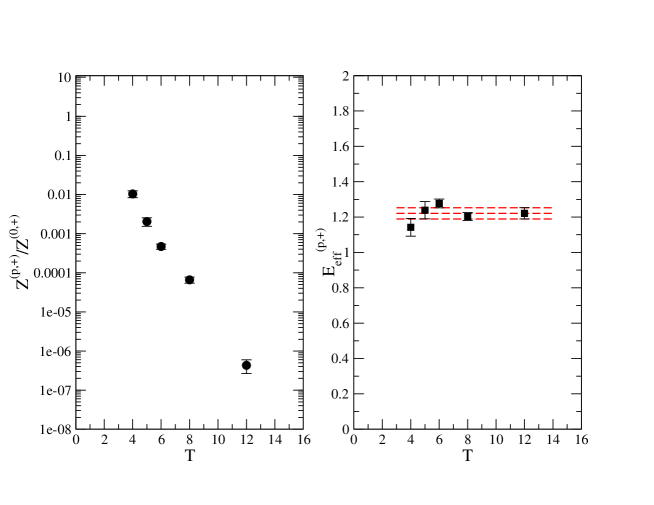
Figure 1: Left panel: ratio of partition functions $Z^{({\bf p},+)}/Z^{({\bf 0},+)}$ with momenta ${\bf p}=[2\pi/L,0,0]$ for the ${\rm A}$ lattices. Right panel: the corresponding effective energy as defined in Eq. (6). The band is our best estimate, i.e. the one extracted from the lattice with the longest time-extension.

The primary quantity that we have computed is the ratio $Z^{({\bf p},+)}/Z$ with $p_{2,3}=0$, $p_{1}=(2\pi/L)n_{1}$ and $n_{1}=1,2$. The results for the A series are shown in the left plot of Figure 1. We fit them by assuming that a single state contributes, i.e. using an ansatz of the form $\ln(Z^{({\bf p},+)}(T)/Z(T))=A-BT$, such that $A$ yields the logarithm of the multiplicity of the state and $B$ its effective, finite momentum, energy $E_{\rm eff}^{({\bf p},+)}$. At large time separations the lightest glueball with vacuum quantum numbers and momentum ${\bf p}$ is expected to dominate. The four points at the largest values of $T$ ($T/a=5,6,8,12$) in Figure 1 are well described by our ansatz, and the fit results for the multiplicity are well consistent with a value of 1 excluding 2 and 3 by three and four standard deviations respectively. We therefore define

$$E_{\rm eff}^{({\bf p},+)}=-{{1}\over{T}}\ln\left[{{Z^{({\bf p},+)}}\over{Z^{({\bf 0},+)}}}\right]\;,$$ (6)

for which the results are summarized in Table 2 and shown on the right-hand plot of Figure 1.

The lattice ${\rm B}_{3}$ serves the purpose of assessing finite size effects. It has the same lattice spacing of the ${\rm A}$ series but a linear extension of $L=10$. The results for $n_{1}=1,2$ are reported in Table 2, and are plotted as a function of the momentum squared in the left plot of Figure 2. The dashed line is a linear interpolation of the two black points (circles) of the lattice ${\rm B}_{3}$, while the red point (square) is our best result for the ${\rm A}$ series. It is rather clear that, within our statistical precision, finite volume effects are not visible in our data. It is also interesting to notice that, even if the values of the momenta are rather large, the continuum dispersion relation is well reproduced within our statistical errors. We extract the mass of the lightest glueball from the expression

$$M^{+}=\sqrt{(E_{\rm eff}^{({\bf p},+)})^{2}-{\bf p}^{2}}\;,$$ (7)

which, using the $T/a=12$ result and in units of the lattice spacing, gives

$$M^{+}=0.935\pm 0.042\;,\qquad[\beta=5.7]\;,$$ (8)

in good agreement with the estimate in Ref. [12] obtained at the same lattice spacing with the same discretization but within the standard approach. Finally, the lattice ${\rm C}_{1}$ is matched to ${\rm B}_{3}$ in volume but with a larger time extension (corresponding to $T/a=7$ at $\beta=5.7$) and more importantly with a finer lattice resolution, namely $a=0.12$ fm. By making use again of Eq. (6) to extract $E_{\rm eff}^{({\bf p},+)}$, we get from the continuum dispersion relation

$$M^{+}=0.760\pm 0.028\;,\qquad[\beta=5.85]\;,$$ (9)

in units of the lattice spacing. The results, measured in units of the scale $r_{0}$ [11], are collected in Fig. 2, where they are plotted as a function of $(a/r_{0})^{2}$ as the leading discretization effects should be quadratic in the lattice spacing.

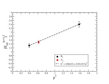
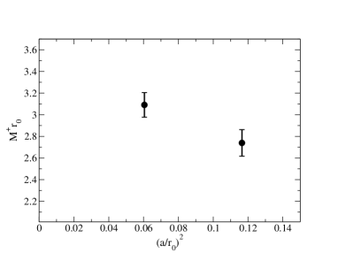
Figure 2: Left panel: the effective energy squared from the $A_{5}$ (red square) and the $B_{3}$ (black circles) lattices. Right panel: results for $r_{0}M^{+}$ at $a\simeq 0.17$ fm and $a\simeq 0.12$ fm.

5 Conclusions

We have discussed how the relative contributions to the partition function, due to states carrying a given set of quantum numbers associated with the exact symmetries of a field theory, can be expressed by ratios of path integrals with different boundary conditions in the time direction. From an algorithmic point of view, the composition properties of the projectors can be exploited to implement a hierarchical multi-level integration procedure which solves the problem of the exponential (in time) degradation of the signal-to-noise ratio.

Within this approach we have performed a precise lattice computation of the mass of the lightest glueball with vacuum quantum numbers in the SU(3) Yang-Mills theory at two values of the lattice spacing corresponding to 0.17 and 0.12 fm. The algorithm works as expected, and we have been able to follow the exponential decay up to separations of 2 fm, while keeping the error on the effective mass approximatively constant as a function of time.

Cutoff effects appear to be rather large and tend to significantly decrease the estimate of the glueball mass at finite lattice spacing, as expected and also observed in previous lattice computations [13, 14]. We are now in the process of repeating the calculation presented at a finer lattice resolution of 0.1 fm, which should eventually allow us to properly assess the magnitude of discretization effects.

The simulations were performed at CILEA, at the Swiss National Supercomputing Centre (CSCS) and at the Jülich Supercomputing Centre (JSC). We thankfully acknowledge the computer resources and technical support provided by all these institutions and their technical staff.

References

- [1] G. Parisi, Phys. Rept. 103 (1984) 203.
- [2] G.P. Lepage, TASI 89 Summer School, Boulder, CO, Jun 4-30, 1989.
- [3] M. Della Morte, L. Giusti, Comput. Phys. Commun. 180 (2009) 813.
- [4] M. Della Morte and L. Giusti, Comput. Phys. Commun. 180 (2009) 819.
- [5] M. Della Morte, L. Giusti, JHEP 1105 (2011) 056.
- [6] M. Della Morte and L. Giusti, PoS LATTICE2009 (2009) 29.
- [7] M. Della Morte, L. Giusti, PoS LATTICE2010 (2010) 250.
- [8] G. Parisi, R. Petronzio and F. Rapuano, Phys. Lett. B128 (1983) 418.
- [9] M. Lüscher and P. Weisz, JHEP 09 (2001) 010.
- [10] G. ’t Hooft, Nucl. Phys. B153 (1979) 141.
- [11] ALPHA Coll., M. Guagnelli, R. Sommer and H. Wittig, Nucl. Phys. B535 (1998) 389.
- [12] A. Vaccarino and D. Weingarten, Phys. Rev. D60 (1999) 114501.
- [13] M. Hasenbusch, S. Necco, JHEP 0408 (2004) 005.
- [14] S. Necco, Nucl.Phys. B683 (2004) 137.