The Casimir force between a microfabricated elliptic cylinder and a plate

Abstract

We investigate the Casimir force between a microfabricated elliptic cylinder (cylindrical lens) and a plate made of real materials. After a brief discussion of the fabrication procedure, which typically results in elliptic rather than circular cylinders, the Lifshitz-type formulas for the Casimir force and for its gradient are derived. In the specific case of equal semiaxes, the resulting formulas coincide with those derived previously for circular cylinders. The nanofabrication procedure may also result in asymmetric cylindrical lenses obtained from parts of two different cylinders, or rotated through some angle about the axis of the cylinder. In these cases the Lifshitz-type formulas for the Casimir force between a lens and a plate and for its gradient are also derived, and the influence of lens asymmetry is determined. Additionally, we obtain an expression for the shift of the natural frequency of a micromachined oscillator with an attached elliptic cylindrical lens interacting with a plate via the Casimir force in a nonlinear regime.

I Introduction

In recent years the Casimir effect 1 is acknowledged to be among the most rapidly developing fields of fundamental physics. It has attracted considerable attention as a test for the structure of the quantum vacuum, and for hypothetical interactions predicted in many extensions of the standard model, and also opened up new opportunities for nanotechnology 2 . Since 1997 approximately 30 experiments on measuring the Casimir force have been performed (see reviews 3 ; 4 ), which not only confirmed the currently available theoretical knowledge, but also led to unexpected results of major importance. Specifically, it was recognized 5 that the unified theory of van der Waals and Casimir forces developed by Lifshitz encounters problems in the description of free charge carriers. As a result, two theoretical approaches were proposed based on the Drude 6 ; 7 ; 8 and plasma 9 ; 10 ; 11 models. Lifshitz theory, combined with the seemingly most natural Drude model, was shown to be in contradiction with the Nernst heat theorem 2 ; 12 ; 13 ; 14 and with the experimental data 15 ; 16 . In contrast Lifshitz theory using the plasma model for the dielectric permittivity was found to be thermodynamically and experimentally consistent, despite the fact that it does not take into account the relaxation properties of free charge carriers. Note that the experiment of Refs. 15 ; 16 is an independent measurement of the gradient of the Casimir force with no fitting parameters, such as a distance offset, etc. In the first repetition of this experiment 16a measurements were performed at separations up to 1.15$\,\mu$m where zero values of the force were achieved within the limits of experimental errors. It was shown 16b that the introduction of an offset did not improve the agreement between data and the Drude model and made the agreement with the plasma model worse. Because anomalous electrostatic contributions were not observed, introducing additional parameters in the theoretical description of the experimental data was unwarranted.

This situation has been the subject of much controversy (see, for instance, Refs. 17 ; 18 ; 19 ; 20 ; 21 ). Along with the experimental and theoretical investigations mentioned above, great progress was achieved in the calculation of the Casimir force between nonplanar surfaces based on the scattering approach 2 ; 22 ; 23 ; 24 ; 25 ; 25a ; 26 . Bearing in mind, however, that in the end the elements of a scattering matrix are expressed in terms of dielectric permittivity or some other quantity characterizing material properties of the test bodies, successful application of new methods calls for the resolution of the problem of free charge carriers.

Presently great interest is expressed in new measurements of the Casimir force which could shed light on this problem. Thus, the experiment 27 claims observation of the thermal Casimir force, as predicted by the Drude model approach, in the separation region from 0.7 to $7\,\mu$m. It should be mentioned, however, that in Ref. 27 what is measured is not only the thermal Casimir force, but up to an order of magnitude greater total force presumably determined by large surface patches. The theoretical expression for the total force contains two fitting parameters determined from the best fit between the experimental data and theory. Therefore, Ref. 27 is not an independent measurement of the Casimir force as is the experiment of Refs. 15 ; 16 . In addition, it was shown 28 that the simplest version of the proximity force approximation (PFA), used in Ref. 27 to calculate both the Casimir and electric force between a spherical lens with $R=15.6\,$cm radius of curvature and a plate, is inapplicable to large lenses due to the presence of surface imperfections. Another recent experiment employing large spherical lenses 29 does not support the existence of a large thermal correction to the Casimir force predicted by the Drude model approach. Because of this, new experiments, especially exploiting more sophisticated configurations than a sphere or a spherical lens above a plate, may lead to more reliable results than those obtained in Refs. 27 ; 29 .

As a prospective alternative configuration for the measurement of the Casimir force, a cylinder-plate geometry has long been discussed in the literature 30 ; 31 ; 32 . This geometry is intermediate between the configurations of two parallel plates and a sphere above a plate. It preserves some advantages of the latter while making the problem of preserving the parallelism less difficult than for two plates. However, the configuration of cylinders with centimeter-size radii of curvature revealed anomalies in electrostatic calibrations 32 which might be caused by surface imperfections. To avoid this problem, Ref. 33 proposed an experiment measuring the thermal Casimir interaction between a plate and a microfabricated cylindrical lens attached to a micromachined oscillator. Such metallic lenses, with smooth surfaces of about $100\,\mu$m radii of curvature on top of a micromachined oscillator, can be directly fabricated by using a monolithic fabrication process. In Ref. 33 the Lifshitz-type formulas for the thermal Casimir force between a circular cylinder and a plate made of real metals were derived using the PFA. From a comparison with exact results available for ideal metals it was shown that for reasonable experimental parameters the error resulting from the use of the PFA is much less than 1%. This conclusion was confirmed in Ref. 34a for an ideal metal cylinder above an ideal metal plate. It was shown that in the region of experimental temperatures the PFA correctly reproduces the dominant contributions to both the Casimir force and thermal correction to it. The validity of the PFA was also confirmed 34b for the configuration of an atom near an ideal metal cylinder. Reference 33 demonstrated the feasibility of the proposed experiment, and investigated corrections to the Casimir force and its gradient due nonparallelity of a plate and a cylinder axis, and due to the finite length of a cylinder.

In this paper we investigate the Casimir force between a microfabricated elliptic cylinder and a plate using the PFA approach. Our consideration is adapted to the measurement scheme using a micromachined oscillator. Motivation for use of elliptic cylinders derives from the fact that fabrication procedures usually result in cylinders with semiaxes in two perpendicular directions varying by 20%–30%. Fabrication may result also in asymmetric cylindrical lenses consisting of parts of two different elliptic cylinders or rotated through some angle about the cylinder axis. In all these cases we derive the Lifshitz-type formulas for the Casimir force and for its gradient and perform computations to account for the role of asymmetry. The electric force between an elliptic cylindrical lens and a plate is also calculated for the purpose of electrostatic calibration of the Casimir setup. Furthermore, we consider an elliptic cylindrical lens attached to a micromachined oscillator and interacting with a plate via the Casimir force in the dynamic regime. We derive the exact expression for a shift of the natural frequency of the oscillator under the influence of the Casimir force. This allows measurements of the frequency shift in a nonlinear regime, and comparison of the experimental results with different theoretical approaches to the Casimir force.

The paper is organized as follows. In Sec. II the experimental procedures for microfabrication of smooth cylindrical objects are considered. In Sec. III the Lifshitz-type formulas are derived for the Casimir force and for the gradient of the Casimir force between a plate and an elliptic cylinder. In Sec. IV the same is done for an asymmetric cylindrical lens near a plate. Section V is devoted to the micromachined oscillator with an attached cylindrical lens under the influence of the Casimir force in a nonlinear regime. Section VI contains our conclusions and discussion.

II Techniques for microfabrication of smooth cylindrical objects

There are several approaches to creating a smooth cylindrical object on top of a micromachined torsional oscillator that are fully compatible with ion chromatography techniques. As a consequence, the cylindrical microstructures can be monolithically integrated with the microelectromechanical oscillators. Examples include Focused Ion Beam technology (FIB) and techniques based on femtosecond laser microfabrication.

FIB technology uses a Ga⁺ ion beam to remove material from almost any surface. The profile to be patterned can be automatically inputted and controlled rather precisely. These tools are available in almost any microfabrication laboratory and, when combined with a scanning electron microscope, they can be used for non-destructive imaging at higher magnifications, permitting extremely accurate control of the milling process T1 ; T2 . Today’s most advanced FIB tools allow direct patterning of metals with minimum contamination or damage, which opens up the possibility to directly pattern nanostructures with desirable shapes onto microelectromechanical oscillators.

Techniques based on femtosecond laser microfabrication, similar to the ones used to fabricate microlenses on glass T3 , can be also used to integrate a cylinder onto the paddle of a microelectromechanical system. In this case a tightly focused femtosecond laser beam is scanned inside a photosensitive material to create the required shape as precisely as possible. Once the photosensitive material is developed, the exposed volume will remain on the oscillator plate and standard etching processes can be used to transfer this shape to the plate.

These microfabrication techniques represent, in our opinion, the most versatile methods of fabricating microstructures of a desirable shape. For objects of cylindrical shape, microfabrication typically results in elliptic rather than circular cylinders. The actual shape of a microfabricated object can be measured very precisely using a noncontact optical profilometer. Microfabricated cylinders may have semiaxes in two perpendicular directions varying by 20%–30%. They might be also characterized by some asymmetry (for instance, the axis of a cylinder may be not exactly parallel to the plate of a microelectromechanical oscillator). More complex and expensive fabrication methods can also be used depending on the precision, uniformity and reproducibility required T4 ; T5 .

III The Casimir force between an elliptic cylinder and a plate within the proximity force approximation

We consider an elliptic cylindrical lens of thickness $h$ and width $2d$ obtained from an elliptic cylinder made of a material with a frequency-dependent dielectric permittivity $\varepsilon(\omega)$. Let the surface of this cylinder be described by the equation

$$\frac{x^{2}}{A^{2}}+\frac{(z-a-B)^{2}}{B^{2}}=1,$$ (1)

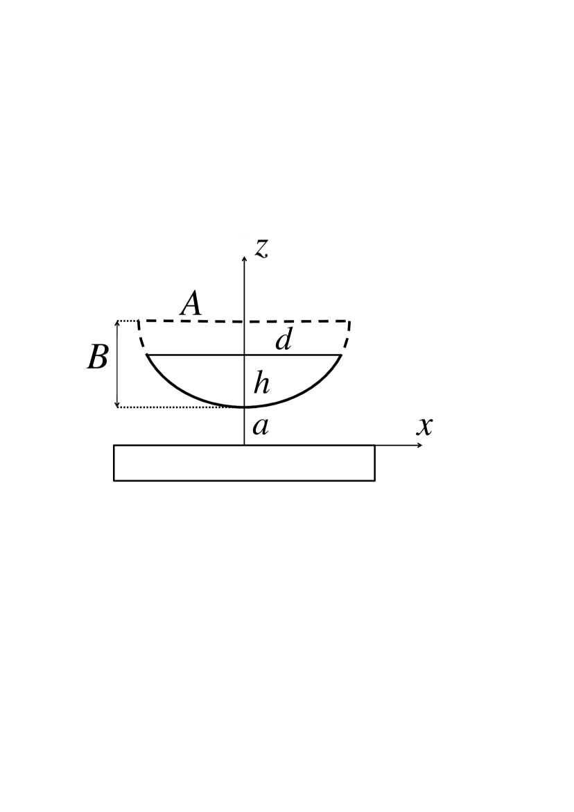
Figure 1: Elliptic cylindrical lens of thickness $h$ and width $2d$ obtained from an elliptic cylinder with semiaxes $A$ and $B$ above a plate. The figure is not to scale.

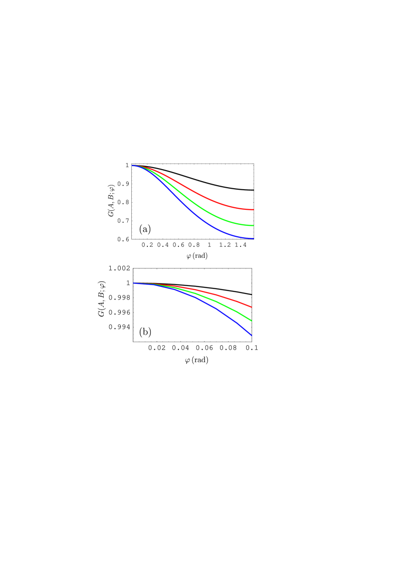
Figure 4: (Color online) The ratio of the Casimir forces between an asymmetric elliptic cylindrical lens and a plate for the angle of rotation equal to $\varphi$ and to zero as a function of $\varphi$. For different lines the ratio of cylinder semiaxes $A/B=1.1$, 1.2, 1.3, and 1.4 increasing from the top to bottom lines. The interval of the angles of rotation varies (a) from $\varphi=0$ to $\varphi=\pi/2$ and (b) from $\varphi=0$ to $\varphi=0.1\,$rad.

where $A>B$ are semiaxes and $a$ is the closest separation distance between the lens and the plate $z=0$ (see Fig. 1). The axis of a cylinder is aligned along the $y$ axis. The upper surface of a plate made of the same material coincides with the plane $z=0$. The elliptic lens under consideration is assumed to be attached to a micromachined oscillator (see Fig. 4 in Ref. 33 where a circular cylindrical lens is situated below a plate). In Fig. 1 the plate is placed below a cylindrical lens for convenience in calculations.

From Eq. (1) the explicit equation for the lens surface is given by

$$z(x)=a+B-\sqrt{B^{2}-\frac{B^{2}}{A^{2}}x^{2}}.$$ (2)

It is assumed that $a/B\ll 1$ and the lens is sufficiently thick, so that $a/h\ll 1$ as well. Applying the PFA in the general, Derjaguin, formulation 2 ; 34 to the configuration of Fig. 1 in the same way as was done in Ref. 33 for a circular cylinder, one arrives to the following Lifshitz-type formula for the Casimir force at temperature $T$:

$$F(a,T)=-\frac{2k_{B}TL}{\pi}\sum_{l=0}^{\infty}{\vphantom{\sum}}^{\!\prime}\int_{0}^{\infty}q_{l}k_{\bot}dk_{\bot}$$

$$~{}~{}~{}~{}~{}~{}~{}~{}~{}\times\sum_{n=1}^{\infty}(r_{\rm TM}^{2n}+r_{\rm TE}^{2n})\int_{0}^{d}dxe^{-2nq_{l}z(x)}.$$ (3)

Here, $k_{B}$ is the Boltzmann constant, $L$ is the length of the cylinder which is assumed to be infinitely large, $k_{\bot}$ is the projection of the wave vector on the plane $z=0$, $q_{l}=(k_{\bot}^{2}+\xi_{l}^{2}/c^{2})^{1/2}$, $\xi_{l}=2\pi k_{B}Tl/\hbar$ with $l=0,\,1,\,2,\,\ldots$ are the Matsubara frequencies, and $z(x)$ is defined in Eq. (2). The primed summation means that the term with $l=0$ is multiplied by 1/2. The reflection coefficients $r_{\rm TM}$ and $r_{\rm TE}$ for the two polarizations of the electromagnetic field (transverse magnetic and transverse electric) are given by

$$r_{\rm TM}=r_{\rm TM}(i\xi_{l},k_{\bot})=\frac{\varepsilon_{l}q_{l}-k_{l}}{\varepsilon_{l}q_{l}+k_{l}},$$

$$r_{\rm TE}=r_{\rm TE}(i\xi_{l},k_{\bot})=\frac{q_{l}-k_{l}}{q_{l}+k_{l}},$$ (4)

where $k_{l}=\left[k_{\bot}^{2}+\varepsilon_{l}{\xi_{l}^{2}}/{c^{2}}\right]^{1/2}$ and $\varepsilon_{l}=\varepsilon(i\xi_{l})$.

Bearing in mind that in accordance with Eq. (2)

$$x=x(z)=\frac{A}{B}\sqrt{B^{2}-(a+B-z)^{2}},$$ (5)

one can rearrange Eq. (3) to the form

$$F(a,T)=-\frac{2k_{B}TL}{\pi}\sum_{l=0}^{\infty}{\vphantom{\sum}}^{\!\prime}\int_{0}^{\infty}q_{l}k_{\bot}dk_{\bot}$$

$$~{}~{}~{}~{}~{}~{}~{}~{}~{}~{}\times\sum_{n=1}^{\infty}(r_{\rm TM}^{2n}+r_{\rm TE}^{2n})\int_{a}^{a+h}\!\!\!dx(z)e^{-2nq_{l}z}$$

$$=-\frac{2k_{B}TLA}{\pi B}\sum_{l=0}^{\infty}{\vphantom{\sum}}^{\!\prime}\int_{0}^{\infty}q_{l}k_{\bot}dk_{\bot}$$ (6)

$$~{}~{}\times\sum_{n=1}^{\infty}(r_{\rm TM}^{2n}+r_{\rm TE}^{2n})\int_{a}^{a+h}\!\!\!\frac{(a+B-z)e^{-2nq_{l}z}}{\sqrt{B^{2}-(a+B-z)^{2}}}\,dz.$$

We next introduce dimensionless integration variables

$$v=2aq_{l},\qquad t=nv\frac{z-a}{a}$$ (7)

instead of dimensional $k_{\bot}$ and $z$, and dimensionless Matsubara frequencies $\zeta_{l}=2a\xi_{l}/c$. As a result, from Eq. (6) we arrive at the expression

$$F(a,T)=-\frac{k_{B}TLA}{4\pi a^{2}B}\sum_{l=0}^{\infty}{\vphantom{\sum}}^{\!\prime}\sum_{n=1}^{\infty}\frac{1}{n}\int_{\zeta_{l}}^{\infty}vdv(r_{\rm TM}^{2n}+r_{\rm TE}^{2n})$$

$$~{}~{}\times e^{-nv}\int_{0}^{hnv/a}\!\!\frac{1-\frac{a}{Bnv}t}{\sqrt{1-(1-\frac{a}{Bnv}t)^{2}}}\,e^{-t}dt.$$ (8)

Here, the reflection coefficients in terms of new variables are given by

$$r_{\rm TM}=r_{\rm TM}(i\zeta_{l},v)=\frac{\varepsilon_{l}v-\sqrt{v^{2}+(\varepsilon_{l}-1)\zeta_{l}^{2}}}{\varepsilon_{l}v+\sqrt{v^{2}+(\varepsilon_{l}-1)\zeta_{l}^{2}}},$$

$$r_{\rm TE}=r_{\rm TE}(i\zeta_{l},v)=\frac{v-\sqrt{v^{2}+(\varepsilon_{l}-1)\zeta_{l}^{2}}}{v+\sqrt{v^{2}+(\varepsilon_{l}-1)\zeta_{l}^{2}}},$$ (9)

where $\varepsilon_{l}=\varepsilon(ic\zeta_{l}/2a)$.

Within the application regime of the PFA we are looking for the main contribution to the expansion of Eq. (8) in terms of the small parameter $a/B\ll 1$. To do so we can restrict our consideration to the lowest expansion order in $a/B$ of the integrand with respect to $t$. We can also set the upper integration limit of this integral equal to infinity taking into account that $h\gg a$. This leads to

$$F(a,T)=-\frac{k_{B}TL}{4\pi a^{2}}\,\frac{A}{\sqrt{2aB}}\sum_{l=0}^{\infty}{\vphantom{\sum}}^{\!\prime}\sum_{n=1}^{\infty}\frac{1}{\sqrt{n}}$$ (10)

$$~{}~{}\times\int_{\zeta_{l}}^{\infty}v^{3/2}dv(r_{\rm TM}^{2n}+r_{\rm TE}^{2n})e^{-nv}\int_{0}^{\infty}\!\!\frac{e^{-t}dt}{\sqrt{t}}.$$

After calculation of an integral with respect to $t$, and summation with respect to $n$ one obtains

$$F(a,T)=-\frac{k_{B}TL}{4\sqrt{\pi}a^{2}}\,\frac{A}{\sqrt{2aB}}\sum_{l=0}^{\infty}{\vphantom{\sum}}^{\!\prime}\int_{\zeta_{l}}^{\infty}v^{3/2}dv$$

$$~{}~{}\times\left[{\rm Li}_{1/2}(r_{\rm TM}^{2}e^{-v})+{\rm Li}_{1/2}(r_{\rm TE}^{2}e^{-v})\right],$$ (11)

where ${\rm Li}_{n}(z)$ is the polylogarithm function PBM . This is the Lifshitz-type formula for the Casimir force between an elliptic cylinder or cylindrical lens and a plate. For a circular cylinder $A=B=R$, and Eq. (11) coincides with the result derived in Ref. 33 .

In the case of an elliptic cylinder and a plate made of an ideal metal, $r_{\rm TM}^{2}=r_{\rm TE}^{2}=1$. Then at zero temperature Eq. (11) results in

$$F^{\rm IM}(a,0)=-\frac{L\hbar c}{8\pi\sqrt{\pi}a^{3}}\,\frac{A}{\sqrt{2aB}}\int_{0}^{\infty}d\zeta$$

$$~{}~{}~{}~{}~{}~{}\times\int_{\zeta}^{\infty}v^{3/2}dv\sum_{n=1}^{\infty}\frac{e^{-nv}}{\sqrt{n}}.$$ (12)

Changing the order of integrations and calculating the integrals one obtains

$$F^{\rm IM}(a,0)=-\frac{15L\hbar c}{64\pi a^{3}}\,\frac{A}{\sqrt{2aB}}\sum_{n=1}^{\infty}\frac{1}{n^{4}}.$$ (13)

After calculating the sum, the result is

$$F^{\rm IM}(a,0)=-\frac{\pi^{3}L\hbar c}{384a^{3}}\,\frac{A}{\sqrt{2aB}}.$$ (14)

For a circular cylinder ($A=B=R$) this leads to a well known result obtained in Ref. 30 .

Both Eqs. (11) and (14) are approximate, as they are obtained with the help of the PFA. Using the same considerations as in Ref. 33 , one can conclude that the relative error of these equations is approximately $0.3a/B$. For typical experimental parameters $B=100\,\mu$m and $a=200\,$nm the resulting error is equal to 0.06%.

The Lifshitz-type formula for the gradient of the Casimir force between an elliptic cylinder and a plate can be obtained by analogy with Eq. (11). For this purpose we differentiate Eq. (3) with respect to $a$ using Eq. (2) and arrive at

$$\frac{\partial F(a,T)}{\partial a}=\frac{4k_{B}TL}{\pi}\sum_{l=0}^{\infty}{\vphantom{\sum}}^{\!\prime}\int_{0}^{\infty}q_{l}^{2}k_{\bot}dk_{\bot}$$

$$~{}~{}~{}~{}~{}~{}~{}~{}~{}\times\sum_{n=1}^{\infty}n(r_{\rm TM}^{2n}+r_{\rm TE}^{2n})\int_{0}^{d}dxe^{-2nq_{l}z(x)}.$$ (15)

We then repeat the same transformations as were done in Eqs. (6)–(10) in application to Eq. (15) and obtain

$$\frac{\partial F(a,T)}{\partial a}=\frac{k_{B}TL}{4\sqrt{\pi}a^{3}}\,\frac{A}{\sqrt{2aB}}\sum_{l=0}^{\infty}{\vphantom{\sum}}^{\!\prime}\int_{\zeta_{l}}^{\infty}v^{5/2}dv$$

$$~{}~{}\times\left[{\rm Li}_{-1/2}(r_{\rm TM}^{2}e^{-v})+{\rm Li}_{-1/2}(r_{\rm TE}^{2}e^{-v})\right].$$ (16)

For a circular cylinder, Eq. (16) coincides with the result obtained in Ref. 33 . In the case of an ideal metal elliptic cylinder and a plate at zero temperature Eq. (16) leads to

$$\frac{\partial F^{\rm IM}(a,0)}{\partial a}=\frac{7\pi^{3}L\hbar c}{768a^{3}}\,\frac{A}{\sqrt{2aB}}.$$ (17)

The same equation is obtained by differentiation of Eq. (14) with respect to $a$.

The Lifshitz-type formulas (11) and (16) allow computations of the Casimir force and its gradient in the configuration of an elliptic cylindrical lens and a plate made of real materials. In so doing different theoretical approaches can be used, such as the Drude and plasma model approaches mentioned in Sec. I. For an Au circular cylinder above a plate computations of the relative thermal correction to the Casimir force and its gradient as a function of separation using the Drude and plasma model approaches were performed in Ref. 33 within the separation range from 150 nm to $5\,\mu$m. It was shown that when the Drude model is used the magnitude of the relative thermal corection to the Casimir force achieves its maximum value 41.6% at $a=2.55\,\mu$m. The maximum magnitude of the relative thermal correction to the gradient of the Casimir force 52% occurs at $a=3.6\,\mu$m. When the plasma model approach is used, the relative thermal correction to the Casimir force increases monotonically from 0.016% at 150 nm to 26.7% at $a=5\,\mu$m 33 . In the case of an elliptic cylinder the respective results for the relative thermal correction remain the same. This allows discrimination between the predictions of different theoretical approaches by comparing the computation results with the measurement data.

By using the PFA, one can also obtain a simple expression for the electric force between an elliptic cylinder and a plate. An electric force is used to perform calibrations in the measurements of the Casimir force. For a potential difference $(V-V_{0})$ between an elliptic cylinder and a plate ($V$ is the applied voltage and $V_{0}$ is the residual potential), the electric force calculated similar to the Casimir force is given by

$$F_{\rm el}(a)=-\frac{\pi\epsilon_{0}L}{2a}\,\frac{A}{\sqrt{2aB}}(V-V_{0})^{2},$$ (18)

where $\epsilon_{0}$ is the permittivity of the vacuum. For a circular cylinder $A=B=R$, this formula was obtained 31 from the exact expression for the electric force 35a

$$F_{\rm el}(a)=\frac{4\pi\epsilon_{0}L(V-V_{0})^{2}}{\Delta\ln^{2}\left(\frac{h-\Delta}{h+\Delta}\right)},$$ (19)

where $\Delta=\sqrt{h^{2}-R^{2}}$ and $h=R+a$. Expanding the right-hand side of Eq. (19) in powers of a small parameter $a/R$, one obtains

$$F_{\rm el}(a)=-\frac{\pi\epsilon_{0}L\sqrt{R}}{2\sqrt{2}a^{3/2}}(V-V_{0})^{2}\left(1-\frac{1}{12}\,\frac{a}{R}+\frac{17}{480}\,\frac{a^{2}}{R^{2}}\right).$$ (20)

Thus, for $a=100\,$nm and $R=100\,\mu$m the error in the electric force due to the use of the PFA is equal to only 0.008%.

IV An asymmetric cylindrical lens and a plate

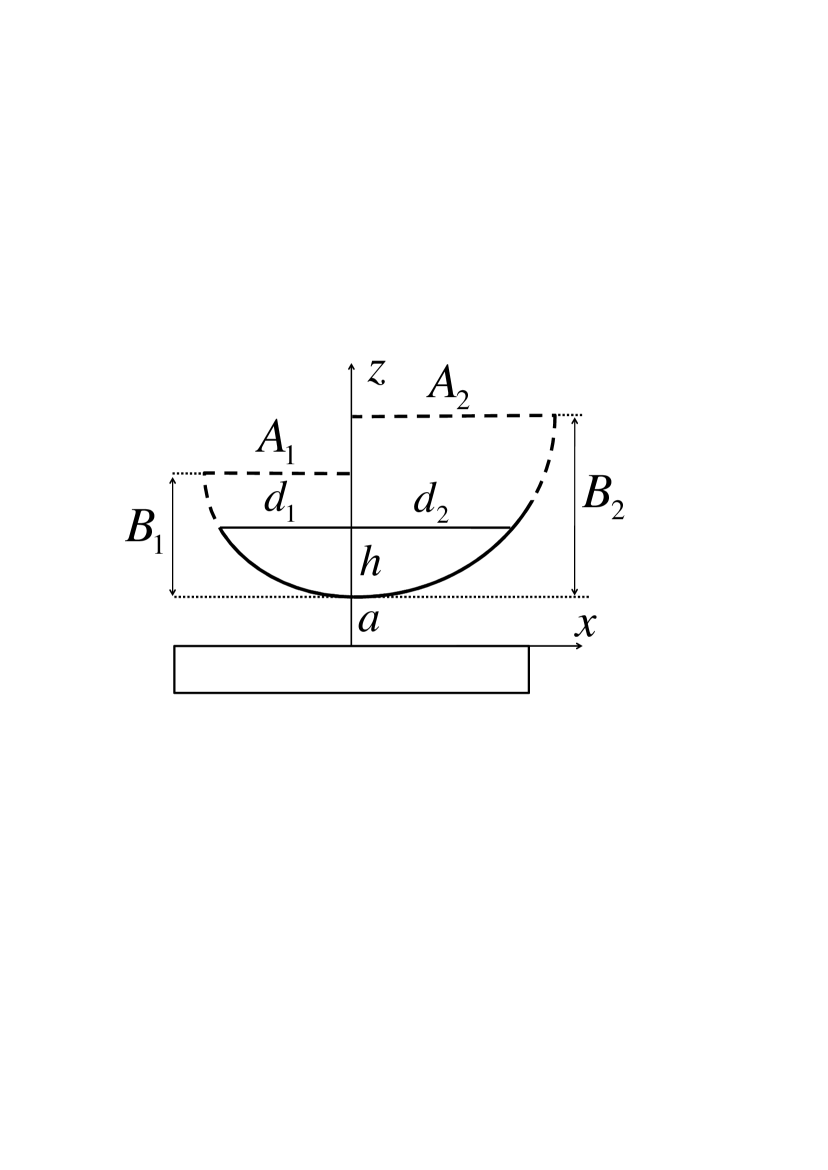
Figure 2: An asymmetric elliptic cylindrical lens of thickness $h$ and width $d_{1}+d_{2}$ obtained from two elliptic cylinders with semiaxes $A_{1},\,B_{1}$ and $A_{2},\,B_{2}$ above a plate. The figure is not to scale.

The above results can be used to calculate the Casimir force between an asymmetric cylindrical lens modeled by the two elliptic cylinders with dissimilar semiaxes $A_{1},\,B_{1}$ and $A_{2},\,B_{2}$ (see Fig. 2). One half of such a lens of width $d_{1}$ is produced as a section of an elliptic cylinder with semiaxes $A_{1},\,B_{1}$, and another half of width $d_{2}$ as a section of a cylinder with semiaxes $A_{2},\,B_{2}$. In so doing both halves are equal in thickness. Bearing in mind that the PFA is an additive method, the Casimir force between each of the halves of an asymmetric cylindrical lens and a plate can be calculated using Eq. (11). The Casimir force between the entire lens and a plate is then given by

$$F(a,T)=-\frac{k_{B}TL}{8\sqrt{\pi}a^{2}}\,\frac{1}{\sqrt{2a}}\left(\frac{A_{1}}{\sqrt{B_{1}}}+\frac{A_{2}}{\sqrt{B_{2}}}\right)$$ (21)

$$~{}~{}\times\sum_{l=0}^{\infty}{\vphantom{\sum}}^{\!\prime}\int_{\zeta_{l}}^{\infty}\!\!\!v^{3/2}dv\left[{\rm Li}_{1/2}(r_{\rm TM}^{2}e^{-v})+{\rm Li}_{1/2}(r_{\rm TE}^{2}e^{-v})\right].$$

This equation is valid under the conditions $a/B_{1}\ll 1$, $a/B_{2}\ll 1$, and $a/h\ll 1$. In a similar way, the gradient of the Casimir force between an asymmetric elliptic lens shown in Fig. 2 and a plate is expressed by the equation

$$\frac{\partial F(a,T}{\partial a})=\frac{k_{B}TL}{8\sqrt{\pi}a^{3}}\,\frac{1}{\sqrt{2a}}\left(\frac{A_{1}}{\sqrt{B_{1}}}+\frac{A_{2}}{\sqrt{B_{2}}}\right)$$ (22)

$$\times\sum_{l=0}^{\infty}{\vphantom{\sum}}^{\!\prime}\int_{\zeta_{l}}^{\infty}\!\!\!v^{5/2}dv\left[{\rm Li}_{-1/2}(r_{\rm TM}^{2}e^{-v})+{\rm Li}_{-1/2}(r_{\rm TE}^{2}e^{-v})\right].$$

Equations (21) and (22) allow calculation of the Casimir force and its gradient in the configuration of a plate and a cylindrical lens consisting of two parts of dissimilar elliptic cylinders.

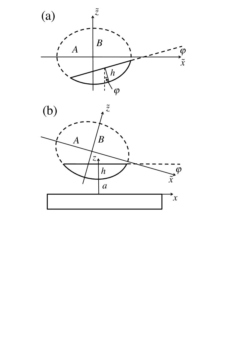
Figure 3: (a) An asymmetric elliptic cylindrical lens of thickness $h$ obtained from an elliptic cylinder with semiaxes $A$ and $B$. (b) The same asymmetric elliptic cylindrical lens spaced at the closest separation $a$ above a plate. The figure is not to scale.

We turn next to the consideration of another asymmetric cylindrical lens which is obtained from an elliptic cylinder defined in its proper coordinates ($\tilde{x},\tilde{z}$) as a cross section by the plane perpendicular to the plane $\tilde{x}\tilde{z}$ and inclined at an angle $\varphi$ to the axis $\tilde{x}$ [see Fig. 3(a)]. We then rotate the resulting lens through an angle $\varphi$ clockwise around the axis of a cylinder in order to make its base parallel to the plate [see Fig. 3(b)]. As before, the thickness of a lens is $h$.

It is easily seen that the transformation from the coordinates ($x,z$) to ($\tilde{x},\tilde{z}$) shown in Fig. 3(b) has the form

$$\tilde{x}=\tilde{x}_{0}+a\sin\varphi+x\cos\varphi-z\sin\varphi,$$

$$\tilde{z}=\tilde{z}_{0}-a\cos\varphi+x\sin\varphi+z\cos\varphi,$$ (23)

where ($\tilde{x}_{0},\tilde{z}_{0}$) are the coordinates of the lens point closest to the plate given by

$$\tilde{x}_{0}=\frac{A^{2}\sin\varphi}{H},\quad\tilde{z}_{0}=-\frac{B^{2}\cos\varphi}{H}.$$ (24)

Here, we have introduced the notation

$$H\equiv H(A,B;\varphi)=\sqrt{A^{2}\sin^{2}\varphi+B^{2}\cos^{2}\varphi}.$$ (25)

Now we substitute Eqs. (23) and (24) into the equation of a lens surface

$$\frac{\tilde{x}^{2}}{A^{2}}+\frac{\tilde{z}^{2}}{B^{2}}=1$$ (26)

written in the proper coordinates and arrive at

$$x^{2}-2x\frac{A^{2}-B^{2}}{H^{2}}(a-z)\sin\varphi\cos\varphi+2(a-z)\frac{A^{2}B^{2}}{H^{3}}$$

$$~{}~{}~{}~{}~{}~{}~{}~{}~{}+(a-z)^{2}\,\frac{A^{2}\cos^{2}\varphi+B^{2}\sin^{2}\varphi}{H^{2}}=0.$$ (27)

This equation describes the surface of an asymmetric cylindrical lens in the coordinates ($x,z$). If the inclination angle is $\varphi=0$, Eq. (27) simplifies to

$$x^{2}+2(a-z)\frac{A^{2}}{B}+(a-z)^{2}\frac{A^{2}}{B^{2}}=0,$$ (28)

and has the solution (5) as it must. For a circular cylinder $A=B=R$ and an arbitrary angle $\varphi$, Eq. (27) simplifies to

$$x^{2}+2(a-z)R+(a-z)^{2}=0,$$ (29)

leading again to the specific case of Eq. (5).

Equation (27) has the following two solutions:

$$x_{1,2}=-\frac{A^{2}-B^{2}}{H^{2}}\,(z-a)\sin\varphi\cos\varphi$$

$$~{}~{}~{}\pm\frac{AB}{H^{2}}\left[2(z-a)H-(z-a)^{2}\right]^{1/2},$$ (30)

where the upper and lower signs are for $x>0$ and $x<0$, respectively [see Fig. 3(b)].

We next consider the calculation of the thermal Casimir force between an asymmetric cylindrical lens and a plate shown in Fig. 3(b). This can be done by using the first equality in Eq. (6) which we apply separately to the parts of the lens with $x<0$ and $x>0$:

$$F_{\varphi}(a,T)=-\frac{k_{B}TL}{\pi}\sum_{l=0}^{\infty}{\vphantom{\sum}}^{\!\prime}\int_{0}^{\infty}\!\!\!q_{l}k_{\bot}dk_{\bot}\sum_{n=1}^{\infty}(r_{\rm TM}^{2n}+r_{\rm TE}^{2n})$$

$$~{}~{}~{}~{}~{}\times\left[\int_{a+h}^{a}\!\!\!dx_{2}(z)e^{-2nq_{l}z}+\int_{a}^{a+h}\!\!\!dx_{1}(z)e^{-2nq_{l}z}\right].$$ (31)

From Eq. (30), the differentials $dx_{1,2}$ are given by

$$dx_{1,2}=-\frac{(A^{2}-B^{2})\sin\varphi\cos\varphi}{H^{2}}dz$$

$$~{}~{}~{}\pm\frac{AB}{H^{2}}\frac{H-z+a}{\left[2(z-a)H-(z-a)^{2}\right]^{1/2}}dz$$ (32)

with the same sign convention as formulated above. Substituting Eq. (32) into Eq. (31), one obtains

$$F_{\varphi}(a,T)=-\frac{2k_{B}TL}{\pi}\,\frac{AB}{H^{2}}\sum_{l=0}^{\infty}{\vphantom{\sum}}^{\!\prime}\int_{0}^{\infty}\!\!\!q_{l}k_{\bot}dk_{\bot}$$ (33)

$$~{}\times\sum_{n=1}^{\infty}(r_{\rm TM}^{2n}+r_{\rm TE}^{2n})\int_{a}^{a+h}\!\!\!\frac{(H-z+a)e^{-2nq_{l}z}dz}{\left[2(z-a)H-(z-a)^{2}\right]^{1/2}}.$$

Introducing the integration variable $v$ from Eq. (7) instead of the variable $k_{\bot}$, this can be rearranged to

$$F_{\varphi}(a,T)=-\frac{k_{B}TL}{4\pi a^{3}}\,\frac{AB}{H^{2}}\sum_{l=0}^{\infty}{\vphantom{\sum}}^{\!\prime}\int_{\zeta_{l}}^{\infty}\!\!\!v^{2}dv$$ (34)

$$~{}\times\sum_{n=1}^{\infty}(r_{\rm TM}^{2n}+r_{\rm TE}^{2n})\int_{a}^{a+h}\!\!\!\frac{(H-z+a)e^{-nvz/a}dz}{\left[2(z-a)H-(z-a)^{2}\right]^{1/2}}.$$

Now, instead of the variable $z$, we introduce the variable $t$ defined in Eq. (7) and use the conditions

$$\frac{a}{h}\ll 1,\qquad\frac{a}{H}\ll 1.$$ (35)

Then Eq. (34) reduces to

$$F_{\varphi}(a,T)=-\frac{k_{B}TL}{4\sqrt{2}\pi a^{5/2}}\,\frac{AB}{H^{3/2}}\sum_{l=0}^{\infty}{\vphantom{\sum}}^{\!\prime}\int_{\zeta_{l}}^{\infty}\!\!\!v^{3/2}dv$$

$$~{}\times\sum_{n=1}^{\infty}\frac{1}{\sqrt{n}}(r_{\rm TM}^{2n}+r_{\rm TE}^{2n})e^{-nv}\int_{0}^{\infty}\!\!\!\frac{e^{t}}{\sqrt{t}}dt.$$ (36)

Performing the integration with respect to $t$ and the summation over $n$, we arrive at

$$F_{\varphi}(a,T)=-\frac{k_{B}TL}{4\sqrt{\pi}a^{2}}\,\frac{A}{\sqrt{2aB}}\left(\frac{B}{H}\right)^{3/2}\sum_{l=0}^{\infty}{\vphantom{\sum}}^{\!\prime}\int_{\zeta_{l}}^{\infty}\!\!\!v^{3/2}dv$$

$$\times\left[{\rm Li}_{1/2}(r_{\rm TM}^{2}e^{-v})+{\rm Li}_{1/2}(r_{\rm TE}^{2}e^{-v})\right].$$ (37)

The comparison of this result with Eq. (11) shows that the dependence of the Casimir force on $\varphi$ is contained exclusively in the factor

$$G(A,B;\varphi)=\left(\frac{B}{H}\right)^{3/2}\!\!\!=\left(\frac{A^{2}}{B^{2}}\sin^{2}\varphi+\cos^{2}\varphi\right)^{-{3/4}}.$$ (38)

Thus, a similar result is obtained for the gradient of the Casimir force between an asymmetric cylindrical lens and a plate

$$\frac{\partial F_{\varphi}(a,T)}{\partial a}=G(A,B;\varphi)\frac{\partial F(a,T)}{\partial a},$$ (39)

where the gradient of the Casimir force between a symmetric elliptic cylindrical lens and a plate, $\partial F(a,T)/\partial a$, is given by Eq. (16).

From Eq. (38) it is seen that the function $G$ and, thus, the Casimir force $F_{\varphi}$ and its gradient satisfy the condition

$$\frac{A}{\sqrt{B}}G\left(A,B;\varphi+\frac{\pi}{2}\right)=\frac{B}{\sqrt{A}}G(B,A;\varphi).$$ (40)

Specifically, from Eq. (40) we have

$$\frac{A}{\sqrt{B}}G\left(A,B;\frac{\pi}{2}\right)=\frac{B}{\sqrt{A}},$$ (41)

i.e., the rotation through an angle $\varphi=\pi/2$ interchanges the semiaxes of a cylinder, as it should.

In Fig. 4(a) we present the relative Casimir force and its gradient

$$\frac{F_{\varphi}(a,T)}{F(a,T)}=\frac{\partial F_{\varphi}(a,T)/\partial a}{\partial F(a,T)/\partial a}=G(A,B;\varphi)$$ (42)

as a function of the rotation angle. Different lines are for different values of the ratio of semiaxes $A/B=1.1$, 1.2, 1.3, and 1.4 increasing from the top to bottom lines. Keeping in mind that experimentally it is difficult to ensure exactly $\varphi=0$, we also present in Fig. 4(b) the same lines over a narrow interval from $\varphi=0$ to $\varphi=0.1\,$rad. From Fig. 4(a) it is seen that the relative Casimir force and its gradient decrease monotonically with the increase of $\varphi$ and $A/B$. According to Fig. 4(b), even the rotation of an elliptic lens through 0.1 rad ($5.73^{\circ}$) leads to less than 1% deviation of the Casimir force and its gradient from their respective values at $\varphi=0$ for any value of $A/B$ considered. A deviation of the Casimir force and its gradient from their values at $\varphi=0$ for less than 0.1% is achieved for the rotation angles $\varphi<0.025\,\mbox{rad}=1.43^{\circ}$. This places experimental limitations on an allowed asymmetry of the elliptic cylindrical lens used.

Note that the electric force between an asymmetric cylinder and a plate can be obtained from Eq. (18) by the replacement

$$\frac{A}{\sqrt{B}}\to\frac{1}{2}\left(\frac{A_{1}}{\sqrt{B_{1}}}+\frac{A_{2}}{\sqrt{B_{2}}}\right),$$ (43)

or by multiplying the right-hand side of Eq. (18) by the factor $G$ defined in Eq. (38) depending on the nature of asymmetry.

V Micromachined oscillator with an attached cylindrical lens in a nonlinear regime

In Ref. 33 it was proposed to perform dynamic measurements of the Casimir interaction between a plate and a circular cylinder attached to a micromachined oscillator. The proposed experiment aims to achieve the same high experimental precision, as in the experiment of Refs. 15 ; 16 for a sphere above a plate, over a wider separation region. For this purpose, the same measures, as in Refs. 15 ; 16 would be undertaken, specifically, to reduce mechanical vibrations. At any rate, the effect of vibrations in the position at the proposed measurement frequency (a few hundred hertz) is much smaller than the uncertainty in the position due to the interferometric technique used. As a result, the impact of vibrations on the determination of the gradient of the Casimir force is smaller than the current systematic experimental error, and thus, can be neglected.

As in Refs. 15 ; 16 ; 16a ; 37 ; 38 which exploited the configuration of a sphere near a plate, Ref. 33 discussed measurements of the gradient of the Casimir force in a linear regime (the same regime was employed in dynamic measurements by means of an atomic force microscope 39 ; 40 ; 41 ; 42 ; 43 ). Here, we find the frequency shift of an oscillator, caused by the Casimir force between an elliptic cylinder and a plate, in the nonlinear regime. This allows measurements down to shorter separation distances where the micromachined oscillator behaves nonlinearly.

In the dynamic regime the separation distance between an elliptic cylinder attached to a micromachined oscillator and a plate is varied with time harmonically

$$a(t)=a+A_{z}\cos\omega_{r}t.$$ (44)

Here, $\omega_{r}$ is the resonant frequency of the oscillator under the influence of the Casimir force acting between a cylinder and a plate. The amplitude of oscillations $A_{z}$ should be sufficiently small in comparison with the separation $a$. In the presence of the Casimir force, $F(a,T)$, the frequency $\omega_{r}$ is different from the natural angular frequency of the oscillator $\omega_{0}$. Such an oscillator problem was considered in Refs. 35 ; 36 perturbatively and in Ref. 44 exactly. The exact expression for the shift of the second power of the natural frequency of an oscillator produced by the Casimir force is given by 44

$$\omega_{r}^{2}-\omega_{0}^{2}=-\frac{C\omega_{r}}{\pi A_{z}}\int_{0}^{2\pi/\omega_{r}}\!\!\!\!dt\cos(\omega_{r}t)F(a+A_{z}\cos\omega_{r}t,T).$$ (45)

Here, $C$ is a constant depending on specific parameters of the setup used. Thus, for a micromachined oscillator $C=b^{2}/I$, where $b$ and $I$ are the lever arm and the moment of inertia. Note that in Ref. 44 , where the Bose-Einstein condensate was considered as a second body, the Casimir-Polder force between individual atoms and a plate was also averaged over the condensate cloud.

In the case of an elliptic cylinder interacting with the plate the force $F$ is given by Eq. (11). Representing the polilogarithm functions in Eq. (11) as power series, and replacing the integration variable $v$ with $k_{\bot}=\sqrt{v^{2}-\zeta_{l}^{2}}/(2a)$, we rearrange this equation to the form

$$F(a,T)=-\frac{k_{B}TL}{\sqrt{\pi}}\,\frac{A}{\sqrt{B}}\sum_{l=0}^{\infty}{\vphantom{\sum}}^{\!\prime}\sum_{n=1}^{\infty}\frac{1}{\sqrt{n}}\int_{0}^{\infty}\!\!\!\!k_{\bot}dk_{\bot}\sqrt{q_{l}}$$

$$~{}~{}\times(r_{\rm TM}^{2n}+r_{\rm TE}^{2n})e^{-2aq_{l}n}.$$ (46)

Substituting Eq. (46) into Eq. (45) and introducing the new integration variable $\theta=\omega_{r}t$, we arrive at

$$\omega_{r}^{2}-\omega_{0}^{2}=\frac{C}{\pi A_{z}}\frac{k_{B}TL}{\sqrt{\pi}}\,\frac{A}{\sqrt{B}}\sum_{l=0}^{\infty}{\vphantom{\sum}}^{\!\prime}\sum_{n=1}^{\infty}\frac{1}{\sqrt{n}}\int_{0}^{\infty}\!\!\!\!k_{\bot}dk_{\bot}\sqrt{q_{l}}$$

$$~{}\times(r_{\rm TM}^{2n}+r_{\rm TE}^{2n})e^{-2aq_{l}n}\!\int_{0}^{2\pi}\!d\theta\cos\theta e^{-2nA_{z}q_{l}\cos\theta}.$$ (47)

Integrating by parts, the integral with respect to $\theta$ can be reduced to 45

$$\int_{0}^{\pi}\!\sin\theta e^{\pm z\cos\theta}d\theta=\frac{\pi}{2}\,{I}_{1}(z),$$ (48)

where ${I}_{k}(z)$ is the Bessel function of an imaginary argument. The frequency shift (47) is then expressed as

$$\omega_{r}^{2}-\omega_{0}^{2}=-\frac{2C}{A_{z}}\frac{k_{B}TL}{\sqrt{\pi}}\,\frac{A}{\sqrt{B}}\sum_{l=0}^{\infty}{\vphantom{\sum}}^{\!\prime}\sum_{n=1}^{\infty}\frac{1}{\sqrt{n}}\int_{0}^{\infty}\!\!\!\!k_{\bot}dk_{\bot}$$

$$~{}\times\sqrt{q_{l}}(r_{\rm TM}^{2n}+r_{\rm TE}^{2n})e^{-2aq_{l}n}{I}_{1}(2A_{z}q_{l}n).$$ (49)

Returning to the variable $v$, one finally obtains

$$\omega_{r}^{2}-\omega_{0}^{2}=-\frac{C}{A_{z}}\frac{k_{B}TL}{2\sqrt{\pi}a^{2}}\,\frac{A}{\sqrt{2aB}}\sum_{l=0}^{\infty}{\vphantom{\sum}}^{\!\prime}\sum_{n=1}^{\infty}\frac{1}{\sqrt{n}}$$

$$~{}\times\int_{\zeta_{l}}^{\infty}\!\!\!\!v^{3/2}dv(r_{\rm TM}^{2n}+r_{\rm TE}^{2n})e^{-nv}{I}_{1}\left(\frac{A_{z}}{a}nv\right).$$ (50)

This is the general expession for the shift of the second power of the oscillator frequency due to the Casimir force between an elliptic cylindrical lens and a plate obtained using the PFA. Equation (50) takes into account nonlinearity of the oscillator. By making the replacement (43) it can be generalized to the case of an asymmetric cylindrical lens consisting of the parts of two dissimilar elliptic cylinders. Multiplying the right-hand side of Eq. (50) by the factor $G(A,B;\varphi)$ defined in Eq. (38) one obtains the generalization of Eq. (50) for the case of elliptic cylindrical lens rotated through an angle $\varphi$ (see Sec. IV).

It is easily seen that in the linear approximation Eq. (50) leads to familiar expressions commonly used in the literature 2 ; 3 ; 15 ; 16 ; 35 ; 36 ; 37 ; 38 . In fact the linear regime of the oscillator, and the first nonlinear corrections to it considered in Ref. 36 , are obtained by using the following representation for the Bessel function 45

$$I_{1}(z)=\sum_{k=0}^{\infty}\frac{\left(\frac{z}{2}\right)^{2k+1}}{k!(k+1)!}=\frac{z}{2}+\frac{z^{3}}{16}+O(z^{5}).$$ (51)

Substituting the first term on the right-hand side of this equation into Eq. (50) and performing the summation over $n$, one finds

$$\omega_{r}^{2}-\omega_{0}^{2}=-C\frac{k_{B}TL}{4\sqrt{\pi}a^{3}}\,\frac{A}{\sqrt{2aB}}\sum_{l=0}^{\infty}{\vphantom{\sum}}^{\!\prime}\int_{\zeta_{l}}^{\infty}\!\!\!\!v^{5/2}dv$$

$$~{}\times\left[{\rm Li}_{-1/2}(r_{\rm TM}^{2}e^{-v})+{\rm Li}_{-1/2}(r_{\rm TE}^{2}e^{-v})\right].$$ (52)

We can now use the Lifshitz-type formula (16) for the gradient of the Casimir force, and arrive at 2 ; 3 ; 15 ; 16 ; 35 ; 36 ; 37 ; 38

$$\omega_{r}^{2}-\omega_{0}^{2}=-C\frac{\partial F(a,T)}{\partial a}.$$ (53)

Bearing in mind that $\omega_{r}\approx\omega_{0}$ and, thus, $\omega_{r}+\omega_{0}\approx 2\omega_{0}$, Eq. (53) is often presented in the form

$$\omega_{r}=\omega_{0}\left[1-\frac{C}{2\omega_{0}^{2}}\,\frac{\partial F(a,T)}{\partial a}\right].$$ (54)

In the linear regime, Eqs. (53) and (54) allow calculation of the frequency shift of the oscillator due to the Casimir force between a plate and an elliptic cylinder. However, beyond the linear regime, the frequency shift should be calculated using Eq. (50). This allows reliable comparison between the experimental data and theoretical results for the Casimir force.

VI Conclusions and discussion

In this paper we have investigated the Casimir force acting between a plate and a microfabricated elliptic cylindrical lens made of real materials. This problem is of topical interest from the experimental point of view. The application of available technologies discussed by us in Sec. II leads to a fabrication of elliptic cylindrical lenses on top of a micromachined oscillator, rather than just the circular cylindrical lenses considered previously in the literature. We have obtained the Lifshitz-type formulas for the Casimir force and for the gradient of the Casimir force in the configuration of an elliptic cylinder and a plate. In the framework of the PFA (which is applicable at separations much less than the smaller semiaxis of an elliptic cylinder), the results for an elliptic cylinder are obtained from the respective results for a circular cylinder by replacing the cylinder radius $R$ with $A^{2}/B$, where $A$ and $B$ are the semiaxes of an elliptic cylinder (see Sec. III).

Bearing in mind that nanotechnological fabrication procedures may lead to cylinders with deviations from perfect elliptic shape, we considered two types of such deviations. In Sec. IV we obtained the Lifshitz-type formulas for the Casimir force and for its gradient in the configuration of a plate near asymmetric elliptic cylindrical lenses. Specifically, the constraints on an admissible angle of rotation of an elliptic cylindrical lens about the cylinder axis were found, allowing sufficiently small deviations from the values of the Casimir force and its gradient computed for the case of zero rotation angle. The respective results for both perfect and asymmetric elliptic cylindrical lenses were also obtained for the electrostatic force in plate-lens configuration used for calibration purposes in experiments on measuring the Casimir force. Note also that corrections to the Casimir force and its gradient due to nonparallelity of a plate and an elliptic cylinder are approximately the same as in the case of circular cylinder considered in Ref. 33 .

For the needs of several proposed experiments on measuring the Casimir force in a cylinder-plate geometry, we have considered an oscillator with an attached elliptic cylindrical lens interacting with the plane plate both made of real materials. For dynamic measurements, when the separation distance between a lens and a plate is varied harmonically, we have found the frequency shift of an oscillator due to the Casimir force in the nonlinear regime (Sec. V). The resulting equations can be used at short separations between a lens and a plate where the commonly used linear equations are not applicable. At the same time, it is shown that in the linear approximation our result yields to the known expression.

To conclude, the proposed experiment on measuring the Casimir force between a microfabricated elliptic cylindrical lens on the top of a micromachined oscillator and a plate is of much current interest and can shed additional light on the problem of thermal Casimir force.

References

- (1) H. B. G. Casimir, Proc. K. Ned. Akad. Wet. B 51, 793 (1948).
- (2) M. Bordag, G. L. Klimchitskaya, U. Mohideen, and V. M. Mostepanenko, Advances in the Casimir Effect (Oxford University Press, Oxford, 2009).
- (3) G. L. Klimchitskaya, U. Mohideen, and V. M. Mostepanenko, Rev. Mod. Phys. 81, 1827 (2009).
- (4) G. L. Klimchitskaya, U. Mohideen, and V. M. Mostepanenko, Int. J. Mod. Phys. B 25, 171 (2011).
- (5) G. L. Klimchitskaya, J. Phys.: Conf. Series 161, 012002 (2009).
- (6) M. Boström and B. E. Sernelius, Phys. Rev. Lett. 84, 4757 (2000).
- (7) J. S. Høye, I. Brevik, J. B. Aarseth, and K. A. Milton, Phys. Rev. E 67, 056116 (2003).
- (8) I. Brevik, J. B. Aarseth, J. S. Høye, and K. A. Milton, Phys. Rev. E 71, 056101 (2005).
- (9) M. Bordag, B. Geyer, G. L. Klimchitskaya, and V. M. Mostepanenko, Phys. Rev. Lett. 85, 503 (2000).
- (10) C. Genet, A. Lambrecht, and S. Reynaud, Phys. Rev. A 62, 012110 (2000).
- (11) G. L. Klimchitskaya, U. Mohideen, and V. M. Mostepanenko, J. Phys. A: Math. Theor. 40, 339 (2007).
- (12) V. B. Bezerra, G. L. Klimchitskaya, and V. M. Mostepanenko, Phys. Rev. A 65, 052113 (2002); ibid 66, 062112 (2002).
- (13) V. B. Bezerra, G. L. Klimchitskaya, V. M. Mostepanenko, and C. Romero, Phys. Rev. A 69, 022119 (2004).
- (14) M. Bordag and I. Pirozhenko, Phys. Rev. D 81, 085023 (2010).
- (15) R. S. Decca, D. López, E. Fischbach, G. L. Klimchitskaya, D. E. Krause, and V. M. Mostepanenko, Phys. Rev. D 75, 077101 (2007).
- (16) R. S. Decca, D. López, E. Fischbach, G. L. Klimchitskaya, D. E. Krause, and V. M. Mostepanenko, Eur. Phys. J. C 51, 963 (2007).
- (17) R. S. Decca, E. Fischbach, G. L. Klimchitskaya, D. E. Krause, D. López, and V. M. Mostepanenko, Phys. Rev. D 68, 116003 (2003).
- (18) B. Geyer, G. L. Klimchitskaya, and V. M. Mostepanenko, Phys. Rev. A 82, 032513 (2010).
- (19) F. Intravaia and C. Henkel, Phys. Rev. Lett. 103, 130405 (2009).
- (20) G. Bimonte, Phys. Rev. A 79, 042107 (2009).
- (21) B. E. Sernelius, Phys. Rev. A 80, 043828 (2009).
- (22) P. R. Buenzli and Ph. A. Martin, Phys. Rev. E 77, 011114 (2008).
- (23) V. M. Mostepanenko and G. L. Klimchitskaya, Int. J. Mod. Phys, A 25, 2302 (2010).
- (24) T. Emig, R. L. Jaffe, M. Kardar, and A. Scardicchio, Phys. Rev. Lett. 96, 080403 (2006).
- (25) O. Kenneth and I. Klich, Phys. Rev. Lett. 97, 160401 (2006).
- (26) M. Bordag, Phys. Rev. D 73, 125018 (2006).
- (27) T. Emig, N. Graham, R. L. Jaffe, and M. Kardar, Phys. Rev. Lett. 99, 170403 (2007).
- (28) A. Lambrecht and V. N. Marachevsky, Phys. Rev. Lett. 101, 160403 (2008).
- (29) H.-C. Chiu, G. L. Klimchitskaya, V. N. Marachevsky, V. M. Mostepanenko, and U. Mohideen, Phys. Rev. B 81, 115417 (2010).
- (30) A. O. Sushkov, W. J. Kim, D. A. R. Dalvit, and S. K. Lamoreaux, Nature Phys. 7, 230 (2011).
- (31) V. B. Bezerra, G. L. Klimchitskaya, U. Mohideen, V. M. Mostepanenko, and C. Romero, Phys. Rev. B 83, 075417 (2011).
- (32) M. Masuda and M. Sasaki, Phys. Rev. Lett. 102, 171101 (2009).
- (33) D. A. R. Dalvit, F. C. Lombardo, F. D. Mazzitelli, and R. Onofrio, Europhys. Lett. 67, 517 (2004).
- (34) M. Brown-Hayes, D. A. R. Dalvit, F. D. Mazzitelli, W. J. Kim, and R. Onofrio, Phys. Rev. A 72, 052102 (2005).
- (35) Q. Wei, D. A. R. Dalvit, F. C. Lombardo, F. D. Mazzitelli, and R. Onofrio, Phys. Rev. A 81, 052115 (2010).
- (36) R. S. Decca, E. Fischbach, G. L. Klimchitskaya, D. E. Krause, D. López, and V. M. Mostepanenko, Phys. Rev. A 82, 052515 (2010).
- (37) L. P. Teo, Phys. Rev. D 84, 025022 (2011).
- (38) V. B. Bezerra, E. R. Bezerra de Mello, G. L. Klimchitskaya, V. M. Mostepanenko, and A. A. Saharian, Eur. Phys. J. C 71, 1614 (2011).
- (39) S. Reyntjens and R. Puers, J. Micromech. Microeng. 11, 287 (2001).
- (40) S. Matsui, Three-dimensional nanostructure fabrication by focused ion beam chemical vapor deposition, in Springer Handbook of Nanotechnology, ed. B. Bhushan (Springer, Heidelberg, 2010), p.211.
- (41) Y. Cheng, H. L. Tsai, K. Sugioka and K. Midorikawa, Appl. Phys. A 85, 11 (2006).
- (42) S. Campbell, The Science and Engineering of Microelectronic Fabrication, 2nd edn. (Oxford University Press, 2001).
- (43) S. Franssila, Introduction to Microfabrication (John Wiley & Sons, London, 2004).
- (44) B. V. Derjaguin, Kolloid. Z. 69, 155 (1934).
- (45) A. P. Prudnikov, Yu. A. Brychkov, and O. I. Marichev, Integrals and Series, Vol. 2 (Gordon and Breach, New York, 1986).
- (46) W. R. Smythe, Static and Dynamic Elictricity (McGraw-Hill, New York, 1968).
- (47) G. L. Klimchitskaya, R. S. Decca, E. Fischbach, D. E. Krause, D. López, and V. M. Mostepanenko, Int. J. Mod. Phys. A 20, 2205 (2005).
- (48) R. S. Decca, D. López, E. Fischbach, G. L. Klimchitskaya, D. E. Krause, and V. M. Mostepanenko, Ann. Phys. (N.Y.) 318, 37 (2005).
- (49) G. Jourdan, A. Lambrecht, F. Comin, and J. Chevrier, Europhys. Lett. 85, 31001 (2009).
- (50) S. de Man, K. Heeck, R. J. Wijngaarden, and D. Iannuzzi, Phys. Rev. Lett. 103, 040402 (2009).
- (51) S. de Man, K. Heeck, and D. Iannuzzi, Phys. Rev. A 82, 062512 (2010).
- (52) G. Torricelli, P. J. van Zwol, O. Shpak, C. Binns, G. Palasantzas, B. J. Kooi, V. B. Svetovoy, and M. Wuttig, Phys. Rev. A 82, 010101(R) (2010).
- (53) G. Torricelli, I. Pirozhenko, S. Thornton, A. Lambrecht, and C. Binns, Europhys. Lett. 93, 51001 (2011).
- (54) H. B. Chan, V. A. Aksyuk, R. N. Kleiman, D. J. Bishop, and F. Capasso, Science, 291, 1941 (2001).
- (55) H. B. Chan, V. A. Aksyuk, R. N. Kleiman, D. J. Bishop, and F. Capasso, Phys. Rev. Lett. 87, 211801 (2001).
- (56) M. Antezza, L. P. Pitaevskii, and S. Stringari, Phys. Rev. A 70, 053619 (2004).
- (57) I. S. Gradshteyn and I. M. Ryzhik, Tables of Integrals, Series, and Products (Academic Press, New York, 1980).