Impurity-induced quasiparticle interference in the parent compounds of iron-pnictide superconductors

Abstract

The impurity-induced quasiparticle interference(QPI) in the parent compounds of iron-pnictide superconductors is investigated based on a phenomenological two-orbital four-band model and T-matrix method. We find the QPI is sensitive to the value of the magnetic order which may vary from one compound to another. For small value of the magnetic order, the pattern of oscillation in the local density of states (LDOS) induced by the QPI exhibits two-dimensional characteristics, consistent with the standing wave state observed in the $1111$ compound. For larger value of the magnetic order, the main feature of the spatial modulation of the LDOS is the existence of one-dimensional stripe structure which is in agreement with the nematic structure in the parent compound of the $122$ system. In both cases the system shows $C_{2}$ symmetry and only in the larger magnetic order case, there exist in-gap bound states. The corresponding QPI in $q$-space is also presented. The patterns of modulation in the LDOS at nonzero energies are attributed to the interplay between the underlying band structure and Fermi surfaces.

I introduction

One of the intriguing issues in condensed matter physics is the recent discovery of the new families of iron-based high-T_c superconductors. 1 ; 2 ; 3 ; 4 ; 5 ; one1 Like cuprates, superconductivity arises from electron- or hole- doping of their antiferromagnetic(AFM) parent compounds. Different from cuprates whose parent compounds are Mott insulators, the parent compounds of the iron-pnictides are bad metals whose resistivity is several orders of magnitude larger than that of normal metals. When lowing the temperature, accompanied by the formation of spin-density-wave(SDW) state, two1 ; two2 ; sdw ; jun the parent compounds of $122$ ($\mathrm{AFe_{2}As_{2}}$) undergo a tetragonal to orthorhombic structural transition while for $1111$ ($\mathrm{RFeAsO_{x}F_{y}}$) the temperature for the structural transition is higher than that for the AFM transition. Neutron-Diffraction measurements neudiff1 show that the magnetic moment ($0.87\mu_{B}$) per Fe at $5\mathrm{K}$ in $\mathrm{BaFe_{2}As_{2}}$ is substantially larger than the moment ($0.36\mu_{B}$) per Fe in $\mathrm{LaFeAsO}$. 4

Experiments on $1111$ compound helmut ; changliu ; lxyang show an extra larger hole pocket around the $\Gamma$ point, different from other pnictides due to surface polarity or surface-driven electronic structure. It is believed that the SDW picture established in the $122$ compound could apply to the $1111$ compound as well. The Fermi surfaces(FSs) of the iron-pnictides have disconnected sheets, the strong nesting between the hole FSs around the $\Gamma$ point and the electron ones around the $\mathrm{M}$ point induces the SDW instability. The formation of SDW will partially gap the FSs and will have great effect on the QPI as well as other physical properties. Before unveiling the origin of superconductivity, understanding the ordered parent compound is an important task.

Scanning tunneling microscopy (STM) on pnictides has provided much useful information on the electronic properties. stm1 ; stm2 ; stm3 For underdoped $122$ compound $\mathrm{Ca(Fe_{1-x}Co)_{2}As_{2}}$, a remarkable nematic electronic structure chuang has been observed by means of spectroscopic-imaging (SI) STM, where a one-dimensional (1D) structure aligns along the crystal a-axis with antiparallel spins, and the QPI imaging disperses predominantly along the b-axis of the material. While for the parent compound of $1111$ system $\mathrm{LaOFeAs}$, there are two types of surface after cleavage. STM studies have revealed that a two-dimensional (2D) strong standing wave pattern xiaodong induced by the QPI appears in one type of surface. And the corresponding dispersions along $q_{x}$ and $q_{y}$ are similar. Diversified electronic structure states have been observed in various systems, na0 ; th whether they play a key role in the mechanism of superconductivity na1 ; na2 has triggered much attention and motivated our investigation.

Previously, based on some effective models, the QPI has been calculated by using different methods. han ; jk ; eug ; aak ; mazin ; zho2 In order to well explain the above mentioned experiments, we solve exactly the QPI patterns as well as their Fourier component based on a phenomenological model zhang which considers the asymmetry of the As atoms above and below the Fe-Fe plane. Due to the surface effect during cleavage, the heights of the As atoms above and below the Fe-Fe plane may not be equal to each other, thus this model is suitable to study the properties of the surface layers in the iron-pnictides and should be more appropriate to describe the STM experiments which are surface-sensitive. Our study will be within the framework of T-matrix method adopted by previous works. zhang ; zjx ; zhang1 ; zhang2 The most interesting result is that we can obtain 1D and 2D modulations of the LDOS by employing the same model. The value of the magnetic order has great effect on the spatial modulation of the LDOS. Small value of magnetic order leads to 2D pattern while larger magnetic order results in 1D structure. In both cases, the patterns exhibit $C_{2}$ symmetry. To the best of our knowledge, there still lack works concerning both of the interference patterns.

The paper is organized as follows. In Sec. II, we introduce the model and work out the formalism. In Sec. III, we show the property of the normal state in the presence of impurity. In Sec. IV, we study the modulation of the LDOS induced by QPI with small value of magnetic order. In Sec. V, we investigate the QPI in the case of larger value of magnetic order. Finally, we give a summary .

II model and formalism

We start with the two-orbital four-band tight-binding phenomenological model zhang which takes the $d_{xz}$ and $d_{yz}$ orbitals of Fe ions into account and each unit cell accommodates two inequivalent Fe ions. The reason we adopt this model is that such a minimal model reproduces qualitatively the evolution of the FSs observed by angle resolved photoemission spectroscopy (ARPES) experiments 14 ; 15 ; 16 ; 17 ; 19 in both the electron- and hole- doped iron-pnictides. Based on this model, the obtained phase diagram zho , dynamic spin susceptibility gao1 , Andreev bound state inside the vortex core gao2 as well as domain wall structure huang are all consistent with the ARPES arpes , neutron scattering ns and STM stm experiments. The tight-binding part of the Hamiltonian can be expressed as

$$H_{0}= -\sum_{i\tilde{\nu}j\nu\sigma}(t_{i\tilde{\nu}j\nu}c^{\dagger}_{i\tilde{\nu}\sigma}c_{j\nu\sigma}+h.c.)-t_{0}\sum_{{\bf i}\nu\sigma}c^{\dagger}_{i\nu\sigma}c_{i\nu\sigma},$$ (1)

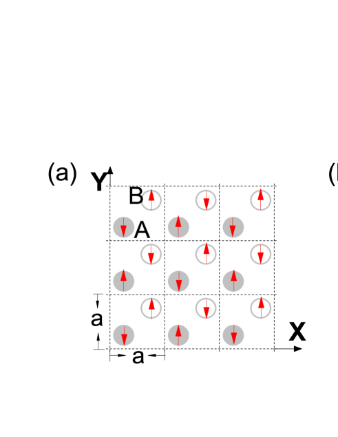
where $i,j$ are the site indices, $\tilde{\nu},\nu=0,1$ are the orbital indices, and $t_{0}$ is the chemical potential. $t_{1}$ represents the nearest-neighbor (nn) hopping between the same orbitals on Fe ions, $t_{2}$ and $t_{3}$ denote next-nearest-neighbor (nnn) hoppings between the same orbitals mediated by the up and down As ions, respectively. $t_{4}$ is the nnn hopping between different orbitals. In this paper, we adopted the hopping parameters as in Ref. zhang, , i.e. $t_{1}=0.5ev$, $t_{2}=0.4t_{1}$, $t_{3}=-2.0t_{1}$, and $t_{4}=0.04t_{1}$. In the following the energy and scattering potential are measured in unit of $t_{1}$. The distance between the nnn Fe ions is $a$ and set as unit, which is shown in Fig. 1(a).

Figure 1: (color online) (a) Schematic lattice structure of the Fe layer in the SDW state. A and B are the two inequivalent Fe ions. (b) The first Brillouin zone (red line) and the magnetic Brillouin zone (inner square). The I and III quadrants are embraced by the blue lines while the II and IV quadrants are embraced by the green ones. All the dashed lines are not included in those quadrants. The corresponding $Q_{k}$ of moving $k$ within $\mathrm{I}$ to that within $\mathrm{III}^{\prime}$ is $(-\pi,-\pi)$. In the area inside the blue (green) lines the corresponding $V_{k}=1$ $(-1)$.

With the formation of SDW, the first Brillouin zone (BZ) needs to be folded into the magnetic Brillouin zone (MBZ). The Fourier transformation of the electron destruction operator can be written as

$$c_{\mathfrak{P}i\nu\sigma} = \frac{1}{\sqrt{N}}\sum_{k}[c_{\mathfrak{P}\nu k\sigma}e^{i\textbf{k}\cdot R_{\bf{i}}}+c_{\mathfrak{P}\nu k+Q_{k}\sigma}e^{i(\textbf{k}+Q_{k})\cdot R_{\bf{i}}}]$$ (2)

$$= \frac{1}{\sqrt{N}}\sum_{k}[c^{0}_{\mathfrak{P}\nu k\sigma}e^{i\textbf{k}\cdot R_{\bf{i}}}+c^{1}_{\mathfrak{P}\nu k\sigma}e^{i(\textbf{k}+Q_{k})\cdot R_{\bf{i}}}],$$

where $N$ is the number of unit cells, $\mathfrak{P}$ can be sublattice A or B corresponding to the two inequivalent Fe ions, $k$ is restricted in the MBZ and $Q_{k}$ is chosen to be $\pm(\pi,\pi)$ or $\pm(\pi,-\pi)$, depending on which quadrant $k$ belongs to, such that $k+Q_{k}$ is in the first BZ. We have shown an example in Fig. 1(b). Here $c^{0}_{\mathfrak{P}\nu k\sigma}$ represents $c_{\mathfrak{P}\nu\sigma k}$, and $c^{1}_{\mathfrak{P}\nu k\sigma}$ represents $c_{\mathfrak{P}\nu k+Q_{k}\sigma}$. Define $C^{{\dagger}\alpha}_{\sigma}(k)=(c^{{\dagger}\alpha}_{A0k\sigma},c^{{\dagger}\alpha}_{A1k\sigma},c^{{\dagger}\alpha}_{B0k\sigma},c^{{\dagger}\alpha}_{B1k\sigma})$, then $H_{0}=\sum_{k\sigma\alpha}C^{{\dagger}\alpha}_{\sigma}M_{k}^{\alpha}C^{\alpha}_{\sigma}$, in which $\alpha=0,1$ and

$$M_{k}^{0} = \left(\begin{array}[]{cccc}a_{1}&a_{3}&a_{4}&\,0\\ a_{3}&a_{1}&\,0&a_{4}\\ a_{4}&\,0&a_{2}&a_{3}\\ \,0&a_{4}&a_{3}&a_{2}\\ \end{array}\right),$$ (7)

where $a_{1}=-2t_{2}\cos{k_{y}}-2t_{3}\cos{k_{x}}$, $a_{2}=-2t_{3}\cos{k_{y}}-2t_{2}\cos{k_{x}}$, $a_{3}=-2t_{4}(\cos{k_{x}}+\cos{k_{y}})$, $a_{4}=-2t_{1}(\cos{\frac{k_{x}+k_{y}}{2}}+\cos{\frac{k_{y}-k_{x}}{2}})$. For $M_{k}^{1}$ the corresponding $k$ changes into $k+Q_{k}$. After diagonalizing the above Hamiltonian, we obtain $H_{0}=\sum_{\mu\nu\alpha k}\epsilon^{\alpha}_{\mu\nu}(k)\psi^{{\dagger}\alpha}_{\mu\nu}(k)\psi^{\alpha}_{\mu\nu}(k)$, with the energy band indices $\alpha,\mu,\nu$ being $0$ or $1$. The analytical expressions for the eight energy bands can be written as $\epsilon^{0}_{\mu\nu}(k)=\frac{1}{2}(a_{1}+a_{2})+(-1)^{\nu}a_{3}+(-1)^{\mu}\Gamma-t_{0}$, $\epsilon^{1}_{\mu\nu}(k)=\epsilon^{0}_{\mu\nu}(k+Q_{k})$ with $\Gamma=\sqrt{\Gamma_{1}^{2}+a_{4}^{2}}$, $\Gamma_{1}=\frac{1}{2}(a_{1}-a_{2})$, and they do not depend on the spin. At half filling $t_{0}=-0.622$ and the canonical transformation matrix reads

$$\left(\begin{array}[]{c}c^{\alpha}_{A0k\sigma}\\ c^{\alpha}_{A1k\sigma}\\ c^{\alpha}_{B0k\sigma}\\ c^{\alpha}_{B1k\sigma}\\ \end{array}\right)=\left(\begin{array}[]{cccc}b^{\alpha}_{00}&-b^{\alpha}_{01}&b^{\alpha}_{10}&-b^{\alpha}_{11}\\ b^{\alpha}_{00}&\;b^{\alpha}_{01}&b^{\alpha}_{10}&\;b^{\alpha}_{11}\\ b^{\alpha}_{11}&\;b^{\alpha}_{10}&b^{\alpha}_{01}&\;b^{\alpha}_{00}\\ b^{\alpha}_{11}&-b^{\alpha}_{10}&b^{\alpha}_{01}&-b^{\alpha}_{00}\\ \end{array}\right)\left(\begin{array}[]{c}\psi^{\alpha}_{00\sigma}(k)\\ \psi^{\alpha}_{01\sigma}(k)\\ \psi^{\alpha}_{10\sigma}(k)\\ \psi^{\alpha}_{11\sigma}(k)\\ \end{array}\right).$$ (8)

The matrix elements are functions of $k$, $b^{0}_{00}=x_{1}(\Gamma+\Gamma_{1})$, $b^{0}_{01}=x_{2}a_{4}$, $b^{0}_{10}=x_{2}(\Gamma_{1}-\Gamma)$, $b^{0}_{11}=x_{1}a_{4}$ and $x_{1,2}=[2(\Gamma_{1}\pm\Gamma)^{2}+2a_{4}^{2}]^{-1/2}$ are the renormalization factors. Substituting Eq. (8) into Eq. (2), we have

$$c^{\alpha}_{A\nu k\sigma} = \sum_{\mu^{\prime},\nu^{\prime}}(-1)^{\nu^{\prime}(1-\nu)}b^{\alpha}_{\mu^{\prime}\nu^{\prime}}(k)\psi^{\alpha}_{\mu^{\prime}\nu^{\prime}\sigma}(k),$$ (9)

$$c^{\alpha}_{B\nu k\sigma} = \sum_{\mu^{\prime},\nu^{\prime}}(-1)^{\nu^{\prime}\nu}b^{\alpha}_{\mu^{\prime}+1\nu^{\prime}+1}(k)\psi^{\alpha}_{\mu^{\prime}\nu^{\prime}\sigma}(k).$$ (10)

In our coordinates, the origin is located at the A sublattice, the configuration of magnetic order is shown in Fig. 1(a). Note that magnetic order $\tilde{m}\sum_{\mu}(n_{i\mu\uparrow}-n_{i\mu\downarrow})$ varies zho with site, $\tilde{m}=me^{iQ_{k}\cdot R_{A}}$ for sublattice $A$ and $me^{iQ_{k}\cdot(R_{B}+\hat{x}/2-\hat{y}/2)}$ for sublattice $B$. The experimentally observed SDW zho term is introduced as,

$$H_{SDW} = m\;\;\sum_{\nu\alpha k\sigma}\sigma[c^{{\dagger}\alpha}_{A\nu k\sigma}c^{\alpha+1}_{A\nu k\sigma}+V_{k}c^{{\dagger}\alpha}_{B\nu k\sigma}c^{\alpha+1}_{B\nu k\sigma}],$$ (11)

$$= 2m\!\sum_{\alpha\nu\mu\mu^{\prime}k\sigma}\sigma\ B^{\alpha\mu\nu}_{\mu^{\prime}}(k)\psi^{{\dagger}\alpha}_{\mu\nu\sigma}(k)\psi^{\alpha+1}_{\mu^{\prime}\nu\sigma}(k)$$

$$B^{\alpha\mu\nu}_{\mu^{\prime}} = b^{\alpha}_{\mu\nu}b^{\alpha+1}_{\mu^{\prime}\nu}+V_{k}b^{\alpha}_{\mu+1\nu+1}b^{\alpha+1}_{\mu^{\prime}+1\nu+1},$$ (12)

$V_{k}=1$ for the first and third quadrants, otherwise $V_{k}=-1$, as shown in Fig.1(b). $\sigma$ being $\pm 1$ corresponds to spin up and spin down, respectively. A single impurity $V_{s}\sum_{\nu\sigma}c^{{\dagger}}_{A0\nu\sigma}c_{A0\nu\sigma}+V_{m}\sum_{\nu\sigma}\sigma c^{{\dagger}}_{A0\nu\sigma}c_{A0\nu\sigma}$ is located at the origin in sublattice A, the Hamiltonian of the impurity part can be written as

$$H_{imp}=\frac{2}{N}\sum_{{}^{\mu\alpha\nu\sigma k}_{\mu^{\prime}\alpha^{\prime}k^{\prime}}}(V_{s}+\sigma V_{m})b^{\alpha}_{\mu\nu}(k)b^{\alpha^{\prime}}_{\mu^{\prime}\nu}(k^{\prime})\psi^{{\dagger}\alpha}_{\mu\nu\sigma}(k)\psi^{\alpha^{\prime}}_{\mu^{\prime}\nu\sigma}(k^{\prime}),$$ (13)

where $V_{s}$ and $V_{m}$ represent the nonmagnetic part and magnetic part of the impurity potential, respectively. The total Hamiltonian is $H=H_{0}+H_{SDW}+H_{imp}$. In the following we will solve the QPI state.

Define the two-point Green’s function as

$$G^{\alpha\mu\nu\sigma}_{\alpha^{\prime}\mu^{\prime}\nu^{\prime}\sigma^{\prime}}(k,k^{\prime};i\omega_{n})=-\mathcal{F}\langle\mathrm{T}_{\tau}\psi^{\alpha}_{\mu\nu\sigma}(k,\tau)\psi^{{\dagger}\alpha^{\prime}}_{\mu^{\prime}\nu^{\prime}\sigma^{\prime}}(k^{\prime},0)\rangle,$$ (14)

where $\mathcal{F}\phi(\tau)$ denotes the Fourier transform of $\phi(\tau)$ in Matsubara frequencies, $\mathrm{T}_{\tau}$ is the time ordering operator and $\psi(\tau)=e^{\tau H}\psi e^{-\tau H}$. By using the equation of motion for Green’s function and $\frac{\partial\psi(\tau)}{\partial\tau}=e^{\tau H}[H,\psi]e^{-\tau H}$ we obtain

$$G^{\alpha\mu\nu\sigma}_{\alpha^{\prime}\mu^{\prime}\nu^{\prime}\sigma^{\prime}}(k,k^{\prime};i\omega_{n}) = mG^{0}_{\alpha\mu\nu}\sigma\!\!\!\sum_{\mu^{\prime\prime}}B^{\alpha\mu\nu}_{\mu^{\prime\prime}}(k)G^{\alpha+1\mu^{\prime\prime}\nu\sigma}_{\alpha^{\prime}\mu^{\prime}\nu^{\prime}\sigma^{\prime}}(k,k^{\prime};i\omega_{n})$$ (15)

$$+ g^{\alpha\mu\nu\sigma}_{\alpha^{\prime}\mu^{\prime}\nu^{\prime}\sigma^{\prime}}(k,k^{\prime};i\omega_{n}),$$

$$g^{\alpha\mu\nu\sigma}_{\alpha^{\prime}\mu^{\prime}\nu^{\prime}\sigma^{\prime}}(k,k^{\prime};i\omega_{n}) = G^{0}_{\alpha\mu\nu}(k,i\omega_{n})\delta_{\alpha\alpha^{\prime}}\delta_{\mu\mu^{\prime}}\delta_{\nu\nu^{\prime}}\delta_{\sigma\sigma^{\prime}}\delta_{kk^{\prime}}+$$

$$\frac{2}{N}(V_{s}\!\!+\!\sigma\!V_{m})\!\!\! G \!\!\!{}^{0}_{\alpha\mu\nu}(k,i\omega_{n})b^{\alpha}_{\mu\nu}(k)D^{\nu\sigma}_{\alpha^{\prime}\mu^{\prime}\nu^{\prime}\sigma^{\prime}}(k^{\prime},i\omega_{n}),$$ (16)

$$D^{\nu\sigma}_{\alpha^{\prime}\mu^{\prime}\nu^{\prime}\sigma^{\prime}}(k^{\prime},i\omega) = \!\!\!\sum_{\alpha^{\prime\prime}\mu^{\prime\prime}k^{\prime\prime}}\!\!b^{\alpha^{\prime\prime}}_{\mu^{\prime\prime}\nu}(k^{\prime\prime})G^{\alpha^{\prime\prime}\mu^{\prime\prime}\nu\sigma}_{\alpha^{\prime}\mu^{\prime}\nu^{\prime}\sigma^{\prime}}(k^{\prime\prime},k^{\prime};i\omega_{n}),$$ (17)

where $G^{0}_{\alpha\mu\nu}(k,i\omega_{n})=[i\omega_{n}-\epsilon^{\alpha}_{\mu\nu}(k)]^{-1}$ is the bare Green’s function. Since the translational invariance is broken by the impurity, the Green’s function depends on two momenta $k$ and $k^{\prime}$. Solving the Green’s function is the basis for calculating the LDOS, to this end, we introduce a $4\times 4$ matrix $\mathbb{S}$,

$$\begin{array}[]{c}\mathbb{S}\\ \end{array}\left(\begin{array}[]{c}G^{00\nu\sigma}_{\mu^{\prime}\nu^{\prime}\alpha^{\prime}\sigma^{\prime}}\\ G^{01\nu\sigma}_{\mu^{\prime}\nu^{\prime}\alpha^{\prime}\sigma^{\prime}}\\ G^{10\nu\sigma}_{\mu^{\prime}\nu^{\prime}\alpha^{\prime}\sigma^{\prime}}\\ G^{11\nu\sigma}_{\mu^{\prime}\nu^{\prime}\alpha^{\prime}\sigma^{\prime}}\\ \end{array}\right)=\left(\begin{array}[]{c}g^{00\nu\sigma}_{\mu^{\prime}\nu^{\prime}\alpha^{\prime}\sigma^{\prime}}\\ g^{01\nu\sigma}_{\mu^{\prime}\nu^{\prime}\alpha^{\prime}\sigma^{\prime}}\\ g^{10\nu\sigma}_{\mu^{\prime}\nu^{\prime}\alpha^{\prime}\sigma^{\prime}}\\ g^{11\nu\sigma}_{\mu^{\prime}\nu^{\prime}\alpha^{\prime}\sigma^{\prime}}\\ \end{array}\right),$$ (27)

$$\mathbb{S}=\left(\begin{array}[]{cc}I&-m\sigma S_{0}\\ -m\sigma S_{1}&I\\ \end{array}\right),$$ (30)

where $I$ is the $2\times 2$ unit matrix and

$$S_{\alpha}=\left(\begin{array}[]{cc}B^{\alpha 0\nu}_{0}G^{0}_{\alpha 0\nu}&B^{\alpha 0\nu}_{1}G^{0}_{\alpha 0\nu}\\ B^{\alpha 1\nu}_{0}G^{0}_{\alpha 1\nu}&B^{\alpha 1\nu}_{1}G^{0}_{\alpha 1\nu}\\ \end{array}\right).$$ (33)

From Eqs. (27) and (33), we finally obtain the Green’s function

$$G^{\alpha\mu\nu\sigma}_{\alpha^{\prime}\mu^{\prime}\nu^{\prime}\sigma^{\prime}}(k,k^{\prime}\!\!\! \!\!\!i\omega_{n})=\Lambda^{\alpha\mu}_{\alpha^{\prime}\mu^{\prime}}(\nu\sigma k)G^{0}_{\alpha^{\prime}\mu^{\prime}\nu}(k,i\omega_{n})\delta_{\nu\nu^{\prime}}\delta_{\sigma\sigma^{\prime}}\delta_{kk^{\prime}}$$ ; (34)

$$+ \!\frac{2}{N}(V_{s}\!+\!\sigma V_{m})D^{\nu\sigma}_{\alpha^{\prime}\mu^{\prime}\nu^{\prime}\sigma^{\prime}}(k^{\prime},i\omega_{n})f_{1}^{\alpha\mu\nu\sigma}(k),$$

$$f_{1}^{\alpha\mu\nu\sigma}(k)\! = \!\!\sum_{\alpha^{\prime\prime}\mu^{\prime\prime}}\Lambda^{\alpha\mu}_{\alpha^{\prime\prime}\mu^{\prime\prime}}(\nu\sigma k)b^{\alpha^{\prime\prime}}_{\mu^{\prime\prime}\nu}(k)G^{0}_{\alpha^{\prime\prime}\mu^{\prime\prime}\nu}(k,i\omega_{n}),$$ (35)

where $\Lambda=\mathbb{S}^{-1}$ is a matrix, the upper index $\alpha\mu$ denote the row of the elements and the lower ones denote the column of the elements. At this stage $D^{\nu\sigma}_{\alpha^{\prime}\mu^{\prime}\nu^{\prime}\sigma^{\prime}}(k^{\prime},i\omega_{n})$ is still unknown. Combining Eqs. (17) and (34), we obtain

$$D^{\nu\sigma}_{\alpha^{\prime}\mu^{\prime}}(k^{\prime},i\omega_{n}) = f_{4}^{\alpha^{\prime}\mu^{\prime}\nu^{\prime}\sigma^{\prime}}(k^{\prime})[1-2(V_{s}\!\!+\!\!\sigma V_{m})f_{2}^{\nu\sigma}]^{-1},$$ (36)

in which

$$f_{2}^{\nu\sigma} = \frac{1}{N}\sum_{\alpha\mu k}b^{\alpha}_{\mu\nu}(k)f_{1}^{\alpha\mu\nu\sigma}(k),$$ (37)

$$f_{3}^{\alpha^{\prime}\mu^{\prime}\nu\sigma}(k^{\prime}) = \sum_{\alpha\mu}\Lambda^{\alpha\mu}_{\alpha^{\prime}\mu^{\prime}}(\nu\sigma k^{\prime})b^{\alpha}_{\mu\nu}(k^{\prime}),$$ (38)

$$f_{4}^{\alpha^{\prime}\mu^{\prime}\nu^{\prime}\sigma^{\prime}}(k^{\prime}) = f_{3}^{\alpha^{\prime}\mu^{\prime}\nu\sigma}(k^{\prime})G^{0}_{\alpha^{\prime}\mu^{\prime}\nu}(k^{\prime},i\omega_{n})\delta_{\nu\nu^{\prime}}\delta_{\sigma\sigma^{\prime}}.$$ (39)

The poles of the Green’s function consist of the poles of the bare $G^{0}$ and poles of $D^{\nu\sigma}_{\alpha^{\prime}\mu^{\prime}}(k^{\prime},i\omega_{n})$, the latter ones signify the appearance of new bound states due to the impurity. From Eqs.(36)(39) we can see that the index $\nu^{\prime}\sigma^{\prime}$ of $D$ can be omitted. We also note the pole of $D^{\nu\sigma}_{\alpha^{\prime}\mu^{\prime}}(k^{\prime},i\omega_{n})$ is related to the magnitude of the magnetic order since it contains $\Lambda$. If we consider only the diagonal term of $\Lambda$, then $G^{\alpha\mu\nu\sigma}_{\alpha^{\prime}\mu^{\prime}\nu^{\prime}\sigma^{\prime}}(k,k^{\prime};i\omega_{n})=G^{0}_{\alpha\mu\nu}(k,i\omega_{n})\delta_{kk^{\prime}}+G^{0}_{\alpha\mu\nu}(k,i\omega_{n})T_{matr}G^{0}_{\alpha^{\prime}\mu^{\prime}\nu}(k^{\prime},i\omega_{n})$, which is in the form of Dyson’s equation. In real space, the LDOS of each site is $\rho(r_{i},\omega)=-\frac{1}{\pi}\Sigma_{\nu\sigma}\mathrm{Im}[-\mathcal{F}\langle T_{\tau}c_{\mathfrak{P}i\nu\sigma}(\tau)c^{{\dagger}}_{\mathfrak{P}i\nu\sigma}(0)\rangle]$. Note

$$c_{Ai\nu\sigma}(\tau)c^{{\dagger}}_{Ai\nu\sigma}(0)\!\!\! = \!\!\!\sum_{{}^{\alpha\nu k\sigma}_{\alpha^{\prime}k^{\prime}}}c^{\alpha}_{A\nu\sigma k}(\tau)c^{{\dagger}\alpha^{\prime}}_{A\nu\sigma k^{\prime}}(0)\chi^{A}_{\alpha}\chi^{A}_{\alpha^{\prime}}e^{ir_{A}\cdot(k-k^{\prime})},$$ (40)

$$c_{Bi\nu\sigma}(\tau)c^{{\dagger}}_{Bi\nu\sigma}(0)\!\!\! = \!\!\!\sum_{{}^{\alpha\nu k\sigma}_{\alpha^{\prime}k^{\prime}}}c^{\alpha}_{B\nu\sigma k}(\tau)c^{{\dagger}\alpha^{\prime}}_{B\nu\sigma k^{\prime}}(0)\chi^{A}_{\alpha}\chi^{A}_{\alpha^{\prime}}$$

$$\chi_{\alpha k}\chi_{\alpha^{\prime}k^{\prime}}e^{ir_{B}\cdot(k-k^{\prime})},$$

we derive the LDOS on sublattice $A$ and $B$ in real space, respectively. Throughout the paper we have $\chi^{A}_{\alpha}=e^{i\alpha r_{A}\cdot\tilde{q}}$, $\chi_{\alpha k}=e^{i\alpha Q_{k}\cdot r_{AB}}$, $r_{A}=(n_{1},n_{2})$, $\tilde{q}=(\pi,\pi)$, $r_{AB}=(0.5,0.5)$, and $n_{1},n_{2}$ are integers, i.e. coordinates of sites of sublattice A. The LDOS is obtained via analytic continuation $i\omega_{n}\rightarrow\omega+i\eta$ with $\eta$ being a tiny positive number and related to the lifetime of the quasiparticle. After some calculations, LDOS in real space can be expressed as follows

$$\rho(r_{A},\omega)\!\!\! = \!\!\!-\frac{2}{N\pi}\mathrm{Im}\sum_{{}^{\mu\alpha\nu\sigma k}_{\mu^{\prime}\alpha^{\prime}k^{\prime}}}[\Lambda^{\alpha\mu}_{\alpha^{\prime}\mu^{\prime}}G^{0}_{\alpha^{\prime}\mu^{\prime}\nu}(k,i\omega_{n})b^{\alpha}_{\mu\nu}(k)b^{\alpha^{\prime}}_{\mu^{\prime}\nu}(k)\chi^{A}_{\alpha}\chi^{A}_{\alpha^{\prime}}$$ (42)

$$+ \frac{2}{N}(V_{s}+\sigma V_{m})f_{1}^{\alpha\mu\nu\sigma}(k)b^{\alpha}_{\mu\nu}(k)\chi^{A}_{\alpha}$$

$$D \!\!\!{}^{\nu\sigma}_{\alpha^{\prime}\mu^{\prime}}(k^{\prime},i\omega_{n})b^{\alpha^{\prime}}_{\mu^{\prime}\nu}(k^{\prime})\chi^{A}_{\alpha^{\prime}}e^{ir_{A}\cdot(k-k^{\prime})}]|_{i\omega_{n}\rightarrow\omega+i0^{+}},$$

$$\rho(r_{B},\omega)\!\!\! = \!\!\!-\frac{2}{N\pi}\mathrm{Im}\sum_{{}^{\mu\alpha\nu\sigma k}_{\mu^{\prime}\alpha^{\prime}k^{\prime}}}[\Lambda^{\alpha\mu}_{\alpha^{\prime}\mu^{\prime}}G^{0}_{\alpha^{\prime}\mu^{\prime}\nu}(k,i\omega_{n})$$

$$b^{\alpha}_{\mu+1\nu+1}(k)b^{\alpha^{\prime}}_{\mu^{\prime}+1\nu+1}(k)\chi^{A}_{\alpha}\chi^{A}_{\alpha^{\prime}}\chi_{\alpha k}\chi_{\alpha^{\prime}k}$$

$$+ \frac{2}{N}(V_{s}+\sigma V_{m})f_{1}^{\alpha\mu\nu\sigma}(k)b^{\alpha}_{\mu+1\nu+1}(k)\chi^{A}_{\alpha}\chi_{\alpha k}$$

$$D^{\nu\sigma}_{\alpha^{\prime}\mu^{\prime}}(\!\!\!\! k \!\!\!\!{}^{\prime},i\omega_{n})b^{\alpha^{\prime}}_{\mu^{\prime}+1\nu+1}(k^{\prime})\chi^{A}_{\alpha^{\prime}}\chi_{\alpha^{\prime}k^{\prime}}e^{ir_{B}\cdot(k-k^{\prime})}]|_{i\omega_{n}\rightarrow\omega+i0^{+}}.$$ (43)

We can see that the interband scattering only exists in the same $\nu$ channel. Elastic scattering of quasiparticle mixes states having same energy but different momenta. The interference between the incoming and outgoing waves with momenta $k$ and $k^{\prime}$ can give rise to modulation of the LDOS at the wave vector $q=k-k^{\prime}$. Such kind of interference pattern can be observed in SI-STM nowadays. The Fourier component of the LDOS (FC-LDOS) can be written as,

$$\rho_{q}(\omega) = \frac{1}{2N}\sum_{r_{A}r_{B}}[\rho(r_{A},\omega)e^{iq\cdot r_{A}}+\rho(r_{B},\omega)e^{iq\cdot r_{B}}]$$

$$= -\frac{1}{2N\pi}\sum_{{}^{\alpha\nu k\sigma}_{\alpha^{\prime}k^{\prime}}}(\mathrm{Im}\{\tilde{g}_{1}(k)\}(\delta^{q}_{0}\delta^{\alpha}_{\alpha^{\prime}}+\delta^{q}_{\tilde{q}}\delta^{\alpha}_{\alpha^{\prime}+1})$$

$$+ \mathrm{Im}\{\tilde{g}_{2}(kk^{\prime})\}[\delta_{\alpha^{\prime}}^{\alpha}(\delta_{k^{\prime}}^{k+q}+\delta_{k^{\prime}}^{k-q})+\delta_{\alpha^{\prime}}^{\alpha+1}(\delta_{k^{\prime}}^{k+q+\tilde{q}}+\delta_{k^{\prime}}^{k-q+\tilde{q}})]$$

$$- i\mathrm{Re}\{\tilde{g}_{2}(kk^{\prime})\}[\delta_{\alpha^{\prime}}^{\alpha}(\delta_{k^{\prime}}^{k+q}-\delta_{k^{\prime}}^{k-q})+\delta_{\alpha^{\prime}}^{\alpha+1}(\delta_{k^{\prime}}^{k+q+\tilde{q}}-\delta_{k^{\prime}}^{k-q+\tilde{q}})]),$$

where $\tilde{g}_{1}(k)=g^{\alpha\alpha^{\prime}}_{a1}(k)+g^{\alpha\alpha^{\prime}}_{b1}(k)$, $\tilde{g}_{2}(kk^{\prime})=g^{\nu\sigma\alpha}_{a2}(k)g^{\nu\sigma\alpha^{\prime}}_{a3}(k^{\prime})+g^{\nu\sigma\alpha}_{b2}(k)g^{\nu\sigma\alpha^{\prime}}_{b3}(k^{\prime})$ and

$$g^{\alpha\alpha^{\prime}}_{a1}(k) = \sum_{\nu\mu\sigma\mu^{\prime}}\Lambda_{\alpha\mu,\alpha^{\prime}\mu^{\prime}}G^{0}_{\alpha^{\prime}\mu^{\prime}\nu}(k,i\omega_{n})b^{\alpha}_{\mu\nu}(k)b^{\alpha^{\prime}}_{\mu^{\prime}\nu}(k),$$ (45)

$$g^{\alpha\alpha^{\prime}}_{b1}(k) = \sum_{\nu\mu\sigma\mu^{\prime}}\Lambda^{\alpha\mu}_{\alpha^{\prime}\mu^{\prime}}G^{0}_{\alpha^{\prime}\mu^{\prime}\nu}(k,i\omega_{n})b^{\alpha}_{\mu\nu}(k)b^{\alpha^{\prime}}_{\mu^{\prime}+1\nu+1}(k),$$ (46)

$$g^{\nu\sigma\alpha}_{a2}(k) = \frac{2}{N}(V_{s}+\sigma V_{m})\sum_{\mu}f_{1}^{\alpha\mu\nu\sigma}(k)b^{\alpha}_{\mu\nu}(k),$$ (47)

$$g^{\nu\sigma\alpha}_{b2}(k) = \frac{2}{N}(V_{s}+\sigma V_{m})\sum_{\mu}f_{1}^{\alpha\mu\nu\sigma}(k)b^{\alpha}_{\mu+1\nu+1}(k)\chi_{\alpha k},$$ (48)

$$g^{\nu\sigma\alpha^{\prime}}_{a3}(k^{\prime}) = \sum_{\mu^{\prime}}D^{\nu\sigma}_{\alpha^{\prime}\mu^{\prime}}(k^{\prime},i\omega_{n})b^{\alpha^{\prime}}_{\mu^{\prime}\nu}(k^{\prime}),$$ (49)

$$g^{\nu\sigma\alpha^{\prime}}_{b3}(k^{\prime}) = \sum_{\mu^{\prime}}D^{\nu\sigma}_{\alpha^{\prime}\mu^{\prime}}(k^{\prime},i\omega_{n})b^{\alpha^{\prime}}_{\mu^{\prime}+1\nu+1}(k^{\prime})\chi_{\alpha^{\prime}k^{\prime}}.$$ (50)

Since the QPI in our model has $C_{2}$ symmetry, which will be seen clearly in the remaining paper, the last line of Eq.(II) will be zero, thus we only show the absolute value of the real part in the corresponding figures of FC-LDOS. The map is confined in the first BZ and we perform our calculation with $N=800\times 800$ unit cells. We neglect the component of $\tilde{g}_{1}(k)$ since we want to see the QPI induced by impurity clearly. Different from the superconducting phase in which magnetic impurity and nonmagnetic one have distinct effect on the LDOS. zhang In the SDW state our calculations show that the effect of a pure magnetic impurity ($\sigma V_{m}$) is very similar to that of a pure nonmagnetic one ($V_{s}$). While for the mixed scattering potential $V_{s}+\sigma V_{m}$, the effect of the magnetic part is similar to varying the value of magnetic order, so in the following, we consider only the QPI induced by nonmagnetic impurity with different values of magnetic order.

Figure 2: (color online) Panel (a) plots the Fermi surface of the tight-binding model in the first BZ. Panel (b) plots the LDOS of the tight-binding model. Panel (c) shows the LDOS of $m=0.2,0.6$ without the impurity. Panel (d) shows the zero temperature spectral function for $m=0.2$ in the MBZ (denoted by grey color). There are four small pockets ($P\nu_{1},P\nu_{0},P\nu^{\prime}_{0},P\nu^{\prime}_{1}$) aligning along the diagonal direction and two high-intensity squares ($L\nu_{0}$, $L\nu_{1}$). Panel (e) is similar to panel (d), but for $m=0.6$, here only four pockets are left.

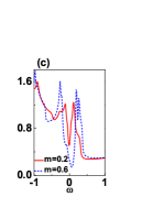
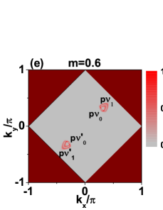
The impurity effect in the SDW state depends on the detail of electronic structure. Since we mainly focus on the low-energy structures of the LDOS, the FS topology should be important for the results. The black lines in Figs. 2(a) show the FSs of the tight-binding model, where the two hole pockets centered around $\Gamma$ point $(0,0)$ are associated with $\epsilon_{1\nu}$, and the two electron ones around $M$ point $\pi(\pm 1,\pm 1)$ are associated with $\epsilon_{0\nu}$, in which $\nu=0$ (1) represents the inner (outer) Fermi surfaces of the hole or electron pockets. Without impurity, LDOS is uniform and site independent, Fig. 2(b) shows the LDOS in the normal state, different from it, two peaks show up in the SDW state. Both the energy gap and the height of the peaks are increased with the increasing of the value of magnetic order which can be seen clearly in Fig. 2(c). In our calculation the quasipartical damping is $\eta=0.01$. Here we calculate the spectral function $A(k,\omega)$ at $\omega=0$ in the SDW state without impurity, which is imaginary part of Green’s function multiplied by $-\frac{1}{\pi}$ and is proportional to the photoemission intensity measured by ARPES experiment. As can be seen in Fig. 2(d), the locations of the bright pockets align along the diagonal direction which are denoted by $P\nu_{1},P\nu_{0},P\nu^{\prime}_{0},P\nu^{\prime}_{1}$, respectively, and have relations with Dirac cones diraccone . In addition, although the FSs are mostly be gapped, the gap value is extremely small around the $\Gamma$ point, thus there are two high-intensity squares denoted by $L\nu_{0}$ and $L\nu_{1}$. While for $m=0.6$, the two high-intensity squares around the $\Gamma$ point disappear, there are only the bright spots along the diagonal direction and the pockets are enlarged compared to the $m=0.2$ case which can be seen in Fig. 2(e). Actually, our starting model has $C_{4}$ symmetry when rotating around an As ion, which will be broken by a single impurity on Fe atom even if there is no SDW order.

III Quasiparticle interference for small value of magnetic order

In the SDW state $m=0.2$, when the SP is weak, the LDOS on the impurity site has finite value. Due to the scattering of impurity, LDOS is site dependent. Spatial modulations of LDOS at energies $-0.047$ and $0.18$ are shown in Fig. 3 for $Vs=\pm 1$.there are $33\times 33$ sites in sublattice A and $32\times 32$ sites in sublattice B. Those energies corresponding to the two SDW peaks of LDOS for $Vs=1$ at the impurity site which we do not show here. Intensity of LDOS is enhanced at the impurity site for $Vs=1$. On the contrary, it is suppressed for $Vs=-1$. We can see that modulations exist along x-axis as well as along y-axis. In the case of $Vs=-1,\omega=0.18$, the QPI exhibits a 2D ripple-like modulation, the wave length is about $4a$.

Figure 3: (color online)For $m=0.2$, image plot of LDOS in real space at selected energy for SP $Vs=\pm 1$. The x-axis and y-axis denote the coordinate of real space.

Figure 4: (color online)The FC-LDOS $\rho_{q}(\omega)$ for the $m=0.2$ are shown in panels at selected energy for $Vs=\pm 1$ in the first BZ. The unit of the bar is $10^{-4}$.

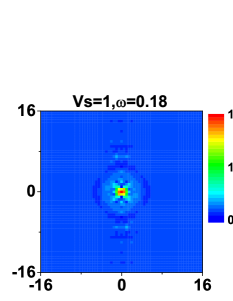
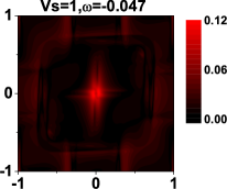
Then we plot the image map of the FC-LDOS in the SDW state at selected energies in Fig. 4. We can see that in q space, there appear high intensity lines, the corresponding wave vectors are responsible for the QPI. The interference is nearly equally strong along x-axis and y-axis. At energy $\omega=-0.047$, for SP $Vs=\pm 1$, the high intensity lines near the center are due to the scattering of pockets($P\nu_{i}$,$P\nu^{\prime}_{i}$) to the corresponding squares($L\nu_{i}$). As seen from Fig. 4, for $Vs=-1,\omega=0.18$, the value of the scattering $q$ along the circle is about $|q|=0.5\pi$, consistent with the wave length $4a$ in real space. It also indicates that when bias energy deviate from zero, the underlying band structure is very important.

Figure 5: (color online)Similar to Fig.3, but for SP $Vs=\pm 3$.

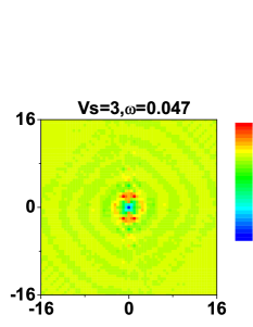
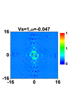
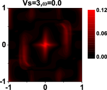
As SP increases to $Vs=\pm 3$, the LDOS at the impurity site decreases rapidly and will vanish for larger SP. Fig. 5 shows that the modulation of the LDOS still exhibits $C_{2}$ symmetry. At $\omega=0.047$, 2D ripple-like pattern appears. From the $q$ space map of $\rho_{q}(\omega)$ in Fig. 6, we note that for strong SP $Vs=\pm 3$, at the Fermi energy, the intra-pocket scattering leads to the two high intensity small arcs near the center. While the scattering between $L\nu_{0}(L\nu_{1})$ and $P\nu_{0},P\nu^{\prime}_{0}(P\nu_{1},P\nu^{\prime}_{1})$ lead to the off-diagonal high intensity spots. For $Vs=-3,\omega=0.0$, away from the center, along the diagonal direction the high intensity arcs arise from inter-pocket scattering(from $P\nu_{i}$ to $P\nu^{\prime}_{i}$) which can be seen clearly from Fig. 6. At $\omega=0.047$, the hight intensity wave vectors along the circle are responsible for the ripple-like modulation in real space. The interplay of FS with the underlying band structure has crucial effect in the scattering process, since the high intensity spots are obviously related to the band structure. For more strong SP, the feature of LDOS and the modulation of LDOS is similar, we also note that for large value of SP, the difference between the repulsive and attractive potentials becomes less obvious.

Figure 6: (color online)Similar to Fig.4, but for SP $Vs=\pm 3$.

IV Quasiparticle interference for larger value of magnetic order

Figure 7: (color online)Panel(a) shows LDOS at the impurity site $(0,0)$ for different scattering potential $Vs=\pm 0.5$ with $m=0.6$. Black dashed line represents LDOS of the bulk, the red solid(blue dot) line corresponds to positive(negative) SP. Panel(b) is similar to (a) with $Vs=\pm 1$.

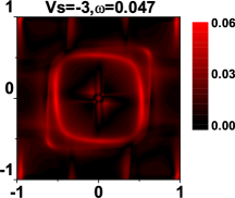
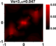
Previous discussions show that the value of magnetic order has high influence on the spectral function, thus we expect it will affect the QPI as well. For larger magnetic order $m=0.6$ and weak SP, at the impurity site, the asymmetry of the LDOS is remarkable. For positive SP $Vs=0.5$, the negative energy peak of the LDOS is much higher than the positive one. While for $Vs=1$ the resonance peak is enhanced and pushed to $\omega=-0.063$, near the Fermi energy. Fig. 7 shows it clearly. On the contrary, for negative SP, the intensity of the overall LDOS is relatively small and the positive energy peak is higher. The most striking feature of the larger-$m$ system is the existence of 1D modulation of the LDOS. Compared to the positive $Vs=1$ case, the 1D structure is more remarkable for $Vs=-1$, as can be seen in Fig. 8. For $Vs=-1$, at selected energies $-0.063$, the 1D stripe pattern is pronounced. The existence of 1D stripe is consistent with the nematic electronic structure observed in the parent compound of the 122 systems chuang which have large magnetic moment.

Figure 8: (color online)Similar to Fig.3, but with $m=0.6$.

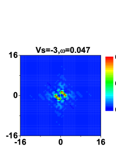
For $m=0.6$, only four pockets are left in the plot of spectral function, which play a important role in the formation of stripe patterns. Responding to the modulation of the LDOS in real space, dispersive excitation in q-space should appear along its perpendicular direction. This is illustrated in Fig. 9, we can see that the dominant high-intensity spots are distributed along a diagonal direction with differently detailed patterns at different energies. For $Vs=-1$, at $\omega=-0.063$, the scattering vector $q\simeq(\pm\pi,\pm\pi)$. They are corresponding to the distance of $\sim 2a$ strip pattern in real space. While the intra-pocket scattering leads to the high intensity spots around the center. Except for the high intensity spots around the center, the high-intensity spots for $Vs=-1$ correspond to the dark ones for $Vs=1$, it means that for repulsive scattering inter-pockets scattering is weak.

Figure 9: (color online)Similar to Fig.4, but with $m=0.6$.

For strong SP $Vs=\pm 3$, the LDOS at some sites in the vicinity of the impurity is strongly affected. Pronounced in-gap resonance peaks appear as shown in Fig. 10. For $Vs=3$, one in-gap peak is located at the negative energy $\omega=-0.031$. While there exist two very close resonance peaks for $Vs=-3$ at the positive energies $\omega=0.047$ and $0.094$, respectively. Those in-gap peaks reflect the formation of bound states induced by QPI. We show the image map of the LDOS in real space at selected energies $\omega=0.047$ and $-0.031$ for $Vs=\pm 3$ in Fig. 11. We can see that, the 1D stripe modulations of the LDOS are remarkable in all cases. The sites with in-gap resonance peaks are located along the lines $y=-x\pm 2$. Fig. 12 shows $\rho_{q}(\omega)$ for $m=0.6,Vs=\pm 3$. As can be seen, at all selected energies the QPI wave vectors are along the diagonal direction, though they form different patterns. For $Vs=3,\omega=-0.031$, the width of the stripe-like pattern is apparently extended since the underlying band structure plays a important role at energies away from zero. For $Vs=-3,\omega=-0.031$, the dominate scattering $q$ is still about $(\pm 0.7\pi,\pm 0.7\pi)$ thus the distance between two stripes in real space is about $2a$.

Figure 10: (color online)Panel(a) shows LDOS at the different sites for $Vs=3$ with $m=0.6$. Black dashed line represents LDOS in bulk, the red solid line represents the site $(2,0)$, and the violet dash dot line represents impurity site. Panel(b) is similar to (a) with $Vs=-3$.

Figure 11: (color online)Similar to Fig.8, but for SP $Vs=\pm 3$.

Figure 12: (color online)Similar to Fig.9, but for SP $Vs=\pm 3$.

For unitary case, LDOS is identity for positive and negative SP. Our calculations show that at low energy $\omega=0.016$, the spatial modulation of the LDOS still has stripe pattern. However, at higher energy $\omega=0.187$, beside the 1D high-intensity stripes there are two circles around the impurity. The dispersion pattern evolves with energy, at high energy $\omega=0.187$ the pattern changes dramatically and has 2D characteristics. Therefore, the dispersion relation is complex in the multi-band system, and can not be fitted by a simple function as in the cuprates disper .

V summary

We have investigated by the T-matrix method the modulation of LDOS and FC-LDOS in the SDW state of the iron-pnictides induced by QPI for different impurity strength and well explained the two experimental works[chuang, ,xiaodong, ]. QPI is sensitive to the value of the magnetic order which may vary from one compound to another.

For small magnetic order, beside the high intensity small pockets aligning along the diagonal direction, the zero-energy spectral function exhibits high-intensity squares around the $\Gamma$ point, therefore it is easy to form 2D QPI patterns. Our calculations show that the 2D patterns of LDOS exist in real- and q-space for various SPs. The exact pattern varies with the energy and in some cases QPI induces ripple-like Friedel oscillations. It is consistent with what have been observed in the $1111$ compound. xiaodong

For larger magnetic order, the main feature of the spatial modulation of the LDOS is the 1D structure at the energies lower than SDW gap. The QPI pattern in momentum space also supports the formation of unidirectional nanostructures chuang . Negative SP favors the inter-pocket scattering more than the repulsive one. The LDOS on some sites in the vicinity of the impurity shows sharp in-gap resonance peaks since the corresponding ungaped Fermi surfaces are enlarged and scattering have more probability to induce excitation at low energies. Our calculations show that remarkable 1D stripe structure aligns along the FM direction in real space. The reason is that for large-m system, zero-energy spectral function has four isolated pockets along the AFM direction. In addition, the topological analysis [yingr, ] of a two-band model and a $5$-band model showed that the stable ungaped Fermi pockets are along the AFM direction thus we expect the QPI obtained in those models should have 1D stripe structure along the FM direction in real space, similar to our results.

Our model has $C_{4}$ symmetry around As iron, both the impurity and SDW could reduce the symmetry to $C_{2}$. The ungaped Fermi pockets as well as the underlying band structure have contribution to the QPI at bias energies away from zero. We obtain the 1D and 2D QPI patterns observed by experiments based on one phenomenological model, the microscopic origin of 1D and 2D QPI patterns is the shape of spectral function at low energies.

VI acknowledgements

The authors would like to thank S. H. Pan, Ang Li and Jian Li for useful discussions. This work was supported by the Texas Center for Superconductivity at the University of Houston and by the Robert A. Welch Foundation under Grant No. E-1146. Huang also acknowledges the support of Shanghai Leading Academic Discipline Project S30105 and Shanghai Education Development Project.

References

- (1) Y. Kamihara, T. Watanabe, M. Hirano and H. Hosono, J. Am. Chem. Soc. 130, 3296 (2008).
- (2) Z.-A Ren, G.-C.Che, X.-L. Dong, J. Yang, W. Lu, W. Yi, X.-L. Shen,Z.-C. Li, L.-L. Sun, F. Zhou, and Z.-X Zhao, Europhys. Lett. 83, 17002 (2008).
- (3) X. H. Chen, T. Wu, G. Wu, R. H. Liu, H. Chen, and D. F. Fang , Nature (London) 453, 761 (2008).
- (4) C. de la Cruz, Q. Huang, J. W. Lynn, Jiying Li, W. Ratcliff II, J. L. Zarestky, H. A. Mook, G. F. Chen, J. L. Luo, N. L. Wang, and Pengcheng Dai , Nature (London) 453, 899 (2008).
- (5) G. F. Chen, Z. Li, D. Wu, G. Li, W. Z. Hu, J. Dong, P. Zheng, J. L. Luo, and N. L. Wang, Phys. Rev. Lett. 100, 247002 (2008).
- (6) M. Rotter, M. Tegel, D. Johrendt, I. Schellenberg, W. Hermes, and R. Pöttgen, Phys. Rev. B. 78, 0020503(R) (2008).
- (7) N. Ni, M. E. Tillman, J.-Q. Yan, A. Kracher, S. T. Hannahs, S. L. Bud’ko, and P. C. Canfield, Phys. Rev. B. 78, 214515 (2008).
- (8) J.-H. Chu, J. G. Analytis, C. Kucharczyk, and I. R. Fisher, Phys. Rev. B 79, 014506 (2009).
- (9) Clarina de la Cruz, Q. Huang, J. W. Lynn, Jiying Li, W. Ratcliff II, J. L. Zarestky, H. A. Mook, G. F. Chen, J. L. Luo, N. L. Wang, and Pengcheng Dai, Nature (London) 453, 899 (2008).
- (10) Jun Zhao, Q. Huang, Clarina de la Curz, J. W. Lynn, M. D. Lumsden, Z. A. Ren, Jie Yang, Xiaolin Shen, Xiaoli Dong, Zhongxian Zhao, and Pengcheng Dai, Phys. Rev. B 78, 132504 (2008).
- (11) Q. Huang, Y. Qiu, Wei Bao, M. A. Green, J. W. Lynn, Y. C. Gasparovic, T. Wu, G. Wu, and X. H. Chen, Phys. Rev. Lett. 101, 257003 (2008).
- (12) Helmut Eschrig, Alexander Lankau, and Klaus Koepernik, Phy, Rev. B 81,155447(2010).
- (13) Chang Liu, Yongbin Lee, A. D. Palczewski, J.-Q. Yan, Takeshi Kondo, B. N. Harmon, R. W. McCallum, T. A. Lograsso, and A. Kaminski, Phy, Rev. B 82,075135(2010).
- (14) L. X. Yang, B. P. Xie, Y. Zhang, C. He, Q. Q. Ge, X. F. Wang, X. H. Chen, M. Arita, J. Jiang, K. Shimada, M. Taniguchi, I. Vobornik, G. Rossi, J. P. Hu, D. H. Lu, Z. X. Shen, Z. Y. Lu, D. L. Feng, Phys. Rev. B 82, 104519 (2010)
- (15) F. Massee, Phy. Rev. B 80,140507(2009),79,220517(2009).
- (16) V. B. Nascimento, Phy, Rev. Lett. 103,076104(2009).
- (17) H. Zhang, Phy. Rev. B 81,104520(2010).
- (18) T.-M. Chuang, M. P. Allan, J. Lee, Y. Xie, N. Ni, S. L. Bud’ko, G. S. Boebinger, P. C. Canfield, J. C. Davis, Science, 327, 181 (2010).
- (19) Xiaodong Zhou, Cun Ye, Peng Cai, Xiangfeng Wang, Xianhui Chen, and Yayu Wang, Phy, Rev. Lett. 106,087001(2011).
- (20) Eduardo Fradkin and Steven A.Kivelson, Science, 327, 155 (2010).
- (21) T. Hanaguri, C. Lupien, Y .Kohsaka, D.-H Lee, M. Azuma, M. Takano, H. Takagi, and J. C. Davis, Nature(London)430, 1001(2004).
- (22) H. Zhai, F. Wang and D. H. Lee, Phy, Rev. B 80,064517 (2009)
- (23) W. C. Lee and C. J. Wu, Phy, Rev. Lett 103,176101 (2009)
- (24) Qiang Han and Z. D. Wang, New. J. Phys 11, 025022 (2009).
- (25) J. Knolle, I. Eremin, A. Akbari ,and R. Moessner, Phys. Rev. Lett 104, 257001 (2010).
- (26) Eugeniu Plamadeala, T. Pereg-Barnea, and Gil Refael, Phys. Rev. B 81, 134513 (2010).
- (27) A. Akbari, J. Knolle,I. Eremin, and R. Moessner, Phys. Rev. B 82, 224506 (2010).
- (28) Tao Zhou, Huaixiang Huang, Yi Gao, Jian-Xin Zhu, and C. S. Ting, Phys. Rev. B 83, 214502 (2011).
- (29) I. I. Mazin, Simon A. J. Kimber, and Dimitri N. Argyriou, Phys. Rev. B 83, 052501 (2011).
- (30) Degang Zhang, Phy. Rev. Lett. 103, 186402 (2009); 104, 089702 (2010).
- (31) A. V. Balatsky, I. Vekhter, Jian-Xin Zhu, Rev. Mod. Phys. 78,373 (2006).
- (32) Degang Zhang and C. S. Ting, Phys. Rev. B 79, 092501 (2009).
- (33) Degang Zhang, C. S. Ting, and C.-R. Hu, Phys. Rev. B 71, 064521 (2005).
- (34) H. Ding, P. Richard, K. Nakayama, T. Sugawara, T. Arakane, Y. Sekiba, A. Takayama, S. Souma, T. Sato, T. Takahashi, Z. Wang, X. Dai, Z. Fang, G. F. Chen, J. L. Luo, and N. L. Wang, Europhys. Lett. 83, 47001 (2008).
- (35) D. H. Lu, M. Yi, S.-K. Mo, A. S. Erickson, J. Analytis, J.-H. Chu, D. J. Singh, Z. Hussain, T. H. Geballe, I. R. Fisher, and Z.-X. Shen, Nature (London) 455, 81 (2008).
- (36) C. Liu, G. D. Samolyuk, Y. Lee, N. Ni, T. Kondo, A. F. Santander-Syro, S. L. Bud’ko, J. L. McChesney, E. Rotenberg, T. Valla, A. V. Fedorov, P. C. Canfield, B. N. Harmon, and A. Kaminski , Phys. Rev. Lett. 101,177005 (2008).
- (37) T. Kondo, A. F. Santander-Syro, O. Copie, Chang Liu, M. E. Tillman, E. D. Mun, J. Schmalian, S. L. Bud’ko, M. A. Tanatar, P. C. Canfield, and A. Kaminski , Phys. Rev. Lett. 101, 147003 (2008).
- (38) K. Terashima, Y. Sekiba, J. H. Bowen, K. Nakayama, T. Kawahara, T. Sato, P. Richard, Y.-M. Xu, L. J. Li, G. H. Cao, Z.-A. Xu, H. Ding, and T. Takahashi, PNAS 106, 7330 (2009).
- (39) Tao Zhou, Degang Zhang, and C. S. Ting, Phys. Rev. B 81, 052506 (2010).
- (40) Yi Gao, Tao Zhou, C. S. Ting, and Wu-Pei Su, Phys. Rev. B 82, 104520 (2010).
- (41) Yi Gao, Huai-Xiang Huang, Chun Chen, C. S. Ting, and Wu-Pei Su, Phys. Rev. Lett. 106, 027004 (2011).
- (42) Huaixiang Huang, Degang Zhang, Tao Zhou, and C. S. Ting, Phys. Rev. B 83, 134517 (2011)
- (43) Y. Sekiba, T. Sato, K. Nakayama, K. Terashima, P. Richard, J. H. Bowen, H. Ding, Y.-M. Xu, L. J. Li, G. H. Cao, Z.-A. Xu, and T. Takahashi, New J. Phys. 11, 025020 (2009).
- (44) K. Matan et al., Phys. Rev. B 82, 054515 (2010).
- (45) S. H. Pan and A. Li, private communication.
- (46) P. Richard, K. Nakayama, T. Sato, M. Neupane, Y.-M. Xu, J. H. Bowen, G. F. Chen, J. L. Luo, N. L. Wang, X. Dai, Z. Fang, H. Ding, and T. Takahashi, Phys. Rev. Lett. 104, 137001 (2010).
- (47) M. F. Crommie, C. P. Lutz, and D. M. Eigler, Nature 363, 524 (1993).
- (48) Ying Ran, Fa Wang, Hui Zhai, Vshvin Vishwanath, and Dung-Hai Lee. 79, 014505 (2009).