Markov properties for mixed graphs

Abstract

In this paper, we unify the Markov theory of a variety of different types of graphs used in graphical Markov models by introducing the class of loopless mixed graphs, and show that all independence models induced by $m$-separation on such graphs are compositional graphoids. We focus in particular on the subclass of ribbonless graphs which as special cases include undirected graphs, bidirected graphs, and directed acyclic graphs, as well as ancestral graphs and summary graphs. We define maximality of such graphs as well as a pairwise and a global Markov property. We prove that the global and pairwise Markov properties of a maximal ribbonless graph are equivalent for any independence model that is a compositional graphoid.

and

1 Introduction

1.1 Introduction and motivation

Graphical Markov models have become widely used in recent years. The models use graphs to represent conditional independence relations for systems of random variables, with nodes of the graph corresponding to random variables and edges representing dependencies. Several classes of graphs with various independence interpretations have been described in the literature. These range from undirected graphs with simple separation for derivation of independencies [19] to various forms of mixed graphs [18, 24, 30], including chain graphs with several different separation criteria [10, 5, 17, 2, 8].

In spite of the differences among these graphs, their structural similarities motivate an attempt to unify them. For this purpose, we introduce the class of loopless mixed graphs and let them entail independence models using the same separation criterion, $m$-separation. This unification covers many graphical independence models in the literature with some independence models for chain graphs forming a notable exception; see Section 4 for further details. We show that any independence model generated by $m$-separation in a loopless mixed graph is a compositional graphoid. This ensures that certain intuitive methods of reasoning are indeed valid for such graphs, as they in some sense behave as ordinary undirected graphs.

A common motivation for defining MC-graphs [18], summary graphs [30], and ancestral graphs [24], is to represent independence relations implied by marginalisation over and conditioning on sets of variables satisfying the Markov property of a directed acyclic graph (DAG). The focus of our study is on a subclass of loopless mixed graphs which we shall term ribbonless. The class of ribbonless graphs is sufficiently rich to serve the same purpose: these graphs are obtained by a simple modification of MC graphs derived from a DAG after marginalisation and conditioning; and it contains summary graphs and ancestral graphs as special cases.

For ribbonless graphs, we define global and pairwise Markov properties, the latter being associated with interpreting missing edges in the graph as representing conditional independencies. We prove as our main result that a compositional graphoid independence model over a maximal ribbonless graph satisfies the global Markov property if and only if it satisfies the pairwise Markov property. This ensures that the independence models represented by such graphs are generated by their missing edges, which again supports the direct visual intuition.

1.2 Some early results on Markov properties

The concepts of pairwise and global Markov properties for undirected graphs were introduced in [13] in the context of random fields and shown to be equivalent for positive densities. Alternative proofs were later given independently by several authors, for example [12, 3]; see also [4]. An abstract variant of this theorem was proven in [21] for independence models satisfying graphoid axioms as these are satisfied by probabilistic distributions with positive densities; see also [29] and [11]. Independence models for undirected graphs were discussed comprehensively in Chapter 3 of [19].

A global Markov property that uses the $m$-separation criterion and a pairwise Markov property were defined in [24] for maximal ancestral graphs without considering conditions under which they are equivalent. We use a generalisation of these Markov properties for maximal ribbonless graphs, which contains maximal ancestral graphs as a subclass, and prove their equivalence for compositional graphoids. This has been mentioned as a conjecture in [14].

1.3 Structure of the paper

In the next section, we introduce the basic concepts of graph theory, general and probabilistic independence models, and compositional graphoids.

In Section 3, we introduce the class of loopless mixed graphs and additional graph theoretical definitions special to mixed graphs. We also associate the $m$-separation criterion to this class, and prove for any loopless mixed graph that the independence model induced by $m$-separation is a compositional graphoid.

In Section 4, we introduce the class of ribbonless graphs and the concept of anterior graphs. We describe the relations between these as well as subclasses of loopless mixed graphs that have been discussed in the literature.

In Section 5, we introduce the concept of maximality by demanding that any additional edge will change the independence model. It is shown that ribbonless graphs are not necessarily maximal, and conditions for maximality are given.

In Section 6, we define a pairwise and a global Markov property for independence models for ribbonless graphs, and prove our main result: that pairwise and global Markov properties are equivalent for compositional graphoid independence models over maximal ribbonless graphs.

2 Basic definitions and concepts

In this section, we introduce basic definitions and notation for independence models, graphs, and compositional graphoids.

2.1 Basic graph theoretical definitions

A graph $G$ is a triple consisting of a node set or vertex set $V$, an edge set $E$, and a relation that with each edge associates two nodes (not necessarily distinct), called its endpoints. When nodes $i$ and $j$ are the endpoints of an edge, they are adjacent and we write $i\sim j$. We say the edge is between its two endpoints. We usually refer to a graph as an ordered pair $G=(V,E)$. Graphs $G_{1}=(V_{1},E_{1})$ and $G_{2}=(V_{2},E_{2})$ are called equal if $(V_{1},E_{1})=(V_{2},E_{2})$. In this case we write $G_{1}=G_{2}$.

Notice that our graphs are labeled, that is, every node is considered as a different object. Hence, for example, graph $i\,\frac{\hskip 4.89998pt\hskip 4.89998pt\;}{\hskip 4.89998pt\hskip 4.89998pt}\,j\,\frac{\hskip 4.89998pt\hskip 4.89998pt\;}{\hskip 4.89998pt\hskip 4.89998pt}\,k$ is not equal to $j\,\frac{\hskip 4.89998pt\hskip 4.89998pt\;}{\hskip 4.89998pt\hskip 4.89998pt}\,i\,\frac{\hskip 4.89998pt\hskip 4.89998pt\;}{\hskip 4.89998pt\hskip 4.89998pt}\,k$.

A loop is an edge with the same endpoints. Multiple edges are edges with the same pair of endpoints. A simple graph has neither loops nor multiple edges.

A subgraph of a graph $G_{1}$ is a graph $G_{2}$ such that $V(G_{2})\subseteq V(G_{1})$ and $E(G_{2})\subseteq E(G_{1})$ and the assignment of endpoints to edges in $G_{2}$ is the same as in $G_{1}$. An induced subgraph by nodes $A\subseteq V$ is a subgraph that contains all and only nodes in $A$ and all edges between two nodes in $A$. A subgraph induced by edges $B\subseteq E$ is a subgraph that contains all and only edges in $B$ and all nodes that are endpoints of edges in $B$.

A walk is a list $\langle v_{0},e_{1},v_{1},\dots,e_{k},v_{k}\rangle$ of nodes and edges such that for $1\leq i\leq k$, the edge $e_{i}$ has endpoints $v_{i-1}$ and $v_{i}$. A path is a walk with no repeated node or edge. If the graph is simple then the path can be uniquely determined by an ordered sequence of node sets. Throughout this paper, we use node sequences to describe paths even in graphs with multiple edges, as it usually is apparent from the context which of multiple edges belong to the path. We say a path is between the first and the last nodes of the list in $G$. We call the first and the last nodes endpoints of the path and all other nodes inner nodes.

If $\pi_{1}=\langle i=i_{0},i_{1},\dots,i_{n},h\rangle$ and $\pi_{2}=\langle h,j_{m},j_{m-1},\dots,j_{0}=j\rangle$ are paths, their combination $\pi_{12}=\pi_{1}\circ\pi_{2}$ is the path $\pi_{12}=\langle i,\ldots,i_{p-1},k,j_{q-1},\dots,j\rangle$, where $k=i_{p}=j_{q}$ is the first node of $\pi_{1}$ which is on both paths. If $k=h$ then $\pi_{12}$ is simply the concatenation of the two paths. In general, the concatenation of two paths will be a walk and not a path as the paths may intersect in more than one point.

A subpath of a path $\pi$ is a path that can be considered a subgraph of $\pi$ with the ordering associated with $\pi$. A cycle in a graph $G$ is a simple subgraph whose nodes can be placed around a circle so that two nodes are adjacent if they appear consecutively along the circle.

2.2 Independence models

An independence model $\mathcal{J}$ over a set $V$ is a set of triples $\langle X,Y\mid Z\rangle$ (called independence statements), where $X$, $Y$, and $Z$ are disjoint subsets of $V$ and $Z$ can be empty, and $\langle\varnothing,Y\mid Z\rangle$ and $\langle X,\varnothing\mid Z\rangle$ always being included in $\mathcal{J}$. The independence statement $\langle X,Y\mid Z\rangle$ is interpreted as “$X$ is independent of $Y$ given $Z$”.

An independence model $\mathcal{J}$ over a set $V$ is a semi-graphoid if for disjoint subsets $A$, $B$, $C$, and $D$ of $V$, it satisfies the four following properties:

1. [3.]

2. $\langle A,B\mid C\rangle\in\mathcal{J}$ if and only if $\langle B,A\mid C\rangle\in\mathcal{J}$ (symmetry);

3. if $\langle A,B\cup D\mid C\rangle\in\mathcal{J}$ then $\langle A,B\mid C\rangle\in\mathcal{J}$ and $\langle A,D\mid C\rangle\in\mathcal{J}$ (decomposition);

4. if $\langle A,B\cup D\mid C\rangle\in\mathcal{J}$ then $\langle A,B\mid C\cup D\rangle\in\mathcal{J}$ and $\langle A,D\mid C\cup B\rangle\in\mathcal{J}$ (weak union);

5. $\langle A,B\mid C\cup D\rangle\in\mathcal{J}$ and $\langle A,D\mid C\rangle\in\mathcal{J}$ if and only if $\langle A,B\cup D\mid C\rangle\in\mathcal{J}$ (contraction).

A semi-graphoid for which the reverse implication of the weak union property holds is said to be a graphoid, that is

1. [5.]

2. if $\langle A,B\mid C\cup D\rangle\in\mathcal{J}$ and $\langle A,D\mid C\cup B\rangle\in\mathcal{J}$ then $\langle A,B\cup D\mid C\rangle\in\mathcal{J}$ (intersection).

Furthermore, a graphoid or semi-graphoid for which the reverse implication of the decomposition property holds is said to be compositional, that is

1. [6.]

2. if $\langle A,B\mid C\rangle\in\mathcal{J}$ and $\langle A,D\mid C\rangle\in\mathcal{J}$ then $\langle A,B\cup D\mid C\rangle\in\mathcal{J}$ (composition).

Notice that simple separation in an undirected graph will trivially satisfy all of these properties, and hence compositional graphoids are direct generalisations of independence models given by separation in undirected graphs.

2.3 Probabilistic conditional independence models

The most common independence models are induced by probability distributions. Consider a set $V$ and a collection of random variables $(X_{\alpha})_{\alpha\in V}$ with state spaces $\mathcal{X}_{\alpha},\alpha\in V$ and joint distribution $P$. We let $X_{A}=(X_{v})_{v\in A}$ etc. for each subset $A$ of $V$. For disjoint subsets $A$, $B$, and $C$ of $V$ we use the short notation $A\perp\!\!\!\perp B\mid C$ to denote that $X_{A}$ is conditionally independent of $X_{B}$ given $X_{C}$ [7, 19], that is, that for any measurable $\Omega\subseteq\mathcal{X}_{A}$ and $P$-almost all $x_{B}$ and $x_{C}$,

$$P(X_{A}\in\Omega\mid X_{B}=x_{B},X_{C}=x_{C})=P(X_{A}\in\Omega\mid X_{C}=x_{C}).$$

We can now induce an independence model $\mathcal{J}(P)$ by letting

$$\langle A,B\mid C\rangle\in\mathcal{J}(P)\quad\mbox{if and only if}\quad A\perp\!\!\!\perp B\mid C\qquad\mbox{w.r.t. }P.$$

We say that an independence model $\mathcal{J}$ is probabilistic if there is a distribution $P$ such that $\mathcal{J}=\mathcal{J}(P)$. We then also say that $P$ is faithful to $\mathcal{J}$.

Probabilistic independence models are always semi-graphoids [21], whereas the converse is not necessarily true; see [29]. If $P$ has strictly positive density, the induced independence model is also a graphoid; see, for example, Proposition 3.1 in [19]. If the distribution $P$ is a regular multivariate Gaussian distribution, $\mathcal{J}(P)$ is a compositional graphoid. This follows from the fact that for such a distribution

$$A\perp\!\!\!\perp B\mid C\quad\iff\quad k^{\alpha\beta}_{A\cup B\cup C}=0\qquad\mbox{for all }\alpha\in A,\beta\in B,$$

where $k^{\alpha\beta}_{A\cup B\cup C}$ is the $\alpha\beta$ entry in the concentration matrix of the distribution of $X_{A\cup B\cup C}$ and hence setwise conditional independence is directly determined by nodewise conditional independence.

Probabilistic independence models with positive densities are not in general compositional graphoids; this only holds for special types of multivariate distributions such as the Gaussian mentioned above and, say, the symmetric binary distributions used in [32].

3 Independence models for mixed graphs

3.1 Mixed graphs

A mixed graph is a graph containing three types of edges denoted by arrows, arcs (bi-directed edges), and lines (full lines). Notice that we allow multiple edges of the same type. A loopless mixed graph (LMG) is a mixed graph that does not contain any loops (a loop may be line, arrow, or arc). For an arrow $j\hskip 1.49994pt\frac{\hskip 4.89998pt\hskip 4.89998pt}{\hskip 4.89998pt}\!\!\!\!\!\succ\!\hskip 1.50696pti$, we say that the arrow is from $j$ to $i$. We also call $j$ a parent of $i$, $i$ a child of $j$ and we use the notation $\mathrm{pa}(i)$ for the set of all parents of $i$ in the graph. In the cases of $i\hskip 1.49994pt\frac{\hskip 4.89998pt\hskip 4.89998pt}{\hskip 4.89998pt}\!\!\!\!\!\succ\!\hskip 1.50696ptj$ or $i\hskip 0.59998pt\prec\!\!\!\!\!\frac{\hskip 4.89998pt\hskip 4.89998pt}{\hskip 4.89998pt}\!\!\!\!\!\succ\!\hskip 1.50696ptj$, we say that there is an arrowhead at $j$ or pointing to $j$.

A path $\langle i=i_{0},i_{1},\dots,i_{n}=j\rangle$ is direction-preserving from $i$ to $j$ if all $i_{k}i_{k+1}$ edges are arrows pointing from $i_{k}$ to $i_{k+1}$. If there is a direction-preserving path from $j$ to $i$ then $j$ is an ancestor of $i$ and $i$ is a descendant of $j$. We denote the set of ancestors of $i$ by $\operatorname{an}(i)$. Notice that we do not include $i$ in its set of anteriors or descendants.

A tripath is a path with three nodes. Note that [26] used the term V-configuration for such a path. However, here we follow [16] and most texts by letting a V-configuration be a tripath with non-adjacent endpoints.

In a mixed graph the inner node of three tripaths $i\hskip 1.49994pt\frac{\hskip 4.89998pt\hskip 4.89998pt}{\hskip 4.89998pt}\!\!\!\!\!\succ\!\hskip 1.50696ptt\hskip 0.50003pt\prec\!\!\!\!\!\frac{\hskip 4.89998pt\hskip 4.89998pt}{\hskip 4.89998pt}\hskip 1.99997ptj$, $i\hskip 0.59998pt\prec\!\!\!\!\!\frac{\hskip 4.89998pt\hskip 4.89998pt}{\hskip 4.89998pt}\!\!\!\!\!\succ\!\hskip 1.50696ptt\hskip 0.50003pt\prec\!\!\!\!\!\frac{\hskip 4.89998pt\hskip 4.89998pt}{\hskip 4.89998pt}\hskip 1.99997ptj$, and $i\hskip 0.59998pt\prec\!\!\!\!\!\frac{\hskip 4.89998pt\hskip 4.89998pt}{\hskip 4.89998pt}\!\!\!\!\!\succ\!\hskip 1.50696ptt\hskip 0.59998pt\prec\!\!\!\!\!\frac{\hskip 4.89998pt\hskip 4.89998pt}{\hskip 4.89998pt}\!\!\!\!\!\succ\!\hskip 1.50696ptj$ is a collider (or a collider node) and the inner node of any other tripath is a non-collider (or a non-collider node) on the tripath or more generally on any path of which the tripath is a subpath. We shall also say that the tripath itself with inner collider or non-collider node is a collider or non-collider. We may speak of a collider or non-collider without mentioning the relevant tripath or path when this is apparent from the context. Notice that a node may be a collider on one tripath and a non-collider on another.

Two paths $\pi_{1}$ and $\pi_{2}$ (including tripaths or edges) between $i$ and $j$ are called endpoint-identical if there is an arrowhead pointing to $i$ in $\pi_{1}$ if and only if there is an arrowhead pointing to $i$ in $\pi_{2}$ and similarly for $j$. For example, the paths $i\hskip 1.49994pt\frac{\hskip 4.89998pt\hskip 4.89998pt}{\hskip 4.89998pt}\!\!\!\!\!\succ\!\hskip 1.50696ptj$, $i\,\frac{\hskip 4.89998pt\hskip 4.89998pt\;}{\hskip 4.89998pt\hskip 4.89998pt}\,k\hskip 0.59998pt\prec\!\!\!\!\!\frac{\hskip 4.89998pt\hskip 4.89998pt}{\hskip 4.89998pt}\!\!\!\!\!\succ\!\hskip 1.50696ptj$, and $i\hskip 1.49994pt\frac{\hskip 4.89998pt\hskip 4.89998pt}{\hskip 4.89998pt}\!\!\!\!\!\succ\!\hskip 1.50696ptk\hskip 0.50003pt\prec\!\!\!\!\!\frac{\hskip 4.89998pt\hskip 4.89998pt}{\hskip 4.89998pt}\hskip 1.99997ptl\hskip 0.59998pt\prec\!\!\!\!\!\frac{\hskip 4.89998pt\hskip 4.89998pt}{\hskip 4.89998pt}\!\!\!\!\!\succ\!\hskip 1.50696ptj$ are all endpoint-identical as they have an arrowhead pointing to $j$ but no arrowhead pointing to $i$ on the paths.

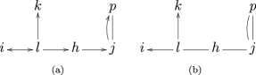
Figure 1: (a) A mixed graph $G$. (b) The anterior graph $G^{*}$ of $G$.

3.2 Anterior graphs and sets

The anterior graph of a loopless mixed graph $G$, denoted by $G^{*}$, is the graph obtained from $G$ by recursively removing arrowheads pointing to nodes that are the endpoints of a line, that is, by obtaining $\,\frac{\hskip 4.89998pt\hskip 4.89998pt\;}{\hskip 4.89998pt\hskip 4.89998pt}\,\circ\,\frac{\hskip 4.89998pt\hskip 4.89998pt\;}{\hskip 4.89998pt\hskip 4.89998pt}\,$ and $\hskip 0.50003pt\prec\!\!\!\!\!\frac{\hskip 4.89998pt\hskip 4.89998pt}{\hskip 4.89998pt}\hskip 1.99997pt\circ\,\frac{\hskip 4.89998pt\hskip 4.89998pt\;}{\hskip 4.89998pt\hskip 4.89998pt}\,$ from $\hskip 1.49994pt\frac{\hskip 4.89998pt\hskip 4.89998pt}{\hskip 4.89998pt}\!\!\!\!\!\succ\!\hskip 1.50696pt\circ\,\frac{\hskip 4.89998pt\hskip 4.89998pt\;}{\hskip 4.89998pt\hskip 4.89998pt}\,$ and $\hskip 0.59998pt\prec\!\!\!\!\!\frac{\hskip 4.89998pt\hskip 4.89998pt}{\hskip 4.89998pt}\!\!\!\!\!\succ\!\hskip 1.50696pt\circ\,\frac{\hskip 4.89998pt\hskip 4.89998pt\;}{\hskip 4.89998pt\hskip 4.89998pt}\,$ respectively. Hence, it holds that $G=G^{*}$ if and only if there are no arrowheads pointing to lines in $G$. Notice also that since removing an arrowhead pointing to a line does not affect other arrowheads pointing to lines, it does not matter which arrowhead is removed first; therefore, the order of removing arrowheads pointing to lines does not affect the final graph obtained.

A path $\langle i=i_{0},i_{1},\dots,i_{n}=j\rangle$ from $i$ to $j$ ($i\neq j$) in $G^{*}$ is an anterior path if it has the form $i\,\frac{\hskip 4.89998pt\hskip 4.89998pt\;}{\hskip 4.89998pt\hskip 4.89998pt}\,i_{1}\,\frac{\hskip 4.89998pt\hskip 4.89998pt\;}{\hskip 4.89998pt\hskip 4.89998pt}\,\cdots\,\frac{\hskip 4.89998pt\hskip 4.89998pt\;}{\hskip 4.89998pt\hskip 4.89998pt}\,i_{m}\hskip 1.49994pt\frac{\hskip 4.89998pt\hskip 4.89998pt}{\hskip 4.89998pt}\!\!\!\!\!\succ\!\hskip 1.50696pti_{m+1}\hskip 1.49994pt\frac{\hskip 4.89998pt\hskip 4.89998pt}{\hskip 4.89998pt}\!\!\!\!\!\succ\!\hskip 1.50696pt\cdots\hskip 1.49994pt\frac{\hskip 4.89998pt\hskip 4.89998pt}{\hskip 4.89998pt}\!\!\!\!\!\succ\!\hskip 1.50696ptj$. Notice that this path may only contain lines or arrows. We shall say that $i$ is anterior of $j$ in $G$ if there is an anterior path from $i$ to $j$ in $G^{*}$. Notice that although the anterior path is defined in $G^{*}$ we may from time to time refer to an anterior path in $G$ as the path corresponding to the anterior path in $G^{*}$.

We use the notation $\operatorname{ant}(i)$ for the set of all anteriors of $i$. Notice that, since ancestral graphs have no arrowheads pointing to lines, we have $G=G^{*}$ for an ancestral graph. Thus, our definition of anterior extends the notion of anterior used in [24] for ancestral graphs with the minor difference that we do not include a node in its anterior set. However, it is different from and inconsistent with the definition of anteriors in [10] and [1].

For example, in the graph $G$ in Figure 1(a), $\operatorname{ant}(i)=\{l,h,j,p\}$ and $\operatorname{ant}(p)=\{l,h,j\}$. This can be seen by looking at the anterior paths $\langle p,j,h,l,i\rangle$ from $p$ to $i$ and $\langle l,h,j,p\rangle$ from $l$ to $p$ (as well as from $p$ to $l$) in Figure 1(b).

We first show that transitivity holds for anteriors.

Lemma 1

For any loopless mixed graph it holds that if $i\in\operatorname{ant}(j)$ and $j\in\operatorname{ant}(k)$ then $i\in\operatorname{ant}(k)$.

[Proof.] If $i\in\operatorname{ant}(j)$ and $j\in\operatorname{ant}(k)$, $G^{*}$ has anterior paths $\pi_{1}$ from $i$ to $j$ and $\pi_{2}$ from $j$ to $k$. As no arrowhead meets a line in $G^{*}$ their combination $\pi_{1}\circ\pi_{2}$ is an anterior path from $i$ to $j$ in $G^{*}$.

Here we also introduce a lemma that is used in several proofs of this paper.

Lemma 2

Let $G$ be a loopless mixed graph. If $i\in\operatorname{ant}(j)\setminus\operatorname{an}(j)$, then either $i$ or a descendant of $i$ is the endpoint of a line in $G$.

[Proof.] The proof uses induction on the number of arrowheads removed from $G$ to obtain $G^{*}$. For the base, if $G=G^{*}$ it follows immediately from the definition of an anterior path that $i$ must be the endpoint of a line or we would have $i\in\operatorname{an}(j)$.

Next, suppose that $G^{*}$ is obtained from $G$ by removing $n+1$ arrowheads and let $\tilde{G}$ be obtained from $G$ by removing a single arrowhead pointing to a line from $G$. Then $G^{*}$ is also the anterior graph of $\tilde{G}$, but with only $n$ arrowheads needing removal. Thus, if $i\in\operatorname{ant}(j)$ in $G$, it is also anterior to $j$ in $\tilde{G}$. Consider now two cases:

Case I. Assume $i$ is an ancestor of $j$ in $\tilde{G}$. Since $i$ is not an ancestor of $j$ in $G$, $\tilde{G}$ must have been obtained by turning an arc into an arrow. Say this arrowhead points to $h$. Then $h$ is an endpoint of a line and it is a descendant of $i$ in $G$.

Case II. If $i$ is not an ancestor of $j$ in $\tilde{G}$, the inductive hypothesis yields that $i$ is either adjacent to a line $ih$ in $\tilde{G}$ or has a descendant $h$ in $\tilde{G}$ which is the endpoint of a line in $\tilde{G}$. Let $h$ be the node adjacent to a line in $\tilde{G}$. If the arrowhead removed is not on the direction-preserving path $\pi$ from $i$ to $h$ the conclusion obviously follows. Else, there must be node $k$ on $\pi$ which is adjacent to a line in $G$ and can be used instead of $h$.

3.3 The $m$-separation criterion

Here we define a separation criterion for LMGs. We use this criterion to induce independencies on LMGs and its subclasses defined in Section 3.

We first define an $m$-connecting path: Let $C$ be a subset of the node set of an LMG. A path is $m$-connecting given $C$ if all its collider nodes are in $C\cup\operatorname{an}(C)$ and all its non-collider nodes are outside $C$. For two disjoint subsets of the node set $A$ and $B$, we say that $C$ $m$-separates $A$ and $B$ if there is no $m$-connecting path between $A$ and $B$ given $C$. In this case, we use the notation $A\perp_{m}B\mid C$. Notice that the $m$-separation criterion induces an independence model $\mathcal{J}_{m}(G)$ on $G$ by $A\perp_{m}B\mid C\iff\langle A,B\mid C\rangle\in\mathcal{J}_{m}(G)$.

We note that $m$-separation is unaffected if we replace multiple edges of the same type with a single edge of that type. The $m$-separation criterion for LMGs is the same as the separation criterion defined in [24]. It is an extension of the $d$-separation criterion introduced in [21]. Clearly, $m$-separation is also an extension of simple separation in an undirected graph, as then all edges are lines.

For example, in graph $G$ in Figure 2 it holds that $h\in\operatorname{an}(l)$ and, thus, $\langle i,h,j\rangle$ is an $m$-connecting path given $l$. Therefore, $\langle i,j\mid l\rangle\notin\mathcal{J}_{m}(G)$.

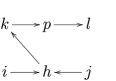
Figure 2: A loopless mixed graph $G$ for which $\langle i,j\mid l\rangle\notin\mathcal{J}_{m}(G)$.

We now have the following theorem. A similar result for the induced independence model for MC graphs was given in Proposition 2.10 of [18].

Theorem 1

For any loopless mixed graph $G$, the independence model $\mathcal{J}_{m}(G)$ is a compositional graphoid.

[Proof.] For $G=(N,F)$ and disjoint subsets $A$, $B$, $C$, and $D$ of $N$, we prove that $\perp_{m}$ satisfies the six compositional graphoid axioms: (

• 6)]

• Symmetry: If $A\perp_{m}B\mid C$, then $B\perp_{m}A\mid C$: If there is no $m$-connecting path between $A$ and $B$ given $C$, then there is no $m$-connecting path between $B$ and $A$ given $C$.

• Decomposition: If $A\perp_{m}(B\cup D)\mid C$, then $A\perp_{m}D\mid C$: If there is no $m$-connecting path between $A$ and $B\cup D$ given $C$, then there is no $m$-connecting path between $A$ and $D\subseteq(B\cup D)$ given $C$.

• Weak union: If $A\perp_{m}(B\cup D)\mid C$ then $A\perp_{m}B\mid(C\cup D)$: From (2) we know that $A\perp_{m}D\mid C$ and $A\perp_{m}B\mid C$. Suppose, for contradiction, that there exist $m$-connecting paths between $A$ and $B$ given $C\cup D$. Consider a shortest path of this type and call it $\pi$. If there is no inner collider node on $\pi$, then there is an $m$-connecting path between $A$ and $B$ given $C$, a contradiction. On $\pi$ all collider nodes are in $(C\cup D)\cup\operatorname{an}(C\cup D)$. If all collider nodes are in $C\cup\operatorname{an}(C)$, then there is an $m$-connecting path between $A$ and $B$ given $C$, again a contradiction. Hence, consider the closest collider node $i\in(D\cup\operatorname{an}(D))\setminus(C\cup\operatorname{an}(C))$ to $A$ on $\pi$. Now since the nodes between $A$ and $i$ are not in $B\cup D$, there is an $m$-connecting path between $A$ and $i$ given $C$. If $i\in D$, then this is obviously a contradiction. Otherwise there is a node $k\in D$, for which $i\in\operatorname{an}(k)$ and thus an $m$-connecting path between $A$ and $k$ given $C$, a contradiction again. Therefore, there is no $m$-connecting path between $A$ and $B$ given $C\cup D$.

• Contraction: If $A\perp_{m}B\mid C$ and $A\perp_{m}D\mid(B\cup C)$, then $A\perp_{m}(B\cup D)\mid C$: Suppose, for contradiction, that there exists an $m$-connecting path between $A$ and $B\cup D$ given $C$. Consider a shortest path of this type and call it $\pi$. The path $\pi$ is either between $A$ and $B$ or between $A$ and $D$. The path $\pi$ being between $A$ and $B$ contradicts $A\perp_{m}B\mid C$. Therefore, $\pi$ is between $A$ and $D$. In addition, since all inner collider nodes on $\pi$ are in $C\cup\operatorname{an}(C)$ and because $A\perp_{m}D\mid(B\cup C)$, an inner non-collider node should be in $B$. This contradicts the fact that $\pi$ is a shortest $m$-connecting path between $A$ and $B\cup D$ given $C$.

• Intersection: If $A\perp_{m}B\mid(C\cup D)$ and $A\perp_{m}D\mid(C\cup B)$, then $A\perp_{m}(B\cup D)\mid C$: Suppose, for contradiction, that there exists an $m$-connecting path between $A$ and $B\cup D$ given $C$. Consider a shortest path of this type and call it $\pi$. The path $\pi$ is either between $A$ and $B$ or between $A$ and $D$. Because of symmetry between $B$ and $D$ in the formulation it is enough to suppose that $\pi$ is between $A$ and $B$. Since all inner collider nodes on $\pi$ are in $C\cup\operatorname{an}(C)$ and because $A\perp_{m}B\mid(C\cup D)$, an inner non-collider node should be in $D$. This contradicts the fact that $\pi$ is a shortest $m$-connecting path between $A$ and $B\cup D$ given $C$.

• Composition: If $A\perp_{m}B\mid C$ and $A\perp_{m}D\mid C$, then $A\perp_{m}(B\cup D)\mid C$: Suppose, for contradiction, that there exist $m$-connecting paths between $A$ and $B\cup D$ given $C$. Consider a path of this type and call it $\pi$. Path $\pi$ is either between $A$ and $B$ or between $A$ and $D$. Because of symmetry between $B$ and $D$ in the formula it is enough to suppose that $\pi$ is between $A$ and $B$. But this contradicts $A\perp_{m}B\mid C$.∎

Theorem 1 implies that we can focus on establishing conditional independence for pairs of nodes, formulated in the corollary below.

Corollary 1

For a loopless mixed graph $G$ and disjoint subsets of its node set $A$, $B$, and $C$, it holds that $A\perp_{m}B\mid C$ if and only if $i\perp_{m}j\mid C$ for every nodes $i\in A$ and $j\in B$.

[Proof.] The result follows from the fact that $\perp_{m}$ satisfies the decomposition and the composition properties.

4 Subclasses of loopless mixed graphs

LMGs and their associated independence models induced by $m$-separation unify a variety of previously discussed graphical independence models.

4.1 Chain graphs

Important exceptions include certain independence models for chain graphs. Chain graphs themselves are LMGs, but at least four different Markov properties for chain graphs have been discussed in the literature. Drton [8] has classified them into (i) the LWF or block concentration Markov property, (ii) the AMP or concentration regression Markov property, (iii) a Markov property that is dual to the AMP Markov property, and (iv) and the multivariate regression Markov property. When the chain components consist entirely of arcs, the multivariate regression property is identical to the one induced by $m$-separation. However, the independence model induced by $m$-separation in a chain graph is typically different from any of the other chain graph interpretations; see also [25, 22] and [20].

4.2 Ribbonless graphs

The class of MC graphs, defined in [18], contains line loops and uses a different separation criterion for inducing an independence model. However, a small modification of any MC graph that is derived from a DAG after marginalisation and conditioning yields a so-called ribbonless graph, which is loopless and induces the same independence model as the MC graph, but by $m$-separation [27]. Any ribbonless graph can be generated from a DAG by marginalisation and conditioning and ribbonless graphs are stable under these operations [26]. The remaining part of this paper deals with such graphs. We first give a formal definition of a ribbon.

A ribbon is a collider tripath $\langle h,i,j\rangle$ such that both of the following two conditions hold:

1. [(2)]

2. there is no endpoint-identical edge between $h$ and $j$, that is, there is no $hj$-arc in the case of $h\hskip 0.59998pt\prec\!\!\!\!\!\frac{\hskip 4.89998pt\hskip 4.89998pt}{\hskip 4.89998pt}\!\!\!\!\!\succ\!\hskip 1.50696pti\hskip 0.59998pt\prec\!\!\!\!\!\frac{\hskip 4.89998pt\hskip 4.89998pt}{\hskip 4.89998pt}\!\!\!\!\!\succ\!\hskip 1.50696ptj$; there is no $hj$-line in the case of $h\hskip 1.49994pt\frac{\hskip 4.89998pt\hskip 4.89998pt}{\hskip 4.89998pt}\!\!\!\!\!\succ\!\hskip 1.50696pti\hskip 0.50003pt\prec\!\!\!\!\!\frac{\hskip 4.89998pt\hskip 4.89998pt}{\hskip 4.89998pt}\hskip 1.99997ptj$; and there is no arrow from $h$ to $j$ in the case of $h\hskip 1.49994pt\frac{\hskip 4.89998pt\hskip 4.89998pt}{\hskip 4.89998pt}\!\!\!\!\!\succ\!\hskip 1.50696pti\hskip 0.59998pt\prec\!\!\!\!\!\frac{\hskip 4.89998pt\hskip 4.89998pt}{\hskip 4.89998pt}\!\!\!\!\!\succ\!\hskip 1.50696ptj$;

3. $i$ or a descendant of $i$ is the endpoint of a line or is on a direction-preserving cycle.

If $i$ or a descendant of $i$ is the endpoint of a line, then we say the ribbon is straight and if they are on a direction-preserving cycle we say the ribbon is cyclic. A ribbonless graph (RG) is an LMG that has no ribbons as induced subgraphs. Figure 3 illustrates a straight ribbon $\langle h,i,j\rangle$ and the simplest cyclic ribbon.

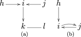
Figure 3: (a) A straight ribbon $\langle h,i,j\rangle$ with $\operatorname{ne}(i)=\varnothing$. (b) The simplest cyclic ribbon $\langle h,i,j\rangle$.

Figure 4(a) illustrates a graph containing a straight ribbon $\langle h,i,j\rangle$ and Figure 4(b) illustrates a ribbonless graph. Notice that $\langle h,i,j\rangle$ is not a ribbon here since there is a line between $h$ and $j$ and this is an endpoint-identical edge.

Figure 4: (a) A graph that is not ribbonless. (b) A ribbonless graph.

We proceed to establish that ribbonless graphs yield identical independence models to their anterior graphs and need the following lemma.

Lemma 3

Let $G$ be a ribbonless graph. If there is a collider tripath $\langle i,j,k\rangle$ in $G$ that is non-collider in $G^{*}$, then $G$ has an $ik$-edge that is endpoint-identical to $\langle i,j,k\rangle$.

[Proof.] Suppose that $\langle G=G_{0},G_{1},\dots,G_{n}=G^{*}\rangle$ is a sequence of graphs, where each graph has been generated by removing one arrowhead pointing to a full line from the previous graph starting from $G$.

Consider the first intermediate graph $G_{p+1}$ where $\langle i,j,k\rangle$ turns into a non-collider tripath. We prove by reverse induction that, for each $0\leq q\leq p$, $\langle i,j,k\rangle$ is a straight ribbon unless there is an endpoint-identical $ik$-edge to $\langle i,j,k\rangle$.

In $G_{p}$, the node $j$ is obviously the endpoint of a line and the result holds. Thus, we assume that the result holds for $G_{q}$. In $G_{q-1}$, it is easy to observe that if the line that makes the ribbon is an arrow pointing to another line or if an arrow on the direction-preserving cycle pointing to a line is an arc then $j$ or a descendant of $j$ is still the endpoint of a line. Therefore, the result holds in $G_{q-1}$. Therefore, by reverse induction, this result holds in $G$, and since $G$ is ribbonless, in $G$ there is an endpoint-identical $ik$-edge to $\langle i,j,k\rangle$. For the graph $G$ in Figure 3(a), the anterior graph $G^{*}$ is the graph where all edges become undirected. Clearly there is no endpoint-identical edge $hj$ and the conclusion of Lemma 3 does not hold. This illustrates the role of a graph being ribbonless.

Proposition 0

For a ribbonless graph $G$, it holds that $\mathcal{J}_{m}(G)=\mathcal{J}_{m}(G^{*})$, that is, $G$ and $G^{*}$ are Markov equivalent.

[Proof.] It is enough to prove that there is an $m$-connecting path between $i$ and $j$ given $C$ in $G$ if and only if there is an $m$-connecting path between $i$ and $j$ given $C$ in $G^{*}$.

Suppose that there is an $m$-connecting path between $i$ and $j$ given $C$ in $G$. All non-colliders on the path in $G$ are preserved in $G^{*}$. In addition, by Lemma 3, a collider tripath $\langle i,j,k\rangle$ becomes non-collider if there is an endpoint-identical $ik$-edge to $\langle i,j,k\rangle$. In this case, the $ik$-edge can be used instead of $\langle i,j,k\rangle$ to establish an $m$-connecting path in $G^{*}$.

Conversely, suppose that there is an $m$-connecting path between $i$ and $j$ given $C$ in $G^{*}$. Collider tripaths are collider tripaths in $G$, and if a non-collider tripath $\langle i,j,k\rangle$ has been collider in $G$ then, by Lemma 3, one can again use the $ik$-edge instead of $\langle i,j,k\rangle$. Thus the only thing that remains to be proven is that a direction-preserving path pointing to a member of $C$ in $G$ remains direction-preserving in $G^{*}$.

In this case, by the same argument as in Lemma 3, if for the collider tripath $\langle i,j,k\rangle$, where $j\in\operatorname{an}(C)$, the arrowhead of an arrow on the direction-preserving path in $G$ is taken away then $\langle i,j,k\rangle$ is a ribbon unless there is an endpoint-identical $ik$-edge to $\langle i,j,k\rangle$. Hence, we can use the $ik$-edge instead of $\langle i,j,k\rangle$ to establish an $m$-connecting path.

Thus, the absence of ribbons ensures that the Markov property is unchanged by forming the anterior graph $G^{*}$. Again, as the anterior graph $G^{*}$ of the graph $G$ in Figure 3(a) is the graph with all edges becoming undirected, we have $h\perp_{m}j$ in $G$ but not $h\perp_{m}j$ in $G^{*}$, illustrating that absence of ribbons is essential for the Markov equivalence of $G$ and $G^{*}$.

Independence models induced by $m$-separation in a ribbonless graph can be induced by marginalisation over and conditioning on a DAG-independence model [26]. This implies that independence models corresponding to RGs are probabilistic, that is, any RG has a faithful probability distribution.

4.3 Other subclasses of loopless mixed graphs

Other subclasses of LMGs that use $m$-separation and have been discussed in the literature are summary graphs [30], ancestral graphs [24], acyclic directed mixed graphs [28, 23], undirected or concentration graphs [6, 19], bidirected or covariance graphs [5, 15, 31, 9], and the class of directed acyclic graphs [16, 21, 11]. In papers on summary graphs and regression chain graphs, dashed undirected edges (without arrowheads) have often been used in place of bi-directed edges. Using the latter as we have done here makes the idea of a collider more immediate so $m$-separation can be used directly and the relation between the various types of graphs becomes transparent.

The use of some of the above graphs are motivated by representing independence models obtained by marginalisation over and conditioning on subsets of the node set of a DAG. For those graphs, arcs indicate marginalisation and lines indicate conditioning.

The diagram in Figure 5 illustrates the hierarchy of subclasses of LMGs and their associated independence models generated by $m$-separation. For example, it can be seen from the diagram that bidirected graphs are also ancestral graphs, since they form a subclass of multivariate regression chain graphs, which again form a subclass of ancestral graphs. Notice that the associated classes of independence models are all distinct except for ancestral, summary, and ribbonless graphs, which are alternative representations of the same class of independence models.

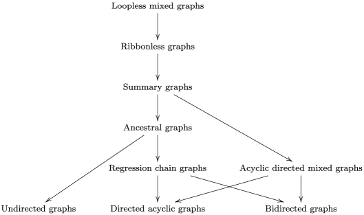
Figure 5: The hierarchy of subclasses of LMGs.

5 Maximal ribbonless graphs

Among the independence models over the node set $V$ of a graph $G$, those that are of interest to us conform with $G$, meaning that $i\sim j$ in $G$ implies $\langle i,j\mid C\rangle\notin\mathcal{J}$ for any $C\subseteq V\setminus\{i,j\}$. Henceforth, we assume that independence models $\mathcal{J}$ conform with $G$, unless otherwise stated.

For example, the independence model $\mathcal{J}=\{\langle i,l\mid j\rangle,\langle i,k\mid\varnothing\rangle\}$ conforms with the graph $G$ in Figure 6, whereas $\mathcal{J}=\{\langle i,l\mid j\rangle,\langle i,j\mid\varnothing\rangle\}$ does not conform with $G$ because of the independence statement $\langle i,j\mid\varnothing\rangle$.

Figure 6: The independence model $\mathcal{J}=\{\langle i,l\mid j\rangle,\langle i,k\mid\varnothing\rangle\}$ conforms with $G$ whereas $\mathcal{J}=\{\langle i,l\mid j\rangle,\langle i,j\mid\varnothing\rangle\}$ does not.

A ribbonless graph $G$ is called maximal if by adding any edge to $G$, the independence model induced by $m$-separation changes. Note that in [30] a graph that is maximal is called an independence graph.

The independence models on RGs induced by $m$-separation conform with the graphs; hence for maximal graphs, adding an edge to the graph makes the independence model smaller. Therefore, we have the lemma below.

Lemma 4

A graph $G=(V,E)$ is maximal if and only if for every pair of non-adjacent nodes $i$ and $j$ of $V$, there exists a subset $C$ of $V\setminus\{i,j\}$ such that $i\perp_{m}j\mid C$.

[Proof.] The result follows directly from the definition of maximality.

RGs are not maximal in general. To see this consider the RG in Figure 7. There is no $C$ such that $i\perp_{m}j\mid C$. This is because if $k\in C$, the path $i\hskip 1.49994pt\frac{\hskip 4.89998pt\hskip 4.89998pt}{\hskip 4.89998pt}\!\!\!\!\!\succ\!\hskip 1.50696ptk\hskip 0.59998pt\prec\!\!\!\!\!\frac{\hskip 4.89998pt\hskip 4.89998pt}{\hskip 4.89998pt}\!\!\!\!\!\succ\!\hskip 1.50696ptj$ is $m$-connecting given $C$, and if $k\notin C$, $i\hskip 1.49994pt\frac{\hskip 4.89998pt\hskip 4.89998pt}{\hskip 4.89998pt}\!\!\!\!\!\succ\!\hskip 1.50696ptk\hskip 1.49994pt\frac{\hskip 4.89998pt\hskip 4.89998pt}{\hskip 4.89998pt}\!\!\!\!\!\succ\!\hskip 1.50696ptj$ is $m$-connecting given $C$.

Figure 7: A non-maximal RG.

To characterise maximal RGs, we need the following notion: A path $\langle j,q_{1},q_{2},\dots,q_{p},i\rangle$ is a primitive inducing path between $i$ and $j$ if and only if for every $n$, $1\leq n\leq p$,

1. [(ii)]

2. $q_{n}$ is a collider on the path; and

3. $q_{n}\in\operatorname{an}(\{i\}\cup\{j\})$.

This definition is a trivial extension of a primitive inducing path as defined for ancestral graphs in [24]. Note in particular that we consider any edge between $i$ and $j$ to be a primitive inducing path. In Figure 7, $\langle i,k,j\rangle$ is a primitive inducing path.

Next, we need the following lemmas. These also establish a pairwise Markov property for maximal RGs.

Lemma 5

A non-collider node $k$ on a path $\pi$ between $i$ and $j$ in a ribbonless graph $G$ is either in $\operatorname{ant}(i)\cup\operatorname{ant}(j)$ or an anterior of a collider node $h$ on $\pi$. Moreover, the relevant subpath of $\pi$ between $k$ and $i$, $j$ or $h$ is an anterior path in $G^{*}$.

[Proof.] Let $k=i_{m}$ be a non-collider node on a path $\pi=\langle i=i_{0},i_{1},\dots,i_{n}=j\rangle$ in $G$. Then from at least one side (say from $i_{m-1}$) there is no arrowhead on $\pi$ pointing to $k$. By moving towards $i$ on the path as long as $i_{p}$, $1\leq p\leq m-1$, is non-collider on the path, we obtain that $k\in\operatorname{ant}(i_{p-1})$. This implies that if no $i_{p}$ is a collider then $k\in\operatorname{ant}(i)$ and hence the lemma follows.

Lemma 6

For nodes $i$ and $j$ in an RG that are not connected by any primitive inducing paths (and hence $i\not\sim j$), it holds that $i\perp_{m}j\mid(\operatorname{ant}(i)\cup\operatorname{ant}(j))\setminus\{i,j\}$.

[Proof.] Suppose, for contradiction, there is an $m$-connecting path between $i$ and $j$ given $(\operatorname{ant}(i)\cup\operatorname{ant}(j))\setminus\{i,j\}$ and denote a shortest such path by $\pi$. If there is a non-collider node $k$ on $\pi$ then, by Lemma 5, $k$ is either in $\operatorname{ant}(i)\cup\operatorname{ant}(j)$ or it is an anterior of a collider node on $\pi$. But since $\pi$ is $m$-connecting given $(\operatorname{ant}(i)\cup\operatorname{ant}(j))\setminus\{i,j\}$, collider nodes are in $\operatorname{ant}(i)\cup\operatorname{ant}(j)$ themselves. Hence, $k\in\operatorname{ant}(i)\cup\operatorname{ant}(j)$, which contradicts the fact that $\pi$ is $m$-connecting. Therefore, all inner nodes of $\pi$ must be colliders.

Now we know that all inner nodes of $\pi$ are in $\operatorname{ant}(i)\cup\operatorname{ant}(j)$ and $i\not\sim j$. If, for a collider tripath $\langle r,l,s\rangle$ on $\pi$, $l\in(\operatorname{ant}(i)\cup\operatorname{ant}(j))\setminus(\operatorname{an}(i)\cup\operatorname{an}(j))$ then, by Lemma 2 and since the graph is ribbonless, there is an endpoint-identical $rs$-edge to the tripath, which contradicts $\pi$ being shortest. Therefore, $l\in\operatorname{an}(i)\cup\operatorname{an}(j)$, which implies that $\pi$ is primitive inducing, again a contradiction. Therefore, there is no $m$-connecting path between $i$ and $j$ given $(\operatorname{ant}(i)\cup\operatorname{ant}(j))\setminus\{i,j\}$, and hence $i\perp_{m}j\mid(\operatorname{ant}(i)\cup\operatorname{ant}(j))\setminus\{i,j\}$. Next, in Theorem 2 we give a necessary and sufficient condition for an RG to be maximal. The analogous result for ancestral graphs was proved in Theorem 4.2 of [24].

Theorem 2

A ribbonless graph $G$ is maximal if and only if $G$ does not contain any primitive inducing paths between non-adjacent nodes.

[Proof.] Let $\pi=\langle i=i_{0},i_{1},\dots,i_{n}=j\rangle$ be a primitive inducing path between $i$ and $j$ in $H$, and let $C$ be a subset $V\setminus\{i,j\}$, where $V$ is the node set of $H$. We need to show that there is an $m$-connecting path between $i$ and $j$ given $C$.

This is immediate if each internal node, that is, each of $i_{1},\dots,i_{n-1}$, is in $C\cup\operatorname{an}(C)$ by just using $\pi$, so assume that this is not the case. Thus there is an internal node of $\pi$ not in $C\cup\operatorname{an}(C)$, and we may assume that there is one in $\operatorname{an}(i)$. Pick such a node $i_{q}$, $1\leq q<n$, as far along the path to $j$ as possible. Consider a direction-preserving path from $i_{q}$ to $i$, and let $P_{1}$ denote the reverse of this path. Note that no internal node in $P_{1}$ is in $C\cup\operatorname{an}(C)$. Let $\pi_{1}$ be the part of $\pi$ from $i_{q}$ to $j$. If each internal node in this path is in $C\cup\operatorname{an}(C)$ then we are done by taking the path $P_{1}$ followed by $\pi_{1}$ (note that no node can be repeated since each internal node in $\pi_{1}$ is in $C\cup\operatorname{an}(C)$ and each internal node in $P_{1}$ is outside $C\cup\operatorname{an}(C)$). So suppose not. Let $i_{p}$ be the first node in $\pi_{1}$ that is not in $C\cup\operatorname{an}(C)$. Then $i_{p}\notin\operatorname{an}(i)$ (by the way $i_{q}$ was chosen), so $i_{p}\in\operatorname{an}(j)$. Let $\pi_{2}$ be the part of $\pi$ from $i_{q}$ to $i_{p}$, and let $P_{2}$ be a direction-preserving path from $i_{p}$ to $j$. Note that no internal node in $P_{2}$ is in $C\cup\operatorname{an}(C)$. If $P_{1}$ and $P_{2}$ have no intersection, then much as above we obtain an $m$-connecting path given $C$ by taking $P_{1}$ followed by $\pi_{2}$, followed by $P_{2}$. If $P_{1}$ and $P_{2}$ do intersect, then we obtain an $m$-connecting path as required by following $P_{1}$ up to the first node on $P_{2}$ and then following $P_{2}$.

By letting $C=(\operatorname{ant}(i)\cup\operatorname{ant}(j))\setminus\{i,j\}$ for every non-adjacent nodes $i$ and $j$, the other direction follows from Lemmas 4 and 6. For other special types of graphs that are subclasses of RGs, the condition for maximality of RGs may get further simplified. Among the subclasses of RGs that have been mentioned in this paper, summary graphs, ancestral graphs, and acyclic directed mixed graphs are not necessarily maximal, while all others are maximal. This can be seen by checking whether primitive inducing paths are permissible in each subclass.

A Markov equivalent maximal graph can be generated from a non-maximal graph by adding endpoint-identical edges to a primitive inducing path between a pair of non-adjacent nodes. We refer the reader to [27] for details. The following lemma establishes that anterior graphs of maximal graphs are themselves maximal.

Lemma 7

Let $G$ be a ribbonless graph and $G^{*}$ its anterior graph. Then if $G$ is maximal, so is $G^{*}$.

[Proof.] If, for contradiction, $G^{*}$ is not maximal, then Theorem 2 implies that there is a primitive inducing path in $G^{*}$ between non-adjacent nodes $i$ and $j$. Consider a shortest primitive inducing path between $i$ and $j$ and denote it by $\pi$. We know that all inner nodes of $\pi$ are colliders in $G^{*}$. This trivially implies that all inner nodes of $\pi$ are colliders in $G$ too. In addition, each inner node $k$ on $\pi$ is in $\operatorname{an}(\{i,j\})$ in $G^{*}$. In $G$, $k\in\operatorname{an}(\{i,j\})$ unless an arrow on the direction-preserving path from $k$ to $i$ or $j$ is an arc turning into an arrow in $G^{*}$. In this case, $k$ is an ancestor of a node that is the endpoint of a line. Hence the tripath $\langle h,k,l\rangle$ on $\pi$ is a ribbon unless there is an endpoint-identical $hl$-edge to the tripath, which contradicts the fact that $\pi$ is shortest. Therefore, $\pi$ is a primitive inducing path in $G$, a contradiction. Hence, $G^{*}$ is maximal.

6 Markov properties for ribbonless graphs

In this section, we give a precise definition of the global and pairwise Markov properties for an independence model $\mathcal{J}$ defined over the node set of a ribbonless graph. Further we show that these two Markov properties are equivalent for a maximal ribbonless graph if $\mathcal{J}$ is also a compositional graphoid. This result is a direct generalisation of the similar result of [21] for undirected graphs and graphoids.

6.1 Global and pairwise Markov properties

For a ribbonless graph $G=(V,E)$, an independence model $\mathcal{J}$ defined over $V$ satisfies the global Markov property w.r.t. $G$ if it holds for $A$, $B$, and $C$ disjoint subsets of $V$ that

$$A\perp_{m}B\mid C\quad\Longrightarrow\quad\langle A,B\mid C\rangle\in\mathcal{J}.$$

Similarly, an independence model $\mathcal{J}$ defined over $V$ satisfies the pairwise Markov property w.r.t. $G$ if it holds for any nodes $i$ and $j$ that

$$i\not\sim j\quad\Longrightarrow\quad\bigl{\langle}i,j\mid\bigl{(}\operatorname{ant}(i)\cup\operatorname{ant}(j)\bigr{)}\setminus\{i,j\}\bigr{\rangle}\in\mathcal{J}.$$

For example, for the graph in Figure 8, the pairwise Markov property would imply that $\langle i,m\mid\{k,l,h\}\rangle$ as $\operatorname{ant}(i)=\{k,l,h,m\}$ and $\operatorname{ant}(m)=\{l,h\}$. It would also imply that $\langle l,p\mid\{h,m\}\rangle$.

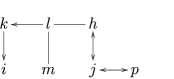
Figure 8: The pairwise Markov property for this RG implies, for example, $\langle i,m\mid\{k,l,h\}\rangle$. The global Markov property would for example imply $\langle\{i,k\},j\mid l\rangle$.

Clearly, the independence model $\mathcal{J}_{m}(G)$ induced by $m$-separation always satisfies the global Markov property w.r.t. $G$. By Lemma 4, Lemma 6, and Theorem 2, $\mathcal{J}_{m}(G)$ satisfies the pairwise Markov property if and only if $G$ is maximal.

6.2 Equivalence of pairwise and global Markov properties

Before establishing the main result of this section, we need two lemmas.

Lemma 8

Let $\mathcal{J}$ be a compositional graphoid over a set $V$ and $M$ and $C$ be disjoint subsets of $V$. It then holds that the marginal independence model

$$\alpha(\mathcal{J},M)=\bigl{\{}\langle A,B\mid C\rangle\colon\ \langle A,B\mid C\rangle\in\mathcal{J}\mbox{ and }(A\cup B\cup C)\cap M=\varnothing\bigr{\}},$$

which is defined over $V\setminus M$, is a compositional graphoid.

[Proof.] All the six compositional graphoid properties for $\alpha(\mathcal{J},M)$ follow trivially from the facts that for $A$, $B$, and $C$ such that $(A\cup B\cup C)\cap M=\varnothing$, $\langle A,B\mid C\rangle\in\alpha(\mathcal{J},M)$ if and only if $\langle A,B\mid C\rangle\in\mathcal{J}$, and $\mathcal{J}$ satisfies the six properties. Notice that the notion of a marginal independence model $\alpha(\mathcal{J},M)$ is identical to the notion formally defined in [24] with a different notation; it was also discussed in [26] with the same notation as in this paper.

The following lemma gives sufficient conditions for the combination of two $m$-connecting paths in anterior graphs to be $m$-connecting.

Lemma 9

Let $G^{*}$ be the anterior graph of a ribbonless graph $G$ and suppose that there are paths $\pi_{1}=\langle i=i_{0},i_{1},\dots,i_{n},h\rangle$ between $i$ and $h$ and $\pi_{2}=\langle h,j_{m},j_{m-1},\dots,j_{0}=j\rangle$ between $h$ and $j$ which are $m$-connecting given $C$. The combination $\pi_{12}=\pi_{1}\circ\pi_{2}$ is then an $m$-connecting path between $i$ and $j$ given $C$ in each of the following mutually exclusive situations:

1. [(b2)]

2. $\langle i_{n},h,j_{m}\rangle$ is a collider and $h\in C\cup\operatorname{an}(C)$;

3. $i_{n}=j_{m}$ with an arrowhead pointing to $h$ on the $i_{n}h$-edge and $h\in C\cup\operatorname{an}(C)$;

4. $\langle i_{n},h,j_{m}\rangle$ is a non-collider and $h\notin C$;

5. $i_{n}=j_{m}$ with no arrowhead pointing to $h$ on the $i_{n}h$-edge.

[Proof.] Let $\pi_{12}=\pi_{1}\circ\pi_{2}=\langle i,\ldots i_{p-1},k,j_{q-1},\dots,j\rangle$ be the combination of $\pi_{1}$ and $\pi_{2}$. If $k=h$ and either (a1) or (b1) holds then the conclusion is obvious. The cases (a2) or (b2) are only relevant when $k\neq h$.

Next consider the situation where $k\neq h$. Since $\pi_{1}$ and $\pi_{2}$ are $m$-connecting, for $\pi_{12}$ to be $m$-connecting we only need to check the tripath $\langle i_{p-1},k,j_{q-1}\rangle$. We have to deal with two cases:

Case 1: $\langle i_{p-1},k,j_{q-1}\rangle$ is a non-collider.

In this case there is no arrowhead pointing to $k$ from at least one of $i_{p-1}$ or $j_{q-1}$. This means that $\langle i_{p-1},k,i_{p+1}\rangle$ on $\pi_{1}$ or $\langle j_{q-1},k,j_{q+1}\rangle$ on $\pi_{2}$ is a non-collider, and since $\pi_{1}$ and $\pi_{2}$ were both $m$-connecting we have $k\notin C$. Hence $\pi_{12}$ is $m$-connecting.

Case 2: $\langle i_{p-1},k,j_{q-1}\rangle$ is a collider. We need to consider the following two subcases:

Case 2.1. If $\langle i_{p-1},k,j_{q-1}\rangle$ is a collider and any of $\langle i_{p-1},k,i_{p+1}\rangle$ or $\langle j_{q-1},k,j_{q+1}\rangle$ is also a collider then $k\in C\cup\operatorname{an}(C)$ and $\pi_{12}$ is $m$-connecting.

Case 2.2. If $\langle i_{p-1},k,j_{q-1}\rangle$ is a collider but $\langle i_{p-1},k,i_{p+1}\rangle$ and $\langle j_{q-1},k,j_{q+1}\rangle$ are both non-colliders then by Lemma 5, the subpath of $\pi_{1}$ from $k$ to a collider node $l_{1}$ or to $h$ is an anterior path and similarly for $\pi_{2}$, $l_{2}$, and $h$. However, since $G^{*}$ is an anterior graph and there are arrowheads pointing to $k$, these anterior paths must be direction-preserving and thus $k\in\operatorname{an}(l_{1})\cup\operatorname{an}(h)$ and $k\in\operatorname{an}(l_{2})\cup\operatorname{an}(h)$. Now we have the two following further subcases:

Case 2.2.1: One of the subpaths of $\pi_{1},\pi_{2}$ from $k$ to $l_{1},l_{2}$ is direction-preserving. Because $\pi_{1}$ and $\pi_{2}$ are $m$-connecting we must have $l_{1}$ or $l_{2}$ in $C\cup\operatorname{an}(C)$. Thus, $k\in\operatorname{an}(C)$ and $\pi_{12}$ is $m$-connecting.

Case 2.2.2: Both subpaths of $\pi_{1}$ and $\pi_{2}$ from $k$ to $h$ are direction-preserving. Then $\langle i_{n},h,j_{m}\rangle$ is collider or $i_{n}=j_{m}$ with an arrowhead pointing to $h$ on the $i_{n}h$-edge and (b1) and (b2) are impossible. If (a1) or (a2) holds $\pi_{12}$ is $m$-connecting since then $h\in C\cup\operatorname{an}(C)$.

We are now ready to establish the main result of this paper.

Theorem 3

Let $G$ be a maximal ribbonless graph. If an independence model $\mathcal{J}$ over the node set of $G$ is a compositional graphoid, then $\mathcal{J}$ satisfies the pairwise Markov property w.r.t. $G$ if and only if it satisfies the global Markov property w.r.t. $G$.

[Proof.] ($\Leftarrow$) If $\mathcal{J}$ is a compositional graphoid and satisfies the global Markov property it follows from Theorem 2 and Lemma 6 that it satisfies the pairwise Markov property.

($\Rightarrow$) Now suppose that $\mathcal{J}$ satisfies the pairwise Markov property and compositional graphoid axioms. For subsets $A$, $B$, and $C$ of the node set of $G$, we should prove that $A\perp_{m}B\mid C$ implies $\langle A,B\mid C\rangle\in\mathcal{J}$. By composition, it is sufficient to show this when $A$ and $B$ are singletons, that is, that $i\perp_{m}j\mid C$ implies $\langle i,j\mid C\rangle\in\mathcal{J}$.

Further we observe that it is sufficient to establish the result in the case when $G=G^{*}$ is itself an anterior graph. Proposition 1 gives that $A\perp_{m}B\mid C$ in $G$, which implies $A\perp_{m}B\mid C$ in $G^{*}$. In addition, by Lemma 7, $G^{*}$ is a maximal graph. Moreover, $G$ and $G^{*}$ have the same anterior sets, and therefore the same pairwise Markov property. Thus in the following, we assume that $G=G^{*}$ is an anterior graph.

We prove the result in two main parts. In part I, we prove the result for the case that $C\subseteq\operatorname{ant}(i)\cup\operatorname{ant}(j)$. In part II, we use the result of part I to establish the general case.

Part I. Suppose that $C\subseteq\operatorname{ant}(i)\cup\operatorname{ant}(j)$. We use induction on the number of nodes of the graph. The induction base for a graph with two nodes is trivial. Thus, suppose that the result holds for all anterior graphs with fewer than $n$ nodes and assume that $G^{*}$ has $n$ nodes.

Let $D=\{i\}\cup\{j\}\cup\operatorname{ant}(i)\cup\operatorname{ant}(j)$ and $M=V\setminus D$, where $V$ is the node set of the graph. First in case I.1 we suppose that $M\neq\varnothing$, and then in case I.2 we suppose that $M=\varnothing$.

Case I.1. Consider $G^{*}[D]$ to be the subgraph induced by $D$. Consider the marginal independence model $\alpha(\mathcal{J},M)=\{\langle A,B\mid C\rangle\colon\ \langle A,B\mid C\rangle\in\mathcal{J}$ and $(A\cup B\cup C)\cap M=\varnothing\}$ defined over $D$. By Lemma 8, $\alpha(\mathcal{J},M)$ is a compositional graphoid. In addition, it satisfies the pairwise Markov property: This is because two non-adjacent nodes $l_{1}$ and $l_{2}$ in $G^{*}[D]$ are non-adjacent in $G^{*}$ and by the pairwise Markov property for $\mathcal{J}$, $\langle l_{1},l_{2}\mid(\operatorname{ant}_{G^{*}}(l_{1})\cup\operatorname{ant}_{G^{*}}(l_{2}))\setminus\{l_{1},l_{2}\}\rangle\in\mathcal{J}$, where $\operatorname{ant}_{G^{*}}$ is the anterior set in $G^{*}$. We know that $\operatorname{ant}_{G^{*}}(l_{1})\cup\operatorname{ant}_{G^{*}}(l_{2})\subseteq D$ and hence $\operatorname{ant}_{G^{*}}(l_{1})\cup\operatorname{ant}_{G^{*}}(l_{2})\cap M=\varnothing$. In addition, for a node $l$ in $G^{*}[D]$, $\operatorname{ant}_{G^{*}}(l)=\operatorname{ant}_{G^{*}[D]}(l)$. Therefore, $\langle l_{1},l_{2}\mid(\operatorname{ant}_{G^{*}[D]}(l_{1})\cup\operatorname{ant}_{G^{*}[D]}(l_{2}))\setminus\{l_{1},l_{2}\}\rangle\in\alpha(\mathcal{J},M)$.

We also know that $i\perp_{m}j\mid C$ in $G^{*}$ implies $i\perp_{m}j\mid C$ in $G^{*}[D]$ since there is no $m$-connecting path between $i$ and $j$ given $C$ in $G^{*}$ and by removing nodes and edges from $G^{*}$ no new $m$-connecting paths are generated. Therefore, by the induction hypothesis $\langle i,j\mid C\rangle\in\alpha(\mathcal{J},M)$. This implies that $\langle i,j\mid C\rangle\in\mathcal{J}$.

Case I.2. Now suppose that $M=\varnothing$ and thus the node set of $G^{*}$ is $D=\{i\}\cup\{j\}\cup\operatorname{ant}(i)\cup\operatorname{ant}(j)$. We prove the result by reverse induction on $|C|$: For the base, $C=V\setminus\{i,j\}=(\operatorname{ant}(i)\cup\operatorname{ant}(j))\setminus\{i,j\}$ and the result follows trivially from the pairwise Markov property.

For the inductive step, consider a node $h\notin C$. We want to show that $h$ is not simultaneously $m$-connected to both $i$ and $j$: Suppose, for contradiction, there are $m$-connecting paths $\pi_{1}=\langle i,i_{1},\dots,i_{n},h\rangle$ and $\pi_{2}=\langle h,j_{m},j_{m-1},\dots,j_{0}=j\rangle$ given $C$. If (b1) or (b2) of Lemma 9 hold then $i$ and $j$ are $m$-connected given $C$ which contradicts $i\perp_{m}j\mid C$. So we need only consider the cases where $\langle i_{n},h,j_{m}\rangle$ is collider or $i_{n}=j_{m}$ with an arrowhead pointing to $h$ on the $i_{n}h$-edge. However, we know that $h\in\operatorname{ant}(i)$ or $h\in\operatorname{ant}(j)$. Because of symmetry between $i$ and $j$ suppose that $h\in\operatorname{ant}(i)$. Since $G^{*}$ is an anterior graph and there is an arrowhead pointing to $h$ we have $h\in\operatorname{an}(i)$. Hence, there is a direction-preserving path $\pi$ from $h$ to $i$. If no node on $\pi$ is in $C$ then (b1) or (b2) of Lemma 9 implies that the combination of $\pi$ and $\pi_{2}$ is an $m$-connecting path between $i$ and $j$, again a contradiction. If there is a node on $\pi$ that is in $C$ then $h\in\operatorname{an}(C)$ and again, by (a1) and (a2) of Lemma 9, $i$ and $j$ are $m$-connected given $C$, again a contradiction.

We conclude that, given $C$, $h$ is not $m$-connected to both $i$ and $j$. By symmetry, suppose that $i\perp_{m}h\mid C$.

We also have that $i\perp_{m}j\mid C$. Since $\mathcal{J}_{m}(G^{*})$ is a compositional graphoid (Theorem 1) the composition property gives that $i\perp_{m}\{j,h\}\mid C$. By weak union for $\perp_{m}$ we obtain $i\perp_{m}j\mid\{h\}\cup C$ and $i\perp_{m}h\mid\{j\}\cup C$. By the induction hypothesis, we obtain $\langle i,j\mid\{h\}\cup C\rangle\in\mathcal{J}$ and $\langle i,h\mid\{j\}\cup C\rangle\in\mathcal{J}$. By intersection, we get $\langle i,\{j,h\}\mid C\rangle\in\mathcal{J}$. By decomposition we finally obtain $\langle i,j\mid C\rangle\in\mathcal{J}$.

Part II. We now prove the result in the general case by induction on $|C|$. The base, that is, the case that $|C|=0$, follows from part I. To prove the inductive step, we can assume that $C\nsubseteq\operatorname{ant}(i)\cup\operatorname{ant}(j)$, since otherwise part I implies the result.

We first show that if $C\nsubseteq\operatorname{ant}(i)\cup\operatorname{ant}(j)$ then there is a node $l$ in $C$ such that $i\perp_{m}j\mid C\setminus\{l\}$: Let first $l^{\prime}\in C\setminus(\operatorname{ant}(i)\cup\operatorname{ant}(j))$ be arbitrary. If there is an $l^{\prime\prime}\in C\setminus(\operatorname{ant}(i)\cup\operatorname{ant}(j))$ so that $l^{\prime}\in\operatorname{ant}(l^{\prime\prime})$ and $l^{\prime\prime}\notin\operatorname{ant}(l^{\prime})$ then replace $l^{\prime}$ by $l^{\prime\prime}$, and repeat this process until it terminates, the latter being ensured by transitivity of $\operatorname{ant}$ (Lemma 1) and the finiteness of $C$. Thus, we eventually obtain an $l$ so that if $l\in\operatorname{ant}(\tilde{l})$ for $\tilde{l}\in C\setminus(\operatorname{ant}(i)\cup\operatorname{ant}(j))$ then we also have $\tilde{l}\in\operatorname{ant}(l)$.

Suppose, for contradiction, that there is a shortest $m$-connecting path $\pi$ between $i$ and $j$ given $C\setminus\{l\}$. If $l$ is not on $\pi$ or is a collider on $\pi$ then $\pi$ is also $m$-connecting given $C$. Therefore, $l$ is a non-collider on $\pi$. This, together with $l\notin\operatorname{ant}(i)\cup\operatorname{ant}(j)$, by using Lemma 5, implies that $l$ is an anterior of a collider node $p$ on $\pi$. Since $\pi$ is $m$-connecting, $p\in C\cup\operatorname{an}(C)$. Thus, there is an $\tilde{l}\in C$ so that $p=\tilde{l}$ or $p\in\operatorname{an}(\tilde{l})$. Transitivity of anterior sets and the fact that $l\notin(\operatorname{ant}(i)\cup\operatorname{ant}(j))$ now imply that $\tilde{l}\in C\setminus(\operatorname{ant}(i)\cup\operatorname{ant}(j))$. The construction of $l$ implies $\tilde{l}\in\operatorname{ant}(l)$ which again implies that $\tilde{l}\in\operatorname{an}(l)$ and $l\in\operatorname{an}(\tilde{l})$ and thus the collider tripath containing $p$ is a cyclic ribbon unless its endpoints are adjacent with an endpoint-identical edge, which implies that $\pi$ is not a shortest $m$-connecting path, a contradiction.

We now have that either $i\perp_{m}l\mid C\setminus\{l\}$ or $j\perp_{m}l\mid C\setminus\{l\}$ since otherwise, by Lemma 9 there is an $m$-connecting path between $i$ and $j$ given $C\setminus\{l\}$ in the case that $l$ is a non-collider or given $C$ in the case that $l$ is a collider node. Because of symmetry suppose that $i\perp_{m}l\mid C\setminus\{l\}$. By the induction hypothesis, we have $\langle i,j\mid C\setminus\{l\}\rangle\in\mathcal{J}$ and $\langle i,l\mid C\setminus\{l\}\rangle\in\mathcal{J}$. By the composition property we get $\langle i,\{j,l\}\mid C\setminus\{l\}\rangle\in\mathcal{J}$. The weak union property implies $\langle i,j\mid C\rangle\in\mathcal{J}$. If we specialise Theorem 3 to the most common case of probabilistic independence models, we get the following corollary.

Corollary 2

Let $G$ be a maximal ribbonless graph. A probabilistic independence model that satisfies the intersection and composition axioms satisfies the pairwise Markov property w.r.t. $G$ if and only if it satisfies the global Markov property w.r.t. $G$.

6.3 Necessity of compositional graphoid axioms

Theorem 3 states that, for equivalence of pairwise and global Markov properties, the six compositional graphoid axioms are sufficient. In fact, in general, for the mentioned equivalence, all six axioms are also necessary. The graphs in Figure 9 show that the intersection and composition properties are necessary for the equivalence of pairwise and global Markov properties.

For $G_{1}=(V_{1},E_{1})$, if $\mathcal{J}_{1}$ defined over $V_{1}$ satisfies the pairwise Markov property, then $\langle i,k\mid\{j,l\}\rangle$, $\langle i,l\mid\{j,k\}\rangle$, and $\langle k,l\mid\{i,j\}\rangle$ are in $\mathcal{J}_{1}$. It can be seen that none of the compositional semi-graphoid axioms can be used to imply $\langle i,\{k,l\}\mid j\rangle\in\mathcal{J}_{1}$. The intersection property is the only axiom that implies the result.

For $G_{2}=(V_{2},E_{2})$, if $\mathcal{J}_{2}$ defined over $V_{2}$ satisfies the pairwise Markov property then $\langle i,k\mid\varnothing\rangle$, $\langle i,l\mid\varnothing\rangle$, and $\langle k,l\mid\varnothing\rangle$ are in $\mathcal{J}_{2}$. It can be seen that none of the graphoid axioms can be used to imply $\langle i,\{k,l\}\mid\varnothing\rangle\in\mathcal{J}_{2}$. The composition property is the only axiom that implies the result.

For $G_{3}=(V_{3},E_{3})$, if $\mathcal{J}_{3}$ defined over $V_{3}$ satisfies the pairwise Markov property then $\langle i,k\mid\varnothing\rangle$, $\langle i,l\mid\{j,k\}\rangle$, and $\langle k,l\mid\{i,j\}\rangle$ are in $\mathcal{J}_{3}$. It can be seen that none of the compositional semi-graphoid axioms can be used to imply $\langle l,\{i,k\}\mid j\rangle\in\mathcal{J}_{3}$. The intersection property is the only axiom that implies the result. See also for example, Example 3.26 of [19], showing that the pairwise Markov property does not imply the global Markov property for DAGs when intersection is violated.

Figure 9: For the equivalence of pairwise and global Markov properties, (a) an undirected graph $G_{1}$ that shows that the intersection property is necessary; (b) a bidirected graph $G_{2}$ that shows that the composition property is necessary; (c) a directed acyclic graph $G_{3}$ that shows that the intersection property is necessary.

It is known that, for undirected graphs, the five graphoid axioms are necessary and sufficient for equivalence of pairwise and global Markov properties; see [19]. For bidirected graphs, the independence statement associated with a missing edge between nodes $i$ and $j$ is $\langle i,j\mid\varnothing\rangle$ and only the five compositional semi-graphoid axioms are necessary for equivalence of pairwise and global Markov properties. This can be inferred from the proof of Theorem 3, since part I of the proof is not relevant for bidirected graphs unless $C=\varnothing$ and the intersection property is not used in part II of the proof. We conclude by stating this as its own proposition.

Proposition 0

Let $G=(V,E)$ be a bidirected graph. If an independence model $\mathcal{J}$ defined over $V$ is a compositional semi-graphoid then $\mathcal{J}$ satisfies the pairwise Markov property w.r.t. $G$ if and only if it satisfies the global Markov property w.r.t. $G$.

References

- [1] {barticle}[mr] \bauthor\bsnmAndersson, \bfnmSteen A.\binitsS.A., \bauthor\bsnmMadigan, \bfnmDavid\binitsD. &\bauthor\bsnmPerlman, \bfnmMichael D.\binitsM.D. (\byear1997). \btitleA characterization of Markov equivalence classes for acyclic digraphs. \bjournalAnn. Statist. \bvolume25 \bpages505–541. \biddoi=10.1214/aos/1031833662, issn=0090-5364, mr=1439312\bptokimsref\endbibitem
- [2] {barticle}[mr] \bauthor\bsnmAndersson, \bfnmSteen A.\binitsS.A., \bauthor\bsnmMadigan, \bfnmDavid\binitsD. &\bauthor\bsnmPerlman, \bfnmMichael D.\binitsM.D. (\byear2001). \btitleAlternative Markov properties for chain graphs. \bjournalScand. J. Statist. \bvolume28 \bpages33–85. \biddoi=10.1111/1467-9469.00224, issn=0303-6898, mr=1844349 \bptokimsref\endbibitem
- [3] {barticle}[mr] \bauthor\bsnmBesag, \bfnmJulian\binitsJ. (\byear1974). \btitleSpatial interaction and the statistical analysis of lattice systems. \bjournalJ. Roy. Statist. Soc. Ser. B \bvolume36 \bpages192–236. \bnoteWith discussion by D.R. Cox, A.G. Hawkes, P. Clifford, P. Whittle, K. Ord, R. Mead, J.M. Hammersley and M.S. Bartlett and with a reply by the author. \bidissn=0035-9246, mr=0373208 \bptnotecheck related \bptokimsref\endbibitem
- [4] {bincollection}[mr] \bauthor\bsnmClifford, \bfnmPeter\binitsP. (\byear1990). \btitleMarkov random fields in statistics. In \bbooktitleDisorder in Physical Systems. \bseriesOxford Sci. Publ. \bpages19–32. \blocationNew York: \bpublisherOxford Univ. Press. \bidmr=1064553 \bptokimsref\endbibitem
- [5] {barticle}[mr] \bauthor\bsnmCox, \bfnmD. R.\binitsD.R. &\bauthor\bsnmWermuth, \bfnmNanny\binitsN. (\byear1993). \btitleLinear dependencies represented by chain graphs. \bjournalStatist. Sci. \bvolume8 \bpages204–218, 247–283. \bnoteWith comments and a rejoinder by the authors. \bidissn=0883-4237, mr=1243593 \bptnotecheck related \bptokimsref\endbibitem
- [6] {barticle}[mr] \bauthor\bsnmDarroch, \bfnmJ. N.\binitsJ.N., \bauthor\bsnmLauritzen, \bfnmS. L.\binitsS.L. &\bauthor\bsnmSpeed, \bfnmT. P.\binitsT.P. (\byear1980). \btitleMarkov fields and log-linear interaction models for contingency tables. \bjournalAnn. Statist. \bvolume8 \bpages522–539. \bidissn=0090-5364, mr=0568718 \bptokimsref\endbibitem
- [7] {barticle}[mr] \bauthor\bsnmDawid, \bfnmA. P.\binitsA.P. (\byear1979). \btitleConditional independence in statistical theory. \bjournalJ. Roy. Statist. Soc. Ser. B \bvolume41 \bpages1–31. \bidissn=0035-9246, mr=0535541 \bptnotecheck related \bptokimsref\endbibitem
- [8] {barticle}[mr] \bauthor\bsnmDrton, \bfnmMathias\binitsM. (\byear2009). \btitleDiscrete chain graph models. \bjournalBernoulli \bvolume15 \bpages736–753. \biddoi=10.3150/08-BEJ172, issn=1350-7265, mr=2555197 \bptokimsref\endbibitem
- [9] {barticle}[mr] \bauthor\bsnmDrton, \bfnmMathias\binitsM. &\bauthor\bsnmRichardson, \bfnmThomas S.\binitsT.S. (\byear2008). \btitleBinary models for marginal independence. \bjournalJ. R. Stat. Soc. Ser. B Stat. Methodol. \bvolume70 \bpages287–309. \biddoi=10.1111/j.1467-9868.2007.00636.x, issn=1369-7412, mr=2424754 \bptokimsref\endbibitem
- [10] {barticle}[mr] \bauthor\bsnmFrydenberg, \bfnmMorten\binitsM. (\byear1990). \btitleThe chain graph Markov property. \bjournalScand. J. Statist. \bvolume17 \bpages333–353. \bidissn=0303-6898, mr=1096723 \bptokimsref\endbibitem
- [11] {barticle}[mr] \bauthor\bsnmGeiger, \bfnmDan\binitsD., \bauthor\bsnmVerma, \bfnmThomas\binitsT. &\bauthor\bsnmPearl, \bfnmJudea\binitsJ. (\byear1990). \btitleIdentifying independence in Bayesian networks. \bjournalNetworks \bvolume20 \bpages507–534. \biddoi=10.1002/net.3230200504, issn=0028-3045, mr=1064736 \bptokimsref\endbibitem
- [12] {barticle}[mr] \bauthor\bsnmGrimmett, \bfnmG. R.\binitsG.R. (\byear1973). \btitleA theorem about random fields. \bjournalBull. London Math. Soc. \bvolume5 \bpages81–84. \bidissn=0024-6093, mr=0329039 \bptokimsref\endbibitem
- [13] {bmisc}[auto:STB—2013/01/29—08:09:18] \bauthor\bsnmHammersley, \bfnmJ. M.\binitsJ.M. &\bauthor\bsnmClifford, \bfnmP.\binitsP. (\byear1971) \bhowpublishedMarkov fields on finite graphs and lattices. Unpublished manuscript. \bptokimsref\endbibitem
- [14] {barticle}[auto:STB—2013/01/29—08:09:18] \bauthor\bsnmKang, \bfnmC.\binitsC. &\bauthor\bsnmTian, \bfnmJ.\binitsJ. (\byear2009). \btitleMarkov properties for linear causal models with correlated errors. \bjournalJ. Mach. Learn. Res. \bvolume10 \bpages41–70. \bptokimsref\endbibitem
- [15] {barticle}[mr] \bauthor\bsnmKauermann, \bfnmGöran\binitsG. (\byear1996). \btitleOn a dualization of graphical Gaussian models. \bjournalScand. J. Statist. \bvolume23 \bpages105–116. \bidissn=0303-6898, mr=1380485 \bptokimsref\endbibitem
- [16] {barticle}[mr] \bauthor\bsnmKiiveri, \bfnmHarri\binitsH., \bauthor\bsnmSpeed, \bfnmT. P.\binitsT.P. &\bauthor\bsnmCarlin, \bfnmJ. B.\binitsJ.B. (\byear1984). \btitleRecursive causal models. \bjournalJ. Austral. Math. Soc. Ser. A \bvolume36 \bpages30–52. \bidissn=0263-6115, mr=0719999 \bptokimsref\endbibitem
- [17] {barticle}[mr] \bauthor\bsnmKoster, \bfnmJan T. A.\binitsJ.T.A. (\byear1997). \btitleGibbs and Markov properties of graphs. \bjournalAnn. Math. Artificial Intelligence \bvolume21 \bpages13–26. \biddoi=10.1023/A:1018948915264, issn=1012-2443, mr=1479006 \bptokimsref\endbibitem
- [18] {barticle}[mr] \bauthor\bsnmKoster, \bfnmJan T. A.\binitsJ.T.A. (\byear2002). \btitleMarginalizing and conditioning in graphical models. \bjournalBernoulli \bvolume8 \bpages817–840. \bidissn=1350-7265, mr=1963663 \bptokimsref\endbibitem
- [19] {bbook}[mr] \bauthor\bsnmLauritzen, \bfnmSteffen L.\binitsS.L. (\byear1996). \btitleGraphical Models. \bseriesOxford Statistical Science Series \bvolume17. \blocationNew York: \bpublisherClarendon Press. \bidmr=1419991 \bptokimsref\endbibitem
- [20] {barticle}[mr] \bauthor\bsnmLauritzen, \bfnmSteffen L.\binitsS.L. &\bauthor\bsnmRichardson, \bfnmThomas S.\binitsT.S. (\byear2002). \btitleChain graph models and their causal interpretations. \bjournalJ. R. Stat. Soc. Ser. B Stat. Methodol. \bvolume64 \bpages321–361. \biddoi=10.1111/1467-9868.00340, issn=1369-7412, mr=1924296 \bptnotecheck related \bptokimsref\endbibitem
- [21] {bbook}[mr] \bauthor\bsnmPearl, \bfnmJudea\binitsJ. (\byear1988). \btitleProbabilistic Reasoning in Intelligent Systems: Networks of Plausible Inference. \bseriesThe Morgan Kaufmann Series in Representation and Reasoning. \blocationSan Mateo, CA: \bpublisherMorgan Kaufmann. \bidmr=0965765 \bptokimsref\endbibitem
- [22] {bmisc}[auto:STB—2013/01/29—08:09:18] \bauthor\bsnmRichardson, \bfnmT.\binitsT. (\byear2001) \bhowpublishedChain graphs which are maximal ancestral graphs are recursive causal graphs. Technical Report 387, Dept. Statistics, Univ. Washington, Seattle, WA. \bptokimsref\endbibitem
- [23] {barticle}[mr] \bauthor\bsnmRichardson, \bfnmThomas\binitsT. (\byear2003). \btitleMarkov properties for acyclic directed mixed graphs. \bjournalScand. J. Statist. \bvolume30 \bpages145–157. \biddoi=10.1111/1467-9469.00323, issn=0303-6898, mr=1963898 \bptokimsref\endbibitem
- [24] {barticle}[mr] \bauthor\bsnmRichardson, \bfnmThomas\binitsT. &\bauthor\bsnmSpirtes, \bfnmPeter\binitsP. (\byear2002). \btitleAncestral graph Markov models. \bjournalAnn. Statist. \bvolume30 \bpages962–1030. \biddoi=10.1214/aos/1031689015, issn=0090-5364, mr=1926166 \bptokimsref\endbibitem
- [25] {bincollection}[auto:STB—2013/01/29—08:09:18] \bauthor\bsnmRichardson, \bfnmT. S.\binitsT.S. (\byear1998). \btitleChain graphs and symmetric associations. In \bbooktitleLearning in Graphical Models (\beditor\bfnmM.\binitsM. \bsnmJordan, ed.) \bpages231–260. \blocationDordrecht, The Netherlands: \bpublisherKluwer. \bptokimsref\endbibitem
- [26] {bmisc}[auto:STB—2013/01/29—08:09:18] \bauthor\bsnmSadeghi, \bfnmK.\binitsK. \bhowpublished(2013). Stable mixed graphs. Bernoulli 19 2330–2358. \bptokimsref\endbibitem
- [27] {bmisc}[auto:STB—2013/01/29—08:09:18] \bauthor\bsnmSadeghi, \bfnmK.\binitsK. (\byear2012). \btitleGraphical representation of independence structures. \bhowpublishedPh.D. thesis, Univ. Oxford. \bptokimsref\endbibitem
- [28] {bmisc}[auto:STB—2013/01/29—08:09:18] \bauthor\bsnmSpirtes, \bfnmP.\binitsP., \bauthor\bsnmRichardson, \bfnmT.\binitsT. &\bauthor\bsnmMeek, \bfnmC.\binitsC. \bhowpublished(1997). The dimensionality of mixed ancestral graphs. Technical Report CMU-PHIL-83, Dept. Philosophy, Carnegie–Mellon Univ., Pittsburgh, PA. \bptokimsref\endbibitem
- [29] {barticle}[mr] \bauthor\bsnmStudený, \bfnmM.\binitsM. (\byear1989). \btitleMulti-information and the problem of characterization of conditional independence relations. \bjournalProblems Control Inform. Theory/Problemy Upravlen. Teor. Inform. \bvolume18 \bpages3–16. \bidissn=0370-2529, mr=0986211 \bptokimsref\endbibitem
- [30] {barticle}[mr] \bauthor\bsnmWermuth, \bfnmNanny\binitsN. (\byear2011). \btitleProbability distributions with summary graph structure. \bjournalBernoulli \bvolume17 \bpages845–879. \biddoi=10.3150/10-BEJ309, issn=1350-7265, mr=2817608 \bptokimsref\endbibitem
- [31] {barticle}[mr] \bauthor\bsnmWermuth, \bfnmNanny\binitsN. &\bauthor\bsnmCox, \bfnmDavid R.\binitsD.R. (\byear1998). \btitleOn association models defined over independence graphs. \bjournalBernoulli \bvolume4 \bpages477–495. \biddoi=10.2307/3318662, issn=1350-7265, mr=1679794 \bptokimsref\endbibitem
- [32] {barticle}[mr] \bauthor\bsnmWermuth, \bfnmNanny\binitsN., \bauthor\bsnmMarchetti, \bfnmGiovanni M.\binitsG.M. &\bauthor\bsnmCox, \bfnmD. R.\binitsD.R. (\byear2009). \btitleTriangular systems for symmetric binary variables. \bjournalElectron. J. Stat. \bvolume3 \bpages932–955. \biddoi=10.1214/09-EJS439, issn=1935-7524, mr=2540847 \bptokimsref\endbibitem