The generalized Gibbs ensemble as a pseudo-initial state: its predictive power revealed in a second quench

Abstract

The generalized Gibbs ensemble has been shown to be relevant in the relaxation of a completely integrable system subject to a quantum quench, in the sense that it accurately predicts the steady values of some physical variables. We proceed to further question its relevance by giving the quenched system a second quench. The concern is whether the generalized Gibbs ensemble can also accurately predict the relaxed system’s response to the second quench. Two case studies with the transverse Ising model and the hard-core bosons in one dimension yield an affirmative answer. The relevance of the generalized Gibbs ensemble in the non-equilibrium dynamics of integrable systems is then greatly strengthened.

Recently, non-equilibrium dynamics of many-body systems has attracted a lot of attention Polkovnikov . One common concern is whether an initially out-of-equilibrium system can thermalize to behave like a textbook Gibbs ensemble, and how integrability notion ; weiss or non-integrability of the system will affect its relaxation dynamics. An important achievement on this issue is identification of the relevance of the generalized Gibbs ensemble (GGE) in the relaxation dynamics of a completely integrable system rigol07 . The so called generalized Gibbs ensemble is constructed according to the principle of maximum entropy jaynes while taking into account all the constants of motion, whose values are determined by the initial state. With the same philosophy behind the construction, it is a natural counterpart of the usual Gibbs ensembles for a non-integrable system. So far, the GGE has been found to predict correctly the asymptotic values of physical variables in a variety of integrable systems Polkovnikov ; cardy07 ; rigol07 ; cazalilla ; kollar08 ; Calabrese11 ; mussardo ; caneva ; cazalilla11 ; limitation .

The fact that asymptotically, the true, constantly evolving system agrees well with the GGE on the physical quantities is definitely a non-trivial and pleasant one. However, one should not be content with this fact only. Our daily experience in the (mostly non-integrable) macroscopic world is that, if a system relaxes to some steady state, it relaxes in the sense that not only its static properties (i.e. values of the physical quantities) but also its dynamical properties agree with the steady state. To be specific, the system should respond to later perturbations as if it were indeed in the steady state. Therefore, it is necessary to check whether the GGE has this merit. If so, it surely adds to the relevance of the GGE in the non-equilibrium dynamics of a completely integrable system. It would mean that the true system is hardly distinguishable from the GGE neither by static nor dynamical criterions, and it would be fair to say the system has thermalized as much as possible.

Motivated by this problem, we have studied the transverse Ising model and the hard-core bosons in one-dimension (which can also be mapped to the XX model) individually. The two models are integrable and both have been shown to admit a GGE account of their asymptotic behaviors after a quantum quench. Here our idea is to give them a second quench when they have reached the steady phase zjm . The concern is whether they will respond as if the systems were in the GGE states. The result turns out to be the case.

Transverse Ising model.—The Hamiltonian of the model is $H(g)=-\sum_{l=1}^{N}\left(\sigma_{l}^{x}\sigma_{l+1}^{x}-g\sigma_{l}^{z}\right)$, where $\sigma_{l}^{x,z}$ are Pauli matrices acting on a $1/2$-spin at site $l$. Here periodic boundary condition is assumed and $N$ is an even integer large enough. Below, quenches of the system correspond to changing the value of $g$ (strength of the transverse magnetic field) suddenly. We will consider a double quench scenario. Initially the value of $g$ is $g_{0}$ and the system is in its ground state $|G_{0}\rangle$. Then the value of $g$ is changed successively to $g_{1}$ and $g_{2}$.

Under the Jordan-Wigner transform $(\sigma_{l}^{x}+i\sigma_{l}^{y},\sigma_{l}^{x}-i\sigma_{l}^{y})/2=(a_{l}^{\dagger},a_{l})\exp(-i\pi\sum_{r=1}^{l-1}a_{r}^{\dagger}a_{r})$, $\sigma_{l}^{z}=2a_{l}^{\dagger}a_{l}-1$, where $a_{l}^{\dagger}$ and $a_{l}$ are fermionic operators, the Hamiltonian is rewritten as $H(g)=-\sum_{l=1}^{N}[\left(a_{l}^{+}a_{l+1}^{+}+a_{l}^{+}a_{l+1}+h.c.\right)-2ga_{l}^{\dagger}a_{l}]$, with a constant term dropped lieb . Note that here the boundary condition is anti-periodic supple . Taking the Fourier transform $b_{k}=\frac{1}{\sqrt{N}}\sum_{l}e^{i2\pi kl/N}a_{l}$, with $k=-N/2+1/2,\cdots,-1/2,1/2,\cdots,N/2-1/2$ so as to comply with the anti-periodic boundary condition, we can rewrite the Hamiltonian as ($\phi_{k}=2\pi k/N$)

$$H(g)=\sum_{k}\left[2(g-\cos\phi_{k})b_{k}^{\dagger}b_{k}-i\sin\phi_{k}(b_{-k}b_{k}+b_{-k}^{\dagger}b_{k}^{\dagger})\right].$$

It is ready to verify that $b_{k}$ and $b_{-k}^{\dagger}$ are coupled in their equations of motion and this suggests the Bogoliubov transformation $\eta_{k}=u_{k}b_{k}+iv_{k}b_{-k}^{\dagger}$. With $\varepsilon_{k}=2\sqrt{1+g^{2}-2g\cos\phi_{k}}\geq 0$, $(\cos\theta_{k},\sin\theta_{k})=2(g-\cos\phi_{k},\sin\phi_{k})/\varepsilon_{k}$, and $(u_{k},v_{k})=(\cos\frac{\theta_{k}}{2},\sin\frac{\theta_{k}}{2})$, the Hamiltonian is finally diagonalized as $H=\sum_{k}\varepsilon_{k}\eta_{k}^{\dagger}\eta_{k}$. Here again the constant term is dropped. Note that $u_{k}$, $v_{k}$, $\theta_{k}$, and $\varepsilon_{k}$ all depend on $g$. The dependence will be displayed explicitly when necessary.

We are interested in the correlation functions $\langle\sigma_{i}^{x}\sigma_{j}^{x}\rangle$, $\langle\sigma_{i}^{z}\sigma_{j}^{z}\rangle$, and the transverse magnetization $\langle M_{z}\rangle\equiv\langle\sum_{l}\sigma_{l}^{z}\rangle=\langle\sum_{k}(2b_{k}^{\dagger}b_{k}-1)\rangle$. Here the expectation values may be taken with respect to various states as shown below. Introducing $A_{l}=a_{l}^{\dagger}+a_{l}$ and $B_{l}=a_{l}^{\dagger}-a_{l}$, we can rewrite them as $\langle\sigma_{i}^{x}\sigma_{j}^{x}\rangle=\langle B_{i}A_{i+1}B_{i+1}\cdots A_{j-1}B_{j-1}A_{j}\rangle$ and $\langle\sigma_{i}^{z}\sigma_{j}^{z}\rangle=\langle B_{i}A_{i}B_{j}A_{j}\rangle$ lieb . These forms allow us to use Wick’s theorem to do the calculation. The correlation functions will be decomposed into sums of products of the basic correlators $\langle A_{l}A_{m}\rangle$, $\langle B_{l}B_{m}\rangle$, and $\langle B_{l}A_{m}\rangle$.

The initial state $|G_{0}\rangle$ is defined as $\eta_{k}(g_{0})|G_{0}\rangle=0$ for all $k$, or explicitly, $|G_{0}\rangle\propto\prod_{k}\eta_{k}(g_{0})|\psi\rangle$ where $|\psi\rangle$ can be an arbitrary state as long as $\eta_{k}(g_{0})|\psi\rangle\neq 0$. After the first quench of changing $g$ from $g_{0}$ to $g_{1}$ at $t=0$, we have $\langle G_{0}|A_{l}(t)A_{m}(t)|G_{0}\rangle\rightarrow\delta_{lm}$ for $t$ large enough recurrence ; sengupta , and similarly $\langle G_{0}|B_{l}(t)B_{m}(t)|G_{0}\rangle\rightarrow-\delta_{lm}$ for $t$ large enough. But $\langle G_{0}|B_{l}(t)A_{m}(t)|G_{0}\rangle\rightarrow G_{l,m}^{(1)}$, which has the value of

$$G_{l,m}^{(1)}=-\frac{1}{N}\sum_{k}e^{i\phi_{k}(m-l)+i\theta_{k}(g_{1})}\cos(\Delta\theta_{k}^{10}).$$ (1)

Here and hereafter $\Delta\theta_{k}^{ij}\equiv\theta_{k}(g_{i})-\theta_{k}(g_{j})$. Thus for $t$ large enough, $\langle G_{0}|\sigma_{i}^{x}(t)\sigma_{j}^{x}(t)|G_{0}\rangle\rightarrow C_{ij}^{x}$:

$$C_{ij}^{x}=\text{Det}\left(\begin{array}[]{cccc}G_{i,i+1}^{(1)}&G_{i,i+2}^{(1)}&\cdots&G_{i,j}^{(1)}\\ G_{i+1,i+1}^{(1)}&G_{i+1,i+2}^{(1)}&\cdots&G_{i+1,j}^{(1)}\\ \cdots&\cdots&\cdots&\cdots\\ G_{j-1,i+1}^{(1)}&G_{j-1,i+2}^{(1)}&\cdots&G_{j-1,j}^{(1)}\end{array}\right),$$ (2)

and

$$\langle G_{0}|\sigma_{i}^{z}(t)\sigma_{j}^{z}(t)|G_{0}\rangle\rightarrow C_{ij}^{z}=G_{i,i}^{(1)}G_{j,j}^{(1)}-G_{i,j}^{(1)}G_{j,i}^{(1)}.$$ (3)

As for the transverse magnetization, $\langle\Psi_{0}|M_{z}(t)|\Psi_{0}\rangle$ has the asymptotic value of

$$M_{z}^{(1)}=-\sum_{k}\cos\theta_{k}(g_{1})\cos(\Delta\theta_{k}^{10}).$$ (4)

On the other hand, from $g_{0}$ to $g_{1}$, the (first) GGE density matrix is defined as

$$\rho_{gge1}=\frac{1}{Z_{1}}\prod_{k}\exp\left(-\lambda_{k}^{(1)}\eta_{k}^{\dagger}(g_{1})\eta_{k}(g_{1})\right),$$ (5)

with the Lagrange multiplier $\lambda_{k}^{(1)}$ determined by the condition $\langle G_{0}|\eta_{k}^{\dagger}(g_{1})\eta_{k}(g_{1})|G_{0}\rangle=tr(\eta_{k}^{\dagger}(g_{1})\eta_{k}(g_{1})\rho_{gge1})$, and $Z_{1}=\prod_{k}(1+e^{-\lambda_{k}^{(1)}})$. It can be verified that $\langle A_{l}A_{m}\rangle_{gge1}=-\langle B_{l}B_{m}\rangle_{gge1}=\delta_{lm}$, and $\langle B_{l}A_{m}\rangle_{gge1}=G_{l,m}^{(1)}$. Here the subscript means averaging over $\rho_{gge1}$. Thus the basic correlators are of the same values with respect to the GGE density matrix $\rho_{gge1}$ and the evolving state $e^{-iH(g_{1})t}|G_{0}\rangle$ for $t$ large enough. This fact then indicates that the asymptotic values of the correlation functions (2) and (3) can be recovered with the GGE. Likewise, the asymptotic value of the transverse magnetization (4) is exactly predicted by the GGE, i.e., $M_{z}^{(1)}=tr(M_{z}\rho_{gge1})$ Polkovnikov ; supple .

Now consider giving the system a second quench, i.e., changing the value of $g$ from $g_{1}$ to $g_{2}$ at some time $t=t_{1}$. It is tedious but straightforward to show that at the time of $t=t_{1}+t_{2}$, for large $t_{2}$ supple , $\langle G_{0}|A_{l}(t)A_{m}(t)|G_{0}\rangle\simeq\delta_{lm}+$oscillating terms depending on $t_{1}$, and similarly $\langle G_{0}|B_{l}(t)B_{m}(t)|G_{0}\rangle\simeq-\delta_{lm}+$oscillating terms depending on $t_{1}$. However, $\langle G_{0}|B_{l}(t)A_{m}(t)|G_{0}\rangle\simeq G_{l,m}^{(2)}+$oscillating terms depending on $t_{1}$, where

$$G_{l,m}^{(2)}=-\frac{1}{N}\sum_{k}e^{i\phi_{k}(m-l)+i\theta_{k}(g_{2})}\cos(\Delta\theta_{k}^{10})\cos(\Delta\theta_{k}^{21}).$$ (6)

As for the transverse magnetization, $\langle G_{0}|M_{z}(t)|G_{0}\rangle\rightarrow M_{z}^{(2)}+$oscillating terms depending on $t_{1}$, with

$$M_{z}^{(2)}=-\sum_{k}\cos\theta_{k}(g_{2})\cos(\Delta\theta_{k}^{10})\cos(\Delta\theta_{k}^{21}).$$ (7)

The oscillating terms depending on $t_{1}$ consist of $O(N)$ components of different non-zero frequencies and thus they virtually vanish for $t_{1}$ large enough. Therefore, for $t_{1}$ and $t_{2}$ large enough, the correlation functions $\langle G_{0}|\sigma_{i}^{x}(t)\sigma_{j}^{x}(t)|G_{0}\rangle$ and $\langle G_{0}|\sigma_{i}^{z}(t)\sigma_{j}^{z}(t)|G_{0}\rangle$ have the same form as Eqs. (2) and (3) but with $G_{m,l}^{(1)}$ replaced by $G_{m,l}^{(2)}$, and $\langle G_{0}|M_{z}(t)|G_{0}\rangle$ has the value of $M_{z}^{(2)}$.

On the other hand, if the second quench is imposed on the first GGE density matrix $\rho_{gge1}$, we have the same asymptotic behaviors of the basic correlators and the transverse magnetization for large $t_{2}$. That is, $\langle A_{l}(t_{2})A_{m}(t_{2})\rangle=-\langle B_{l}(t_{2})B_{m}(t_{2})\rangle\simeq\delta_{lm}$, $\langle B_{m}(t_{2})A_{l}(t_{2})\rangle\simeq G_{m,l}^{(2)}$, and $\langle M_{z}(t_{2})\rangle\simeq M_{z}^{(2)}$ supple . Here $(A_{l}(t_{2}),B_{l}(t_{2}),M_{z}(t_{2}))=e^{iH(g_{2})t_{2}}(A_{l},B_{l},M_{z})e^{-iH(g_{2})t_{2}}$ and the average is taken over $\rho_{gge1}$. We see that the transverse magnetization as well as the basic correlators possess the same asymptotic values regardless of the initial state being $e^{-iH(g_{1})t_{1}}|G_{0}\rangle$ or $\rho_{gge1}$. The latter fact implies that the correlation functions have the same property. However, it is not only the asymptotic values that can be accurately reproduced by using $\rho_{gge1}$ as a substitute for $e^{-iH(g_{1})t_{1}}|G_{0}\rangle$. In Fig. 1, the transient dynamics of $M_{z}$ after the second quench is shown. There we see that as long as $t_{1}$ is large enough, the relaxation dynamics of $M_{z}$ (the correlation functions have the same property; see the supplementary material) is independent of $t_{1}$ and can be reproduced by $\rho_{gge1}$ even to minute details. Therefore, as long as $t_{1}$ is large enough, or as long as the second quench comes when the system has equilibrated to agree with the first GGE $\rho_{gge1}$ after the first quench, the model reacts as if it were indeed in the GGE state $\rho_{gge1}$. That is, the GGE density matrix $\rho_{gge1}$ can serve as a pseudo-initial state to the second quench.

Finally, for the quench of $\rho_{gge1}$, we can define a second GGE density matrix as

$$\rho_{gge2}=\frac{1}{Z_{2}}\prod_{k}\exp\left(-\lambda_{k}^{(2)}\eta_{k}^{\dagger}(g_{2})\eta_{k}(g_{2})\right),$$ (8)

with the parameter $\lambda_{k}^{(2)}$ determined by the condition $tr(\eta_{k}^{\dagger}(g_{2})\eta_{k}(g_{2})\rho_{gge2})=tr(\eta_{k}^{\dagger}(g_{2})\eta_{k}(g_{2})\rho_{gge1})$, and $Z_{2}=\prod_{k}(1+e^{-\lambda_{k}^{(2)}})$. The point is that the basic correlator $G_{l,m}^{(2)}$ in (6) and the transverse magnetization in (7) can be exactly reproduced by $\rho_{gge2}$. This is one more support of the argument that $\rho_{gge1}$ can serve as a pseudo-initial state to the second quench.

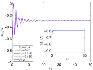
Figure 1: (Color online) Evolution of the transverse magnetization $M_{z}$ after the second quench. The parameters are $(N,g_{0},g_{1},g_{2})=(10000,2,1,0.2)$. All the lines, with the “initial” state being the (first) generalized Gibbs ensemble (GGE) density matrix $\rho_{gge1}$ or $e^{-iH(g_{1})t_{1}}|G_{0}\rangle$, collapse into one. Here the values of $t_{1}$ are chosen randomly from $[500,2500]$. The horizontal dotted line indicates the predicted asymptotic value (7). The insert shows the time evolution of $M_{z}$ after the first quench.

Expansion of hard-core bosons in a one dimensional lattice.—To make contact with previous works, the scenario studied below is an extension of that in Ref. rigol07 . There are $N$ hard-core bosons and there is a lattice of $M_{2}$ sites, which are numbered from $1$ to $M_{2}$. Initially the $N$ bosons are confined to the $M_{0}$ middle sites by hard-walls on the two sides and the system is in the ground state, which is denoted as $\psi_{0}$. At $t=0$, the hard-walls are suddenly moved outward symmetrically so that now $M_{1}$ sites are contained. The system then evolves and as found by Rigol et al. rigol07 , the GGE plays an important role in the ensuing dynamics—the momentum distribution of the bosons in its steady value is accurately captured by the GGE density matrix $\Xi_{gge1}$ (see below). Our idea is then at some time $t_{1}$, when the momentum distribution has settled down to its steady value, to increase the volume to $M_{2}$ sites and let the bosons expand once again. The aim is to see whether the subsequent dynamics can be accurately reproduced with the initial state (to the second expansion) $\psi(t_{1})$ replaced by $\Xi_{gge1}$. Note that since the latter is time independent, this necessarily requires that the subsequent dynamics be insensitive to the specific value of $t_{1}$ as long as it is large enough to belong to the steady regime.

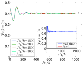
Figure 2: (Color online) Evolution of the population on the $k=0$ quasi-momentum state $\langle\hat{F}_{2}(k=0)\rangle$ after the second expansion. The parameters are $(N,M_{0},M_{1},M_{2})=(50,100,200,300)$. The dotted line indicates the result with the “initial” state being the (first) generalized Gibbs ensemble (GGE) density matrix $\Xi_{gge1}$. Other lines correspond to results with the “initial” states being $\psi(t_{1})$, with the value of $t_{1}$ varied. The markers on the right ends of the lines indicate the predicted values of the second GGEs. The insert shows the time evolution of the population on the $k=0$ quasi-momentum state $\langle\hat{F}_{1}(k=0)\rangle$ after the first expansion.

In the intervals of $t\leq 0$, $0<t<t_{1}$, and $t\geq t_{1}$, the volume (number of sites) of the system is $M_{0}$, $M_{1}$, and $M_{2}$, and thus the corresponding Hamiltonians will be denoted as $H_{0}$, $H_{1}$, and $H_{2}$, respectively. They are of the form $H_{i}=-J\sum_{j=L_{i}}^{R_{i}-1}(b_{j}^{\dagger}b_{j+1}+b_{j+1}^{\dagger}b_{j})$, $0\leq i\leq 2$. Here $J$ is the hopping strength, and $L_{i}=(M_{2}-M_{i})/2+1$ and $R_{i}=(M_{2}+M_{i})/2$ denote the left- and right-most sites accessible to the bosons, respectively. The creation and annihilation operators satisfy the usual bosonic commutation relations plus the hard-core constraint $b_{j}^{2}=b_{j}^{\dagger 2}=0$, so that each site can be occupied by at most one boson. By using the Jordan-Wigner transformation $(b_{j}^{\dagger},b_{j})=(c_{j}^{\dagger},c_{j})\prod_{j^{\prime}=1}^{j-1}e^{-i\pi c_{j^{\prime}}^{\dagger}c_{j^{\prime}}}$, where $c_{j}$ ($c_{j}^{\dagger}$) is the fermionic annihilation (creation) operator, $H_{i}$ is mapped to a free fermion one, $H_{i}=-J\sum_{j=L_{i}}^{R_{i}-1}(c_{j}^{\dagger}c_{j+1}+c_{j+1}^{\dagger}c_{j})$. This Hamiltonian can be readily diagonalized as $H_{i}=\sum_{q=1}^{M_{i}}\varepsilon_{q}^{(i)}\eta^{(i)\dagger}_{q}\eta_{q}^{(i)}$, with $\varepsilon_{q}^{(i)}=-2J\cos\left(\pi q/(M_{i}+1)\right)$ and $\eta_{q}^{(i)}=\sqrt{\frac{2}{M_{i}+1}}\sum_{j=L_{i}}^{R_{i}}c_{j}\sin(q\pi(j-L_{i}+1)/(M_{i}+1))$. The initial state is then simply a Fermi-sea state $\psi_{0}=\prod_{q=1}^{N}\eta^{(0)\dagger}_{q}|0\rangle$.

From $H_{0}$ to $H_{1}$, the wave function evolves as $\psi(t_{1})=e^{-iH_{1}t_{1}/\hbar}\psi_{0}$, and the (first) GGE density matrix is defined as $\Xi_{gge1}=\frac{1}{\Theta_{1}}\exp[-\sum_{q=1}^{M_{1}}\lambda_{q}^{(1)}c_{q}^{(1)\dagger}c_{q}^{(1)}]$. Here the parameter $\lambda_{q}^{(1)}$ is determined by the initial state, $tr(c_{q}^{(1)\dagger}c_{q}^{(1)}\Xi_{gge1})=\langle\psi_{0}|c_{q}^{(1)\dagger}c_{q}^{(1)}|\psi_{0}\rangle$, and $\Theta_{1}$ is a normalization factor (or partition function). It is found in rigol07 , argued in cazalilla11 , and verified in Fig. 2 below that for $t_{1}$ large enough, the momentum distribution (or populations on the quasi-momentum states, here $k=-M_{1}/2,-M_{1}/2+1,\cdots,M_{1}/2-1$)

$$\hat{F}_{1}(k)=\frac{1}{M_{1}}\sum_{j,j^{\prime}=L_{1}}^{R_{1}}e^{-i2\pi k(j-j^{\prime})/M_{1}}b_{j^{\prime}}^{\dagger}b_{j}$$ (9)

with respect to $\psi(t_{1})$ can be accurately reproduced by using $\Xi_{gge1}$, i.e., $\langle\psi(t_{1})|\hat{F}_{1}(k)|\psi(t_{1})\rangle\simeq tr(\hat{F}_{1}(k)\Xi_{gge1})$.

Now from $H_{1}$ to $H_{2}$, the $H_{2}$-evolved wave function at $t=t_{1}+t_{2}$ is given by $\psi(t_{1}+t_{2})=e^{-iH_{2}t_{2}/\hbar}\psi(t_{1})$. For our purpose, we replace the “initial” state $\psi(t_{1})$ by $\Xi_{gge1}$ and define the $H_{2}$-evolved GGE density matrix $\Xi_{gge1}(t_{2})=e^{-iH_{2}t_{2}/\hbar}\Xi_{gge1}e^{iH_{2}t_{2}/\hbar}$. We then study the momentum distribution ($k=-M_{2}/2,-M_{2}/2+1,\cdots,M_{2}/2-1$)

$$\hat{F}_{2}(k)=\frac{1}{M_{2}}\sum_{j,j^{\prime}=L_{2}}^{R_{2}}e^{-i2\pi k(j-j^{\prime})/M_{2}}b_{j^{\prime}}^{\dagger}b_{j}$$ (10)

with respect to $\psi(t_{1}+t_{2})$ and $\Xi_{gge1}(t_{2})$. The results are shown in Fig. 2.

In the insert of Fig. 2, we see that after the first expansion, the population on the $k=0$ quasi-momentum state $\langle\psi(t_{1})|\hat{F}_{1}(k=0)|\psi(t_{1})\rangle$ relaxes to the steady value predicted by the GGE density matrix $\Xi_{gge1}$ eventually. This proves the predictive power of the GGE after the first expansion. What Fig. 2 highlights is that, if the time of the second expansion $t_{1}$ is chosen to belong to the steady regime, the later evolution of the population on the $k=0$ quasi-momentum state $\langle\psi(t_{1}+t_{2})|\hat{F}_{2}(k=0)|\psi(t_{1}+t_{2})\rangle$ can be accurately reproduced by $tr(\hat{F}_{2}(k=0)\Xi_{gge1}(t_{2}))$. Their lines coincide with each other not only in the asymptotic limit but even on details during the transitory period. Note that since the latter is independent of $t_{1}$, this necessarily implies that the former is insensitive to the value of $t_{1}$, as is indeed the case. Overall, Fig. 2 is a remarkable demonstration of the fact that the GGE density matrix $\Xi_{gge1}$ shares with the relaxed state $\psi(t_{1})$ not only the value of the momentum distribution, but also the response to a second quench. Or in the perspective of the state $\psi(t_{1})$, it has relaxed to be virtually indistinguishable from the GGE state $\Xi_{gge1}$, neither by static nor dynamical criterions.

In Fig. 2, we have also studied whether the steady value of $\hat{F}_{2}(k=0)$ after the second quench can be described by a second GGE density matrix $\Xi_{gge2}$, which is defined as $\Xi_{gge2}=\frac{1}{\Theta_{2}}\exp[-\sum_{q=1}^{M_{2}}\lambda_{q}^{(2)}c_{q}^{(2)\dagger}c_{q}^{(2)}]$, with the parameter $\lambda_{q}^{(2)}$ determined by the condition $tr(c_{q}^{(2)\dagger}c_{q}^{(2)}\Xi_{gge2})=tr(c_{q}^{(2)\dagger}c_{q}^{(2)}\Xi_{gge1})$ or $tr(c_{q}^{(2)\dagger}c_{q}^{(2)}\Xi_{gge2})=\langle\psi(t_{1})|c_{q}^{(2)\dagger}c_{q}^{(2)}|\psi(t_{1})\rangle$ depending on whether the “initial” state is $\Xi_{gge1}$ or $\psi(t_{1})$. The result is that the second GGEs do predict the steady values correctly; moreover, they agree with each other very well. This is one more evidence that the relaxed wave function $\psi(t_{1})$ is virtually indistinguishable from the GGE $\Xi_{gge1}$.

In summary, we have investigated and verified the relevance of the GGEs in the dynamical response of the two integrable models of transverse Ising model and one-dimensional hard-core bosons. Once having relaxed to have its properties correctly predicted by the GGE, the system behaves as if it were indeed in the GGE state—its response to the second quench can be accurately reproduced by the GGE even to details. On one hand, this result is a welcome complement to previously established result that the GGEs are relevant in predicting the static properties of the systems after the first quench. The two now combine to present a more complete story of the GGE and beckon more confidence on it. On the other hand, this result also gives us a sense of “dynamical typicality” gemmer , which is also observed in the (non-integrable) Bose-Hubbard model previously zjm . Finally, though here we have been dealing with integrable systems only, a lesson may also be drawn for non-integrable systems. A closed non-integrable system might well be a pure state yet virtually indistinguishable neither by static nor by dynamic criterions from a canonical ensemble.

We acknowledge Institute of Physics, CAS for funding.

References

(1)
A. Polkovnikov, K. Sengupta, A. Silva, and M. Vengalattore,
Rev. Mod. Phys. 83, 863 (2011).
(2)
Though the notion of quantum integrability is still a
subject of debate, see J.-S. Caux and J. Mossel, J. Stat.
Mech. P02023 (2011).
(3)
T. Kinoshita, T. Wenger, and D. S. Weiss, Nature (London)
440, 900 (2006).
(4)
M. Rigol, V. Dunjko, V. Yurovsky, and M. Olshanii, Phys.
Rev. Lett. 98, 050405 (2007); M. Rigol, A.
Muramatsu, and M. Olshanii, Phys. Rev. A 74,
053616 (2006).
(5)
E. T. Jaynes, Phys. Rev. 106, 620 (1957);
108, 171 (1957).
(6)
M. A. Cazalilla, Phys. Rev. Lett. 97, 156403
(2006).
(7)
P. Calabrese and J. Cardy, J. Stat. Mech. P06008 (2007).
(8)
M. Eckstein and M. Kollar, Phys. Rev. Lett. 100,
120404 (2008).
(9)
D. Fioretto and G. Mussardo, New J. Phys. 12,
055015 (2010).
(10)
P. Calabrese, F. H. L. Essler, and M. Fagotti, Phys. Rev.
Lett. 106, 227203 (2011).
(11)
T. Caneva, E. Canovi, D. Rossini, G. E Santoro, A. Silva,
J. Stat. Mech. P07015 (2011).
(12)
M. A. Cazalilla, A. Iucci, and M.-C. Chung,
arXiv:1106.5206.
(13)
Of course, the GGE does have its limitations, e.g., it can
not capture the possible correlations present in a generic
initial state and thus may fail to predict the asymptotic
values of physical relevant observables or correlations
between the eigenmodes. See Polkovnikov , D. M.
Gangardt and M. Pustilnik, Phys. Rev. A 77,
041604(R) (2008); J. Lancaster and A. Mitra, Phys. Rev. E
81, 061134 (2010).
(14)
J. M. Zhang, C. Shen, and W. M. Liu, Phys. Rev. A
83, 063622 (2011).
(15)
E. Lieb, T. Shultz, and D. Mattis, Ann. Phys. (N.Y.)
16, 407 (1961); P. Pfeuty, Ann. Phys. 57,
79 (1970).
(16)
See the supplementary material.
(17)
Here and below the sign does not mean the
limit but just the typical value. Actually, for a finite
, the basic correlators are almost periodic
functions of and they have no limits at all. However,
for large enough, the probability of recurrence is
practically irrelevant.
(18)
K. Sengupta, S. Powell, and S. Sachdev, Phys. Rev. A
69, 053616 (2004).
(19)
C. Bartsch and J. Gemmer, Phys. Rev. Lett. 102,
110403 (2009).