Mapping the Shores of the Brown Dwarf Desert III: Young Moving Groups

Abstract

We present the results of an aperture masking interferometry survey for substellar companions around 67 members of the young ($\sim$ 8–200 Myr) nearby ($\sim$ 5–86 pc) AB Doradus, $\beta$ Pictoris, Hercules-Lyra, TW Hya, and Tucana-Horologium stellar associations. Observations were made at near infrared wavelengths between 1.2–3.8 $\mu$m using the adaptive optics facilities of the Keck II, VLT UT4, and Palomar Hale Telescopes. Typical contrast ratios of $\sim$ 100–200 were achieved at angular separations between $\sim$ 40–320 mas, with our survey being 100% complete for companions with masses below $\sim$0.25 $M_{\odot}$ across this range. We report the discovery of a $0.52\pm 0.09$ $M_{\odot}$ companion to HIP 14807, as well as the detections and orbits of previously known stellar companions to HD 16760, HD 113449, and HD 160934. We show that the companion to HD 16760 is in a face-on orbit, resulting in an upward revision of its mass from $M_{2}\sin i\sim 14$ $M_{\rm J}$ to $M_{2}=0.28\pm 0.04$ $M_{\odot}$. No substellar companions were detected around any of our sample members, despite our ability to detect companions with masses below 80 $M_{\rm J}$ for 50 of our targets: of these, our sensitivity extended down to 40 $M_{\rm J}$ around 30 targets, with a subset of 22 subject to the still more stringent limit of 20 $M_{\rm J}$. A statistical analysis of our non-detection of substellar companions allows us to place constraints on their frequency around $\sim$ 0.2–1.5 $M_{\odot}$ stars. In particular, considering companion mass distributions that have been proposed in the literature, we obtain an upper limit estimate of $\sim$ 9–11% for the frequency of 20–80 $M_{\rm J}$ companions between 3–30 AU at 95% confidence, assuming that their semimajor axes are distributed according to $d\mathcal{N}/da\propto a^{-1}$ in this range.

1. Introduction

In the past few years, direct imaging surveys have begun to build up a picture of the mass and semimajor axis distributions of substellar companions at separations beyond $\sim$ 20–30 AU (eg. Biller et al., 2007; Carson et al., 2006; Chauvin et al., 2010; Kasper et al., 2007; Lafrenière et al., 2007; Lowrance et al., 2005; Masciadri et al., 2005; Metchev & Hillenbrand, 2009). Meanwhile, statistical analyses of radial velocity results have tended to focus on objects with masses below $\sim$ 10$M_{\rm J}$ out to separations of $\sim$ 3 AU (Cumming et al., 2008; Howard et al., 2010). However, given the observational biases of radial velocity and direct imaging surveys, the separation range of $\sim$ 3–30 AU has remained relatively unexplored.

Aperture masking interferometry is a direct detection technique that is well suited for detecting substellar companions with masses of $\sim$ 10 $M_{\rm J}$ and semimajor axes within $\sim$ 30 AU around young, nearby stars. For instance, it has been used to conduct surveys for substellar companions around members of the Upper Scorpius (Kraus et al., 2008) and Taurus-Auriga (Kraus et al., 2011) associations, as well as to measure the dynamical mass of the brown dwarf companion to GJ 802b (Ireland et al., 2008), show that CoKu Tau/4 is a binary system rather than a transitional disk (Ireland & Kraus, 2008), and place limits on possible companions existing within 10 AU of HR 8799 (Hinkley et al., 2011). Recently, the technique has also produced the first direct detection of a young exoplanet still undergoing formation within the transitional disk of LkCa15 (Kraus & Ireland, submitted) and a similar detection of an object within the gap of the T Cha disk (Huélamo et al., 2011).

This paper presents the results of an aperture masking survey of 67 members of the AB Doradus (AB Dor), $\beta$ Pictoris ($\beta$ Pic), Hercules-Lyra (Her-Lyr), Tucana-Horologium (Tuc-Hor), and TW Hya (TWA) moving groups. At least 49 of our targets have been observed previously as part of deep imaging surveys, but these observations have typically been sensitive to different orbital separations than those that are probed here. We chose our targets based on their youth (8–200 Myr) and proximity (5–86 pc). The former ensures that any substellar companions are still glowing relatively brightly at infrared wavelengths following their recent formation, while the latter allows smaller absolute separations to be explored for a given angular separation.

The paper is organized as follows. In Section 2, we provide a brief overview of the aperture masking technique. In Section 3, we describe our survey sample. In Section 4 we summarize the observations that were made and how the data were reduced. In Section 5, we explain how we searched for companions to the target stars in the reduced data and how we derived the survey detection limits. In Section 6 we report our results, including the detections and orbits for stellar companions around HIP 14807, HD 16760, HD 113449, and HD 160934. However, no substellar companions were detected, and in Section 7 we present a statistical analysis of this null result before concluding in Section 8.

2. Aperture Masking

The aperture masking technique works by placing an opaque, perforated mask at or near the pupil plane of a telescope (Fizeau 1868; Michelson 1891a; more recently, see Tuthill et al. 2000, 2006, 2010). This converts the single aperture into a multi-element interferometer. Each pair of holes in the mask acts as an interferometric baseline, resulting in an interferogram being projected onto the image plane.

The complex visibility $V$ (Michelson, 1891b) of the source brightness distribution $S$ is sampled by taking the 2D Fourier transform of the measured interferogram $I$. This follows from the Van Cittert-Zernike Theorem, which states that the normalized complex visibility is equal to the Fourier transform of the brightness distribution:

$$V = \frac{\tilde{S}}{S_{0}}$$ (1)

where the tilde denotes the Fourier transform and $S_{0}$ is the total source flux. Since the detected image is the convolution of the instrumental point spread function (PSF) and the source brightness distribution, this leads to:

$$V = \frac{\tilde{I}}{S_{0}\,\tilde{P}}$$ (2)

where $\tilde{P}$ denotes the Fourier transform of the PSF. In practice, the PSF is measured by observing an unresolved calibrator star, i.e. a point source, which has unit complex visibility $V=1$.

In this study, we used non-redundant aperture masks, with each baseline pair corresponding to a unique point on the spatial frequency plane. We used masks with 7, 9, and 18 holes, giving 21, 36, and 153 independent baselines, respectively. Hole diameters and transmission fractions are provided in Table 1. The subaperture configurations on the masks were designed to provide a uniform and isotropic sampling of the complex visibility function, with the specific mask chosen to observe a given target depending on the target’s brightness and the expected sources of systematic error. For example, although the 18 hole masks had slightly longer baselines than the 7 or 9 hole masks, they had lower total throughput with a broader PSF. This meant that they could only be used with narrow band filters, which restricted their use to brighter targets.

To identify faint companions around our targets, we used a quantity derived from the complex visibility known as the closure phase $\Theta$ (Jennison, 1958; Baldwin et al., 1986). The closure phase is obtained by adding the complex visibility phases around a closure triangle of subapertures. Explicitly, if we denote the measured complex visibility phase between the $i$th and $j$th subapertures as $\varphi_{ij}$, the intrinsic complex visibility phase as $\phi_{ij}$, and a phase error due to atmospheric and instrumental effects across the $i$th aperture as $\eta_{i}$, then we have:

$$\varphi_{ij} = \phi_{ij}+\eta_{i}-\eta_{j}$$

$$\varphi_{ij} = \phi_{jk}+\eta_{j}-\eta_{k}$$

$$\varphi_{ij} = \phi_{ki}+\eta_{k}-\eta_{i}$$ (3)

Importantly, the diameter of the mask holes are chosen to ensure that the wavefront phase variations across each subaperture are approximately constant so that they can be neglected. Combining aperture masking with adaptive optics allows subaperture diameters that are larger than the atmospheric Fried parameter and exposure times that are longer than the atmospheric coherence time to be used, providing a greater through-put of photons. It follows that the $\eta_{i}$ terms cancel out when we take the closure phase sum:

$$\Theta_{ijk} = \phi_{ij}+\phi_{jk}+\phi_{ki}$$ (4)

where $\Theta_{ijk}$ is the closure phase of the triangle $ijk$.

The independence of the closure phase quantity from major sources of systematic error allows us to achieve the full interferometric resolution according to the Michelson criterion, which is equal to $\lambda/2B$, where $\lambda$ is the observing wavelength and $B$ is the longest baseline on our mask. This is the smallest angular separation for which two point sources would be fully resolved. Given that the longest baseline of the masks used in this study span nearly the entire telescope aperture, this corresponds to angular scales of roughly half the single-aperture diffraction limit.

3. Survey Sample

Figure 1.— The 67 survey targets binned according to the spectral types (top panel) and masses (bottom panel) listed in Table 3.

In 2007, our group initiated a search for close, faint companions around young, nearby stars using the aperture masking facilities installed on the 5.1 m Hale telescope at Palomar Observatory in California. In subsequent years (2007–2011) the survey was extended and made use of similar facilities installed on the 10 m Keck II telescope at Keck Observatory in Hawaii and the 8.2 m VLT UT4 telescope at the VLT Observatory in Chile.

Our final survey sample consisted of 67 proposed members of the AB Dor (Zuckerman et al., 2004), $\beta$ Pic (Zuckerman et al., 2001a), Her-Lyr (Fuhrmann, 2004), Tuc-Hor (Zuckerman et al., 2001b), and TWA (Kastner et al., 1997) moving groups. A concise summary of the sample is provided in Table 2 while the full list is given in Table 3. Figure 1 shows the sample members binned according to spectral type and masses.

In selecting our targets, we noted that many of the moving group members have already been identified as binary systems. The presence of a binary companion within $\sim$ 1″ of a target star reduces the ability of aperture masking to detect additional companions, because the interferograms will overlap. Also, similar brightness companions at separations of $\sim$1.5–3″ can prevent the adaptive optics system from achieving a stable lock on the target. For these reasons, we chose not to include any targets in our sample that were known to be affected by such issues.

We also emphasize the difficulty of assigning moving group membership to individual stars. Consequently, it is possible that not all objects in our sample are necessarily young. In particular, the moving group memberships of nine of our targets (HD 89744, HD 92945, GJ 466, EK Dra, HIP 30030, TWA-21, TWA-6, TWA-14, TWA-23) were either unable to be confirmed or else ruled to be unlikely by Torres et al. (2008) using a dynamical convergence analysis. Furthermore, the existence of Her-Lyr as a genuine moving group is not yet as well-established as the others. To investigate how sensitive our statistical analysis presented in Section 7.2 is to the uncertain membership of these targets, we repeated the calculations separately with them included and then removed from the sample.

4. Observations and Data Reduction

We observed our program objects over the course of twelve observing runs using the facility adaptive optics imagers at Palomar (PHARO), Keck (NIRC2), and VLT (CONICA) between April 2007 and April 2011. Each camera has aperture masks installed at (Palomar, VLT) or near (Keck) the pupil stop wheels. The central wavelengths and bandpass widths for each filter used are listed in Table 4 and details of our observations are summarized in Table 5. Observing conditions varied widely, but we attempted to match the observations to the appropriate conditions. Most of our brighter targets were observed through clouds or marginal seeing as they were the only ones we could lock the AO system on, while our fainter targets were typically observed under better conditions.

Our observing strategy has been described previously in Kraus et al. (2008). Each observation consisted of 1–3 target-calibrator pairs, usually with $\sim$ 10–20 frames per block. We tried to choose calibrators with optical and near-infrared brightnesses that were similar to those of the target, rather than calibrators that were necessarily brighter. This was done due to concerns about the magnitude-dependence of non-common path errors in the adaptive optics system. For targets of brightness $R\lesssim 7$, calibrators were chosen from the stable radial velocity stars of Nidever et al. (2002). For fainter stars, we could not explicitly choose calibrators that had been vetted for close binaries, so we simply chose nearby 2MASS sources with similar colors and brightnesses. In all cases, we tried to select calibrators that appeared to be single and unblended in the 2MASS images, as well as close to the target on the sky ($\lesssim$ 10 deg for the Nidever et al sources and $\lesssim$ 3 deg for the 2MASS sources). In addition to reducing overhead times, using nearby calibrators helped to minimize residual wavefront errors introduced by long telescope slews.

Data reduction was performed using our group’s custom-written IDL pipeline (for further details, see Lloyd et al. 2006, Ireland et al. 2008, and Kraus et al. 2008). Complex visibilities were extracted by Fourier-inverting the cleaned data cubes and sampling the $uv$-plane at points corresponding to the mask baselines. Calibration was performed by subtracting the calibrator complex visibility phases from the complex visibility phases of the science targets.

5. Binary Model Fitting

We used the same method as Kraus et al. (2008, 2011) to search for companions to our targets over the separation range 20–320 mas. We only used closure phases in our binary model fitting, discarding the visibility amplitudes as these are more affected by systematic errors. The parameters we fit for were the angular separation $\rho$ between the primary and companion, the position angle $\theta$ of the companion, and the brightness contrast ratio $C=f_{p}/f_{c}$, where $f_{p}$ and $f_{c}$ were the fluxes of the primary and companion, respectively. Fitting was performed by initially fixing a high contrast ratio of $C=250$ and generating the corresponding model closure phases for each point on a grid of angular separations spanning $20<\rho<320$ mas and position angles spanning $0<\theta<360$ deg. The point on the $\rho$–$\theta$ grid giving the lowest $\chi^{2}$ for the measured closure phase values was then taken to be the starting point for a steepest-descent search in which all three model parameters ($C$, $\rho$, $\theta$) were allowed to vary. The initial grid search ensured that the final minimum reached corresponded to the global minimum.

The binary fit was considered to be bona fide if it passed a 99.5% detection criterion, which has been explained in Kraus et al. (2008, 2011). This was done by generating 10 000 artificial closure phase data sets with Fourier plane sampling that was identical to that of the measured data. Each artificial closure phase was randomly sampled from a Gaussian distribution with a mean of zero, corresponding to an unresolved point source, and the same variance as the corresponding measured value. A best-fit companion contrast $C$ was then obtained for each set of artificial closure phases using $\chi^{2}$ minimization at each point on the $\rho$–$\theta$ grid. Once again, by searching over the entire grid we ensured that the global minimum was identified. A 99.9% detection threshold was then defined separately for five contiguous annuli (20–40 mas, 40–80 mas, 80–160 mas, 160–240 mas, 240–320 mas), corresponding to the 0.1th percentile of the best-fit contrasts obtained for the artificial data sets within that annulus. In other words, if the target was a point source instead of a binary, there was only a 0.1% chance that the measured closure phases would give a best-fit contrast lower than the threshold value in the annulus corresponding to the best-fit separation. This corresponds to a $5\times 0.1\%=0.5\%$ false alarm probability across the full 20–320 mas range. Therefore, if the best-fit model satisfied this condition, the detection was considered to be real at 99.5% confidence.

It was important to ensure that any high probability ($>$99.5%) detections were not caused by companions around one of the calibrators rather than around the science target. A small number of such false alarms ($\sim$ 5) did occur during the course of our analysis. Such cases were usually quite straightforward to identify by systematically repeating the calibration and binary fitting, excluding one calibrator at a time. Given that the calibrators did not have known ages, but were likely to be $\sim$ Gyr old, any companions detected around them were almost certainly not substellar, and so they were not considered further.

6. Results

Using the method described in Section 5, we identified stellar companions to four of our AB Dor targets (HIP 14807, HD 16760, HD 113449, HD 160934) and report our best-fit binary solutions in Table 6. Of these, the companion to HIP 14807 is a new discovery while the companions to HD 16760, HD 113449, and HD 160934 are the same as those discovered independently using radial velocity (Bouchy et al., 2009; Sato et al., 2009; Cusano et al., 2009, 2010; Gálvez et al., 2006). We describe the detected companions in Sections 6.1–6.4, and present our full survey detection limits in Section 6.5.

6.1. HIP 14807

A companion was clearly detected in our Keck observations of HIP 14807 on 2009 November 21 (MJD 55156.2) at an angular separation of $\rho=28.74\pm 0.19$ mas with a contrast ratio of $C=3.00\pm 0.06$ in the CO filter. Assuming a system age of $110\pm 40$ Myr, interpolation of the NextGen isochrones of Baraffe et al. (1998) gives an estimated companion mass of $0.52\pm 0.09$ $M_{\odot}$, which includes the uncertainty in the age and distance, as well as the uncertainty in the fitted contrast.

The companion was also detected at high confidence in the Palomar data from 2007 November 29 (MJD 54433.1), with a fitted contrast ratio of $C=10.15\pm 3.71$. However, this error bar is neither symmetric nor realistic, as there is a strong degeneracy between contrast and separation for small separations in aperture masking data sets. This is illustrated in Figure 2 (see also Figure 7 in Pravdo et al. 2006, Table 2 in Ireland et al. 2008, and Figure 2 in Huélamo et al. 2011). A fuller discussion of this degeneracy is provided in Section 2.1 of Martinache et al. (2009). In cases such as these, quick data sets were taken with only one or two calibration observations. As a result, the quoted error bars are not necessarily accurate at the few tens of a percent level, because the dispersion between calibrators is used to estimate the errors in the closure phases. Despite this, global orbital fitting to multiple aperture masking data sets has been performed successfully by using a single contrast for all epochs, with the resulting astrometric fits being consistent with those obtained using other techniques, and having reduced $\chi^{2}$ of order unity (eg. Dupuy et al. 2009b).

Figure 2.— The contrast/separation degeneracy for the fit to the HIP 14807 data taken in K band on 2007 Nov 29 (MJD 54433.1), showing the default fit from our pipeline (triangle) and the fit after fixing the contrast (star). The third axis of position angle has been integrated over to give a two-dimensional likelihood plot. Contours are nominally at 90, 99, 99.9, and 99.99% confidence.

For these reasons, we redid the binary fitting to the MJD 54433.1 data using a prior on the contrast determined from the other well-constrained fit to the MJD 55156.2 data. The results of this revised fit are given in Table 7.

6.2. HD 16760

HD 16760 is unusual because it shows signs of being both young and old. Its youth is implied by its high lithium abundance, as well as its physical association with the active star HIP 12635 and a common proper motion with the AB Dor group (Zuckerman et al., 2004; Torres et al., 2008). Its old age is implied by its low $v\sin i$ value ($2.8\pm 1.0$  km s^-1, Bouchy et al. 2009; $0.5\pm 0.5$  km s^-1, Sato et al. 2009) and its low Ca H & K activity index ($\log R^{\prime}_{HK}=-4.93$, Sato et al. 2009; $\log R^{\prime}_{HK}=-5.0\pm 0.1$, Bouchy et al. 2009), which is consistent with field dwarfs ($\log R^{\prime}_{HK}=-4.99\pm 0.07$, Mamajek & Hillenbrand 2008) and inconsistent with high probability members of the 625 Myr Hyades cluster ($\log R^{\prime}_{HK}=-4.47\pm 0.09$, Mamajek & Hillenbrand 2008) and other young stars (see Tables 5–8 of Mamajek & Hillenbrand 2008). However, we note that this system is not the only example of a binary pair showing contradictory age indicators: when examining the activity consistency of known binary pairs, Mamajek & Hillenbrand (2008) identified a similar case of an inactive primary with an active companion (HD 137763 A/B).

Previous radial velocity measurements have shown that HD 16760 possesses a close companion (Sato et al., 2009; Bouchy et al., 2009), for which Sato and coworkers derived a minimum mass $M_{2}\,\sin i$ value of $13.13\pm 0.56$ $M_{\rm J}$, while Bouchy and coworkers obtained a similar value of $14.3\pm 0.9$ $M_{\rm J}$. We clearly detected this companion in our Keck data from 2008 December 23 (MJD 54823.2), 2009 August 6 (MJD 55049.6) and 2009 November 20 (MJD 55155.3) (Table 6). Taking the weighted mean of the well-constrained isochrone mass estimates, we obtain a mass of $M_{2}=0.28\pm 0.04$ $M_{\odot}$ for the companion, which includes the uncertainty in the age, distance and fitted contrasts. This places it well within the stellar mass range.

Meanwhile, due to degeneracy between contrast and separation (see Section 6.1), combined with mediocre data quality, the separation derived from the MJD 55155.3 K band data was inconsistent with the separation derived from the J and H band data taken on the same night. For this reason, we obtained a further observation the following night with the CO filter, which has a very similar bandpass to the Kcont filter (see Table 4; we had intended to use the Kcont filter, but there was a mix-up in the filter selections). The binary parameters derived from this follow-up observation are in close agreement with the values obtained from the J and H band observations.

We also repeated the fit to the degenerate K band data with a prior on the contrast obtained by combining the fitted contrasts to the other K band epochs. The system properties derived from this re-analysis are reported in Table 7, and agree with the values obtained for the J and H band data sets. We note, however, that the calibration error added in quadrature to obtain a reduced $\chi^{2}$ of unity for this fit was 1.8 degrees. This is unusually large and suggests that the quoted errors for the inferred parameters are likely to be underestimated somewhat.

Using our multi-epoch data, we were able to derive an orbital solution for the companion. To do this, we fixed the values for the time of periastron $T_{0}$, orbital period $P$, orbital eccentricity $e$, and argument of periastron $\omega$ published for the radial velocity orbit from Sato et al. (2009). We were not able to fit for the orbital inclination $i$ using our aperture masking astrometry data because we only measure the axis ratio of the visual orbit, and this varies with the cosine of the inclination. Hence, we are not sensitive to small changes in $i$ when $i$ is near zero, as is the case here. Instead, we combined the model-dependent mass estimate obtained from the aperture masking results with the value for $M_{2}\,\sin i$ derived from the radial velocity results to calculate $i=2.6\pm 0.5$ deg. Then with these parameters held fixed, we inferred values for the longitude of the ascending node $\Omega$ and semimajor axis $a$ by fitting to the aperture masking astrometry listed in Tables 6 and 7. The final orbital solution is reported in Table 8, and plotted in Figure 3.

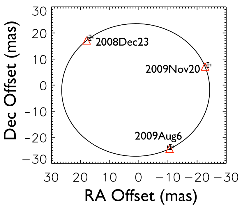
Figure 3.— Plotted orbital solution for the companion to HD 16760. The black crosses show the aperture masking astrometry points with associated uncertainties and the red triangles mark the corresponding epochs of the orbital solution.

Lastly, we note that the rotational velocity of the primary is revised upwards from $v\sin i\sim 0.5$–$4$  km s^-1 to $v\sim$20–25  km s^-1, a value that is more in line with other members of AB Dor. However, the low Ca H & K emission of HD 16760 remains unexplained. The only reason we might expect to see an inclination dependence in the strength of $\log R^{\prime}_{HK}$ is if the Ca H & K emission varies with latitude on a star, such that polar areas show little emission compared to equatorial regions. We are not aware of any model that would predict this effect.

6.3. HD 113449

We detected a companion around HD 113449 in six of our data sets taken at Palomar and Keck between 2007 Apr 6 and 2010 Apr 25 (Table 6). Four of these data sets (MJD 54196.3, MJD 54634.2, MJD 54821.7, MJD 553311.4) were well-constrained, and taken together imply a companion mass of $0.51\pm 0.01$ $M_{\odot}$ based on the NextGen isochrones of Baraffe et al. (1998), including the uncertainty in the age, distance and fitted contrasts. The other two data sets, however, gave fits that were degenerate in contrast and separation, as has been described above. For the first of these (MJD 54197.6), we repeated the analysis with a prior on the separation taken from the well-constrained fit to the previous night’s data (see footnote in Table 6). For the second case (MJD 54252.1), the analysis was repeated with a prior on the contrast taken from the well-constrained solutions obtained for the four other H band data sets (see Table 7).

The companion we report here was first announced by Cusano et al. (2009, 2010) subsequent to the commencement of our survey. Using radial velocity measurements, those authors obtained a value of $F(M_{1},M_{2},i)=0.0467\pm 0.0006$ $M_{\odot}$ for the spectroscopic mass function and estimated a secondary-to-primary mass ratio of $q=0.57\pm 0.05$. In addition, using astrometry measurements made with the VLT-I they obtained a value of $i=57\pm 3^{\circ}$ for the inclination, $\Omega=124\pm 4^{\circ}$ for the longitude of the ascending node and $a=0.750\pm 0.030$ AU for the semimajor axis.

We computed an orbital solution for the companion using our aperture masking astrometry (Tables 6 and 7), allowing $i$, $a$, and $\Omega$ to vary as free parameters in our fitting, while holding $P$, $T_{0}$, $e$ and $\omega$ fixed at the values determined Cusano and coworkers. However, we found that we could not obtain a reasonable $\chi^{2}$ value with the period of $P=215.9$ days reported by those authors. Instead, an acceptable fit was made when we allowed the period to be a free parameter, obtaining $P=216.9$ days. The best-fit parameters are reported in Table 8 and the corresponding orbit is plotted in Figure 5. In particular, our fitted value of $\Omega=202.0\pm 1.6^{\circ}$ does not agree with the value of $\Omega=124\pm 4^{\circ}$ reported in Cusano et al. (2010), but as the details of those VLT-I observations are not given, we cannot make a further comparison. Lastly, the dynamical mass of the system ($M_{\rm{tot}}=1.10\pm 0.09$ $M_{\odot}$) appears to be underestimated by $\sim 2\sigma$ when compared to the isochrone-determined masses ($M_{1}=0.84\pm 0.08$ $M_{\odot}$ and $M_{2}=0.51\pm 0.01$ $M_{\odot}$). As the orbital period is $\sim$1 year and the astrometric semimajor axis is comparable to the parallax, examining this discrepancy in more detail would require refitting to the raw HIPPARCOS data.

6.4. HD 160934

We detected a companion around HD 160934 in our Palomar data taken on 2008 June 23 (MJD 54640.3) and Keck data taken on 2010 April 26 (MJD 55312.6) and 2011 April 23 (MJD 55674.6). The binary solutions are all in excellent agreement (Table 6). We obtain a value of $0.54\pm 0.01$ $M_{\odot}$ for the companion mass by combining the estimates from each epoch.

This companion was first reported by Gálvez et al. (2006), who identified HD 160934 as a spectroscopic binary with an estimated period of $\sim$ 17.1 years and an eccentricity of $e$ $\sim$ 0.8. However, these were preliminary values based on limited phase sampling, and a period of approximately half this is also consistent with the data. In fact, this shorter period is the one preferred by Griffin & Filiz Ak (2010), who repeated the fit to the same data with a small number of more modern radial velocity measurements.

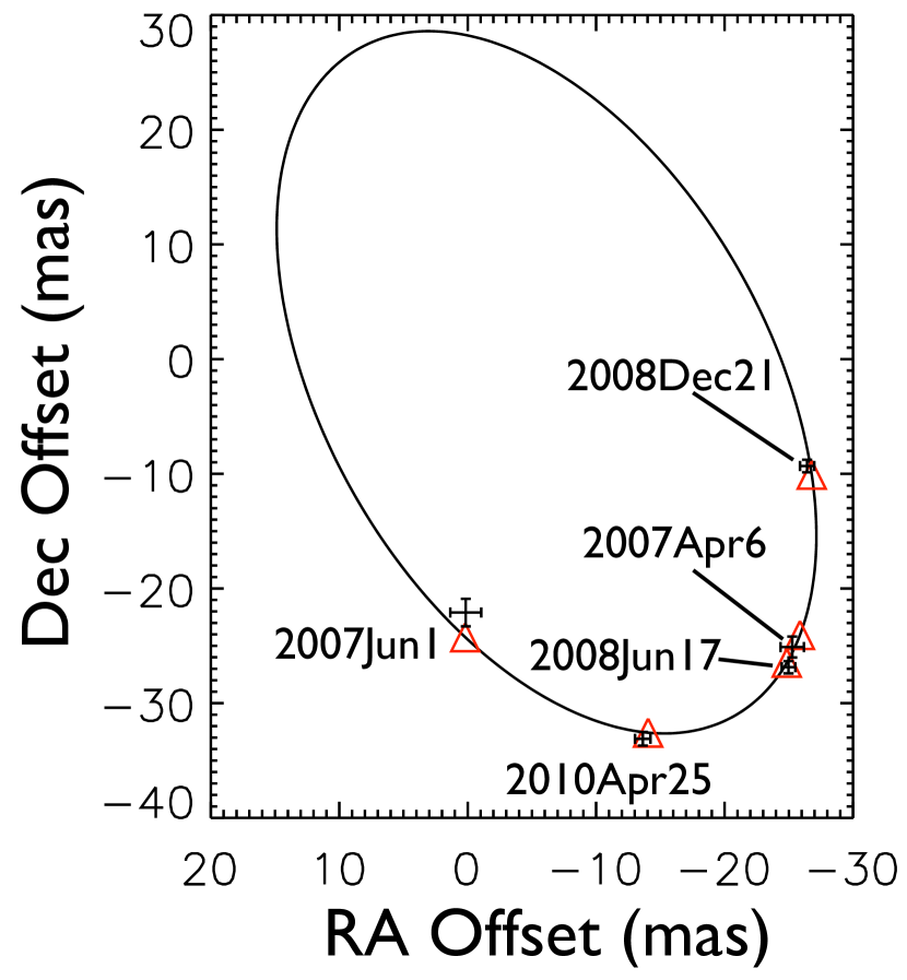
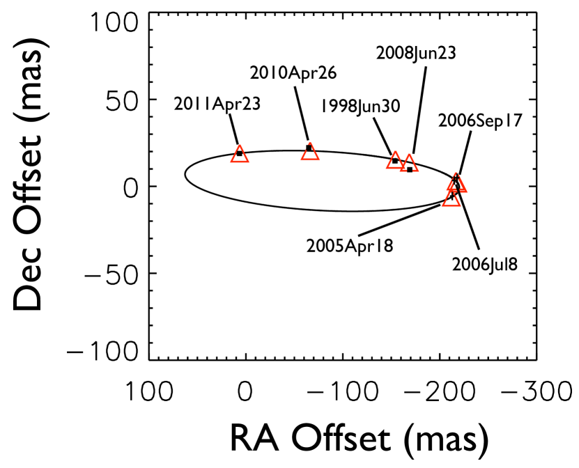
Figure 4.— The same as Figure 3, showing the orbital solution for the companion to HD 113449.

Figure 5.— The same as Figures 3 and 5, showing the orbital solution for the companion to HD 160934. Nominal error bars that are too small to be accurately represented are instead contained within filled squares.

Furthermore, in addition to our values presented in Table 6, relative astrometry measurements have been published by Hormuth et al. (2007) and Lafrenière et al. (2007). Using the combined data set, which is summarized in Table 9, we performed a least-squares orbital fit and report the results in Table 8. The solution is plotted in Figure 5. In order to achieve a reduced $\chi^{2}$ of 1.0, we had to add an extra position angle error of 0.4 degrees to all data, which may indicate a small position angle calibration mismatch between the three instruments used in this fit. Of these parameters, only $T_{0}$ has an uncertainty that would be significantly changed by the addition of radial velocity data, which have not been made available to us because at least one new paper including those data is in preparation (Montes, private communication). However, we can combine the semiamplitude of the radial velocity curve published in Griffin & Filiz Ak (2010) ($K_{1}$=7.39$\pm$0.22 km s^-1) with our orbital fit and the HIPPARCOS parallax of 30.2$\pm$2 mas (van Leeuwen, 2007) to obtain a mass of 0.48$\pm$0.06 $M_{\odot}$ for the companion. This value is consistent with the one derived above using isochrones, at the level of the uncertainties.

Although the binary orbit is not taken into account in computing the HIPPARCOS parallax, the period is several times longer than the length of the HIPPARCOS mission and the system was near apastron at the time of observations, so we do not expect the orbital photocenter motion to have a significant effect on the measured parallax. As the parallax uncertainty dominates our mass uncertainty, we have repeated the orbital calculation at several fixed parallax values as given in Table 10. According to the NextGen models of Baraffe et al. (1998), plausible ages for the companion range from $\sim$50 Myr through to the zero-age main sequence. Therefore, the dynamical mass does not allow us to place a strong constraint on the system age, but the lower range of allowed values is compatible with the age of AB Dor.

6.5. Survey Detection Limits

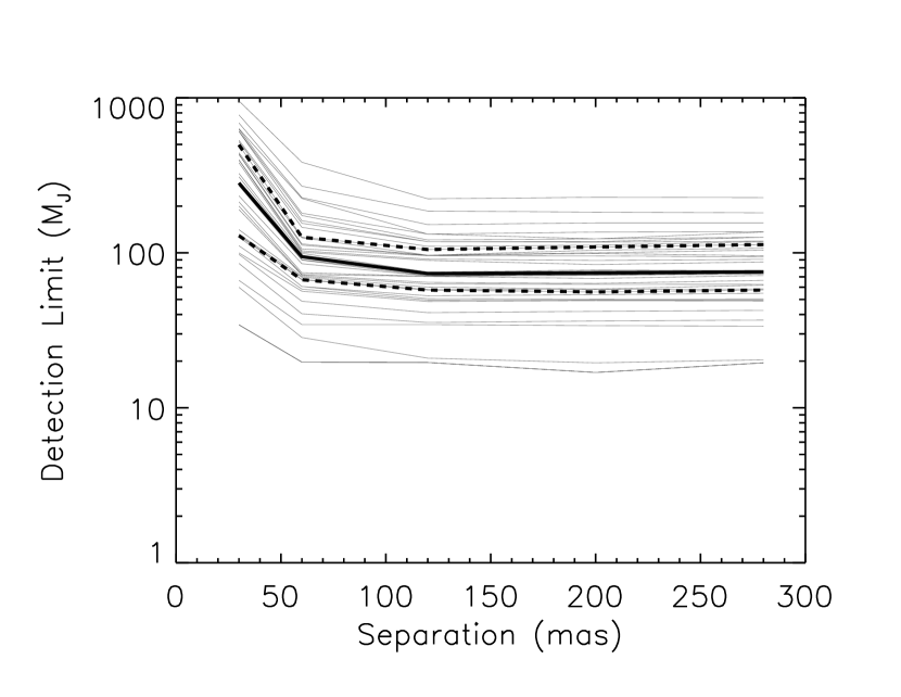
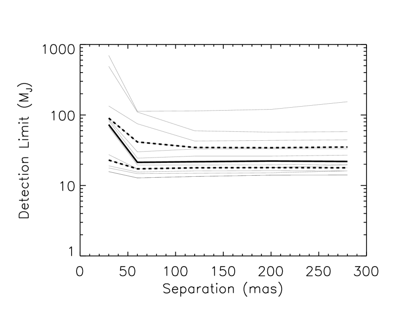
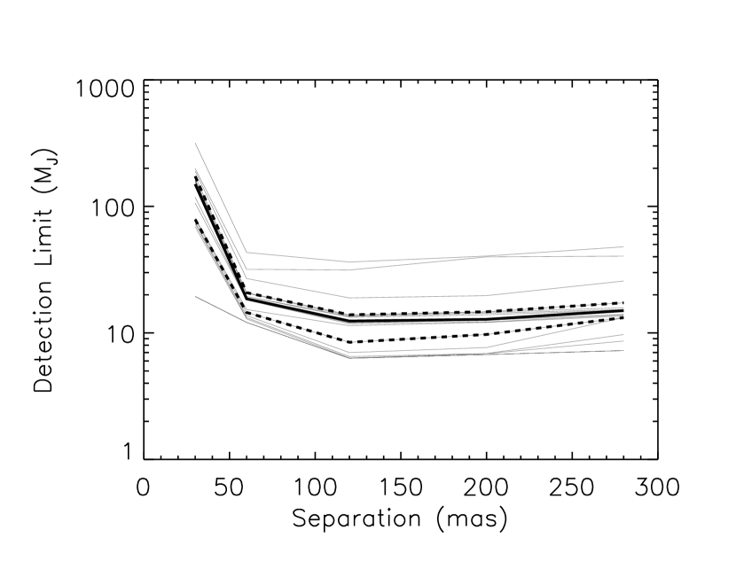
Figure 6.— Detection limits as a function of angular separation for the AB Dor and Her-Lyr targets (top), the $\beta$ Pic and Tuc-Hor targets (middle), and the TWA targets (bottom). In each plot, solid black lines show the median detection limits within the 20–40, 40–80, 80–160, 160–240, and 240–320 mas annuli, dashed black lines show the 25th and 75th percentiles, and solid gray lines show the individual detection limits.

We list our detection limits in Table 11, corresponding to the 99.9% threshold values for each of the separation annuli, as defined in Section 5. These were translated into upper limits for companion masses by first converting the contrast ratios into absolute companion magnitudes using the distances listed in Table 3. Then combining these intrinsic luminosities with the assumed ages listed in Table 2, we determined the corresponding companion mass by interpolating an appropriate set of isochrones: specifically, the DUSTY isochrones (Chabrier et al., 2000) for objects with $1400\,\rm{K}\,\lesssim T_{\rm{eff}}\lesssim 2800\,\rm{K}$ and the NextGen isochrones (Baraffe et al., 1998) for objects with $T_{\rm{eff}}\gtrsim 2800\,\rm{K}$. For the four targets with detected companions (HIP 14807, HD 16760, HD 113449, HD 160934) we quote the limits obtained for the residual closure phases.

It should be emphasized that the mass limits quoted in Table 11 inherit the systematic errors of the models used to compute them (eg. Baraffe et al., 2002). For instance, Marley et al. (2007) have shown that the predicted luminosities are highly dependent on the treatment of initial conditions, with “cold start” models generating luminosities that can be orders of magnitudes fainter than those obtained by the “hot start” DUSTY models over Gyr time scales. However, objects in the mass range that our survey is sensitive to would most likely have formed by the gravitational collapse of instabilities in the stellar disk, a process that is more akin to the hot start scenario. Indeed, recent observational evidence appears to favor the hot start models down to masses of $\sim$10$M_{\rm J}$ (eg. Lagrange et al., 2010) or even suggest that they could even overpredict the luminosity of such objects (Dupuy et al., 2009a, 2010). In the latter case, the values quoted in Table 11 would be conservative estimates.

With these considerations in mind, Figure 6 shows the detection limits plotted in terms of equivalent companion mass as a function of angular separation. Due to the heterogeneous nature of our observations, which were made using different instruments with different filters, we have divided the targets into three groups in these plots. The top panel shows the detection limits for our older AB Dor ($\sim$110 Myr) and Her-Lyr ($\sim$200 Myr) targets, the middle panel shows the detection limits for our younger $\beta$ Pic ($\sim$12 Myr) and Tuc-Hor ($\sim$30 Myr) targets, and the bottom panel shows the detection limits for the TWA ($\sim$8 Myr) targets. The TWA targets have been plotted on their own because all but three of them were observed during the same observing run at VLT using the L^′ filter with a 7-hole mask.

7. Substellar Companion Frequencies

We have used our detection limits listed in Table 11 to constrain the frequency of $\sim$ 20–80 $M_{\rm J}$ companions in $\sim$ 3–30 AU orbits around 0.2–1.5 $M_{\odot}$ stars. To do this, we employed the same methodology as Carson et al. (2006), Lafrenière et al. (2007), Nielsen et al. (2008), Metchev & Hillenbrand (2009), and Chauvin et al. (2010). We present a brief outline of the approach here, but the reader may consult those works for further details.

7.1. Mathematical Framework

Firstly, if we denote the outcome of our survey of $N_{s}$ stars as the set $\{d_{j}\}$, where $d_{j}$ is equal to zero if no companion was detected around the $j$th star or equal to one if a companion was detected, then the likelihood that the fraction of stars with companions is equal to $f$ is given by:

$$P\left(f|\{d_{j}\}\right) = \frac{\mathcal{L}\left(\{d_{j}\}|f\right)\,P(f)}{\int^{1}_{0}{\mathcal{L}\left(\{d_{j}\}|f\right)\,P(f)\,df}}$$ (5)

where $\mathcal{L}\left(\{d_{j}\}|f\right)$ is the likelihood of our data and $P(f)$ is the prior probability that the underlying companion frequency is equal to $f$. We adopt an ignorant prior of $P(f)=1$.

The fact that we did not detect any 20–80 $M_{\rm J}$ companions allows us to place an upper limit $f_{u}$ on their frequency by integrating Equation 5, such that:

$$\alpha = \frac{\int^{f_{u}}_{0}{\mathcal{L}\left(\{d_{j}\}|f\right)\,df}}{\int^{1}_{0}{\mathcal{L}\left(\{d_{j}\}|f\right)\,df}}$$ (6)

where $\alpha$ is a fraction giving the confidence of our limit (eg. $\alpha=0.95$ corresponds to a confidence of 95%).

Using Poisson statistics, it can be shown that a null result implies:

$$\mathcal{L}\left(\{d_{j}\}|f\right) = \prod^{N_{s}}_{j=1}{e^{-fp_{j}}}$$ (7)

where $p_{j}$ is the probability that a substellar companion would have been detected around the $j$th star if there had been one present.

7.2. Monte Carlo Analysis

The next task is to determine values for each of the $p_{j}$ terms, and we did this using a Monte Carlo (MC) approach. For each target star in our sample, we generated 10 000 hypothetical companions, each with a mass $M_{2}$ and angular separation $\rho$. The companion masses were either obtained by randomly sampling from an appropriate distribution (see Section 7.3 below) or else they were set to a fixed value (see Section 7.6 below). To obtain the angular separations, we had to properly take into account the companion orbital eccentricities, phases, and orientations. We did this using the approach described by Brandeker et al. (2006) in their Appendices 1 and 2. As with the companion masses, this required either randomly sampling these properties from appropriate distributions (see Sections 7.4 and 7.5 below) or else setting them to fixed values (see Section 7.6 below).

Having generated 10 000 hypothetical companions with masses and angular separations for each of the targets in our sample, we then consulted the detection limits in Table 11. Companions with masses that fell above the minimum detectable mass in the corresponding separation annulus for their target star were counted as detections. The $p_{j}$ value for each target was thus given by the number $x_{j}$ of such detections divided by the total number of hypothetical companions generated, i.e. $p_{j}=x_{j}/10\,000$. Equipped with the $p_{j}$ values, we were then able to calculate an estimate for the companion frequency upper limit $f_{u}$ at some level of confidence $\alpha$ by integrating Equation 6.

7.3. Mass Distributions

The distribution of substellar companion masses in the separation range $\sim$ 3–30 AU is not yet constrained by observations. To accomodate this uncertainty, we have repeated our MC analysis separately for three different assumed forms for the mass distribution. For the first of these, we extrapolated to 20–80 $M_{\rm J}$ the power law distribution that has been uncovered by the Keck radial velocity survey for companions with masses $M_{2}<10$ $M_{\rm J}$ and periods $P$ $<$ 2000 days (Cumming et al., 2008), given by:

$$\frac{d\mathcal{N}}{dM_{2}} \propto M_{2}^{-1.31}$$ (8)

where $d\mathcal{N}$ is the number of objects with masses in the interval $[M_{2},M_{2}+dM]$.

The second distribution that we used was the universal mass function proposed by Metchev & Hillenbrand (2009) for companions to solar mass stars, suggested by those authors for companion masses between 0.01 $M_{\odot}$ and 1.0 $M_{\odot}$ and semimajor axes between 0 AU and 1590 AU. It is given by:

$$\frac{d\mathcal{N}}{dq} \propto q^{-0.39}$$ (9)

where $q$ is the secondary-to-primary mass ratio.

The last distribution that we used was a log-normal paramaterization proposed by Kraus et al. (2008), derived using an ad hoc physical model of binary formation. It is given by:

$$\frac{d\mathcal{N}}{dq} \propto \frac{1}{q}\exp{\left[-\frac{1}{2}\left(\frac{\log_{10}q}{\sigma}\right)^{2}\right]}$$ (10)

and we used the authors’ proposed value of $\sigma=0.428$.

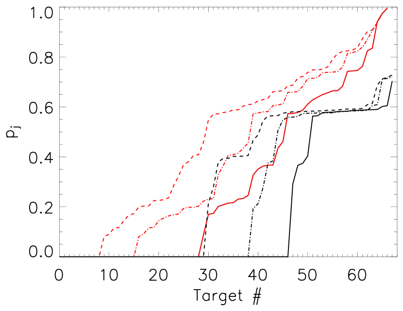
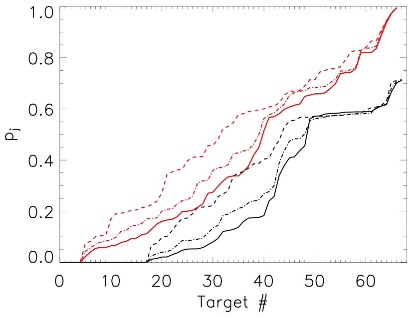
Figure 7.— Curves showing the $p_{j}$ values for the case of semimajor axes distributed according to $d\mathcal{N}/da\propto a^{-1}$ (Equation 12) and eccentricities distributed according to $d\mathcal{N}/de\propto 2e$ (Equation 11). The left panel shows the $p_{j}$ values obtained for fixed companion masses of 20 $M_{\rm J}$ (solid lines), 40 $M_{\rm J}$ (dash-dot lines), and 60 $M_{\rm J}$ (dashed lines), while the right panel shows the same values obtained for three assumed companion mass distributions: a mass power law given by Equation 8 (solid lines), a mass ratio power law given by Equation 9 (dash-dot lines), and a log-normal mass ratio parameterization given by Equation 10 (dashed lines). In both panels, the black curves indicate the values obtained using the aperture masking limits only, while the red curves show the equivalent values obtained when the imaging limits are also included (see Section 7.7). Note that for each curve, the values are arranged in ascending order so that, in general, a point on the horizontal axis does not correspond to the same target for all curves.

7.4. Eccentricity Distributions

As with masses, the distribution of substellar companion orbital eccentricities in the semimajor axis range $\sim$ 3–30 AU is not yet constrained by observations. We chose to draw companion eccentricities from a distribution of the form:

$$\frac{d\mathcal{N}}{de} \propto 2e$$ (11)

which, as noted in Appendix 2 of Brandeker et al. (2006), is an approximation that has been derived from physical considerations.

However, to test how sensitive our results were to the distribution of companion eccentricities, we repeated all of our MC analyses for two limiting cases: (1) fixing the orbital eccentricity of all hypothetical companions to $e=0.9$; (2) fixing all hypothetical companion eccentricities to $e=0$.

7.5. Semimajor Axis Distributions

We drew substellar companion semimajor axes from an inverse power law of the form:

$$\frac{d\mathcal{N}}{da} \propto a^{-1}$$ (12)

over the separation range 3–30 AU. This distribution was also used by Metchev & Hillenbrand (2009) for $a>30$ AU (see their Appendix 2 for a discussion) and it is consistent with recent results for stellar binaries between $\sim 5$–$500$ AU (eg. Kraus et al., 2008, 2011). Furthermore, in the event that $>$10 $M_{\rm J}$ objects can form by the same mechanism as lower-mass gas giant planets, Equation 12 is a reasonable extrapolation from the results of Cumming et al. (2008), who found a nearly-log-flat distribution for $<$10 $M_{\rm J}$ gas giant planets at separations $a<3$ AU.

7.6. Distribution-independent Approach

In addition to assuming specific forms for the distribution of companion properties, we repeated the analysis with them set to fixed values. This allowed us to obtain conservative upper limit estimates for the companion frequencies. For instance, the less massive a companion is, the more difficult it is to detect because it is fainter and hence the required contrasts are higher. Therefore, by setting all of our hypothetical substellar companions to have some mass $M^{\prime}_{2}$, the subsequent result we obtain from the MC analysis is an upper limit on the frequency of all companions with masses $M_{2}\geq M^{\prime}_{2}$.

Similarly, our ability to detect companions varied with angular separation (Figure 6), which is related to the semimajor axis of the companion via the distance to the system and the orientation of the orbit. Now suppose we fix the semimajor axes of the hypothetical companions to a certain value $a^{\prime}$ and repeat the MC analysis for values over some interval $a^{\prime}$ $\in$ $[a_{1},a_{2}]$. Then the maximum value of $f_{u}$ obtained from these analyses is the most conservative upper limit estimate for the frequency of companions with semimajor axes on that interval.

We present the results of these distribution-independent calculations in Section 7.9, as well as the results obtained by assuming the specific distribution forms described in Sections 7.3–7.5.

7.7. Previous Imaging Observations

Ideally, when performing the calculations described above, we would like to combine the results of our aperture masking survey with those of other imaging surveys targeting wider angular scales. This would allow us to put tighter constraints on the companion frequencies across a larger range of separations. To this end, we identified 49 of our targets that have previously been observed as part of published direct imaging surveys and list these in Table 12. For each of these targets, we quote the inner separation angle that was probed by the imaging observations as well as the corresponding sensitivity of the observations. In most cases, these values were taken directly from the published survey limits, but when these were not provided explicitly we attempted to make conservative estimates. We also list each of the sensitivities in Table 12 as an equivalent minimum detectable companion mass, calculated by interpolating the DUSTY isochrones of Chabrier et al. (2000) in the same manner outlined in Section 6.5. We incorporated these limits into our analysis described in Section 7.2 by treating hypothetical companions as “detected” (i.e. by increasing $x_{j}$ by 1) whenever they came within the detectability range of the previous imaging observations (i.e. if they had separation and masses above the values quoted in Table 12). In the next sections, we present the results obtained from this combined approach (aperture masking + previous imaging) together with the results obtained using the aperture masking limits alone.

7.8. Calculated $p_{j}$ Values

The $p_{j}$ values calculated separately for each of the three companion mass distributions that we considered (Equations 8, 9, and 10) are plotted in ascending order in Figure 7 for the case of a companion orbital eccentricity distribution given by $d\mathcal{N}/de\propto 2e$ (Equation 11) and semimajor axis distribution given by $d\mathcal{N}/da\propto a^{-1}$ (Equation 12). In this figure, we immediately see the advantage of combining our aperture masking results with the results from imaging surveys: the overall effect is roughly equivalent to an upwards shift of the $p_{j}$ values by $\sim$ 10–30% for the majority of targets.

7.9. Calculated $f_{u}$ Values

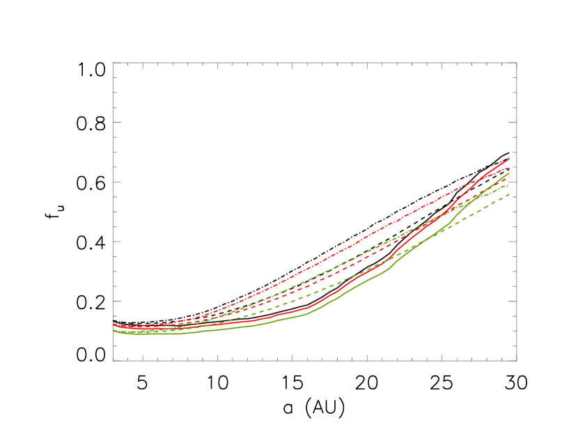
Figure 8.— 95% confidence $f_{u}$ estimates as a function of fixed companion semimajor axis obtained for the aperture masking limits alone with different assumptions about the companion eccentricities. The left panel shows values obtained for fixed companions masses of 20 $M_{\rm J}$ (black lines), 40 $M_{\rm J}$ (red lines), and 60 $M_{\rm J}$ (green lines). The right panel shows the same values obtained for companions distributed according to the mass power law given by Equation 8 (black lines), the mass ratio power law given by Equation 9 (red lines), and the log-normal mass ratio parameterization given by Equation 10 (green lines). In both panels, $f_{u}$ values are shown for the following cases: fixed companion eccentricities of $e=0$ (solid lines); fixed companion eccentricities of $e=0.9$ (dash-dot lines); and companion eccentricities randomly sampled from a distribution of the form $d\mathcal{N}/de\propto 2e$ (Equation 11) (dashed lines).

7.9.1 Assuming $d\mathcal{N}/da\propto a^{-1}$

In Table 13, we present 95% confidence (i.e. $\alpha=0.95$ in Equation 6) upper limit estimates $f_{u}$ for the frequency of 20–80 $M_{\rm J}$ substellar companions in the separation range 3–30 AU, with companion semimajor axes randomly drawn from the inverse power law distribution $d\mathcal{N}/da\propto a^{-1}$ (Equation 12). Also presented are calculations made separately for each permutation of the companion mass and eccentricity distributions described in Sections 7.3 and 7.4, respectively, as well as for different fixed companion masses of 20 $M_{\rm J}$, 40 $M_{\rm J}$, and 60 $M_{\rm J}$ (see Section 7.6).

All calculations reported in Table 13 are reasonably robust to the different assumptions made for the companion eccentricities, with the calculated upper limits only differing by $\lesssim$1–2% depending on whether all companion eccentricities are fixed to $e=0$ or $e=0.9$, or if they are drawn randomly from a distribution of the form $d\mathcal{N}/de\propto 2e$ (Equation 11). When the previous imaging observations are incorporated into the calculations and the ages and distances listed in Tables 2 and 3 are used, the upper limit estimates vary between 9–12%, depending on which form is assumed for the distribution of companion masses, but irrespective of what is assumed about the orbital eccentricities. When the previous imaging observations are not included in the analysis, the equivalent limits vary between 13–19%. For fixed companion masses of 20 $M_{\rm J}$, 40 $M_{\rm J}$ and 60 $M_{\rm J}$, the upper limit estimates vary between 15–16%, 11–12% and 9–10%, respectively, when the imaging observations are included, and between 25–27%, 18–20% and 14–15%, respectively, when the imaging observations are not included.

To investigate how sensitive our results are to the uncertainties in the distances and ages of our targets, we repeated the above calculations using the $1\sigma$ upper limits for the ages and distances of each target provided in Tables 2 and 3. For instance, instead of using a distance of 28 pc and an age of 110 Myr for PW And, we used $28+7=35$ pc and $110+40=150$ Myr, respectively. Assuming upper values for the ages and distances in this way results in a downward revision of our sensitivities to faint companions at smaller separations. Therefore, we had to re-calculate the survey detection limits presented in Table 11 before repeating the analysis described in Sections 7.2–7.7. Depending on which of the companion mass distributions is used, the upper limit estimates obtained from this analysis vary between 11–15% when the imaging observations are included, and between 17–24% when the imaging observations are not included. For fixed companion masses of 20 $M_{\rm J}$, 40 $M_{\rm J}$ and 60 $M_{\rm J}$, when the imaging observations are included the calculated upper limits vary between 20–23%, 14–15% and 11–12%, respectively, and when the imaging observations are not included they vary between 38–40%, 24–25% and 18–20%, respectively.

We also investigated how sensitive our results are to the 9 targets of less certain membership identified in Section 3 (i.e. HD 89744, HD 92945, GJ 466, EK Dra, HIP 30030, TWA-21, TWA-6, TWA-14, TWA-23) by removing them and the 7 Her-Lyr targets from the analysis. When all 16 of these targets are removed and we randomly sample the companion masses, the upper limit estimates vary between 12–15% when the imaging observations are included and between 16–23% when the imaging observations are not included, depending on which of the three companion mass distributions from Section 7.3 is used. For fixed companion masses of 20 $M_{\rm J}$, 40 $M_{\rm J}$ and 60 $M_{\rm J}$, the upper limit estimates vary between 18–20%, 14–15% and 12–13%, respectively, when the imaging observations are included, and between 31–32%, 22–23% and 17–19%, respectively, when the imaging observations are not included.

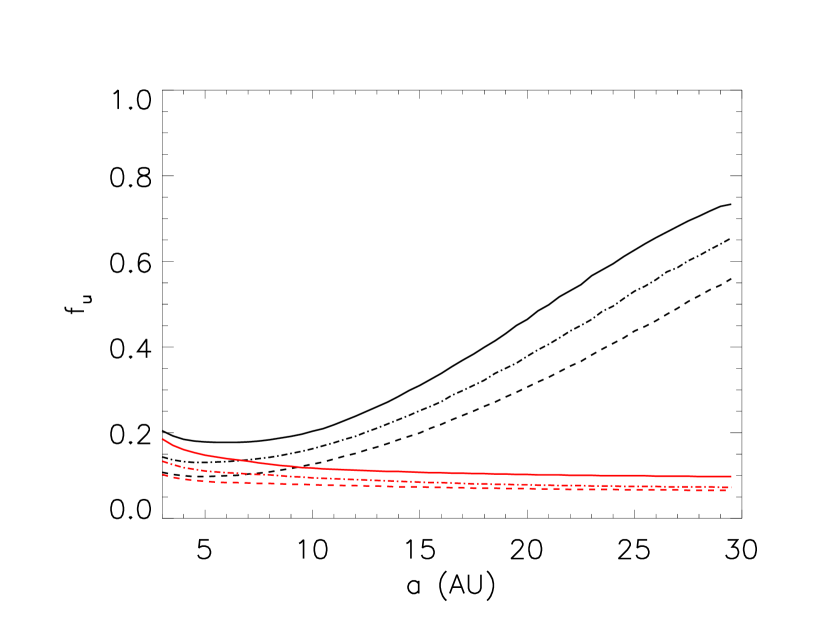
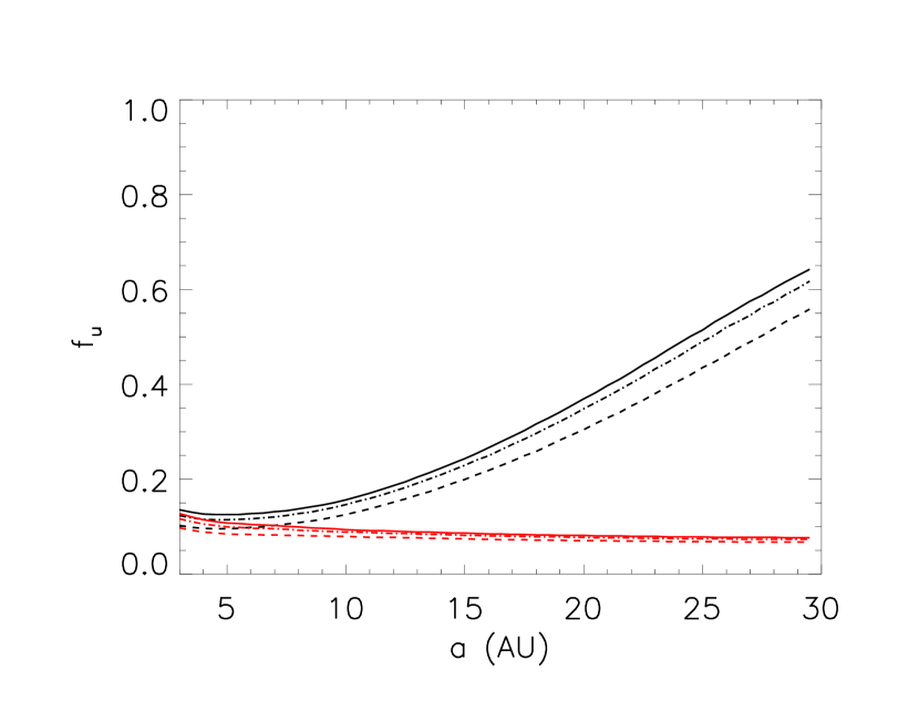
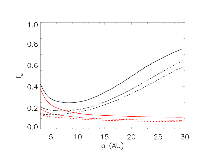
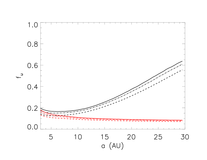
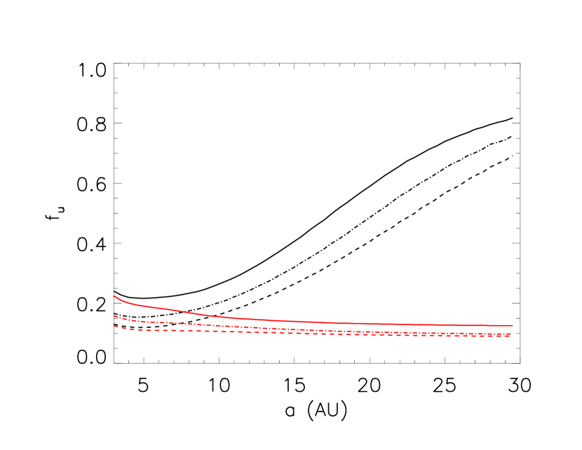
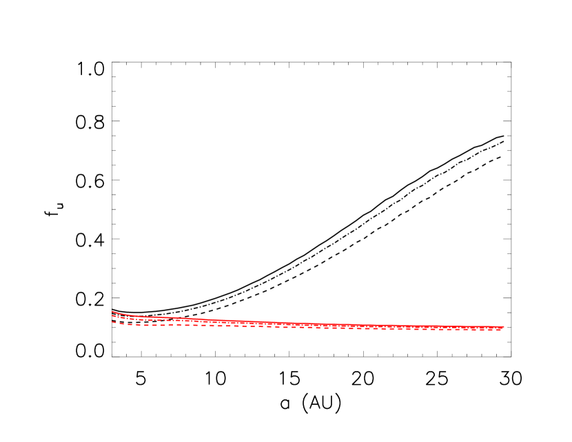
Figure 9.— 95% confidence $f_{u}$ estimates for companions with masses in the range 20–80 $M_{\rm J}$ as a function of fixed companion semimajor axes. As in Figure 7, the left panel shows the results for fixed companion masses and the right panel shows the results for companion masses drawn randomly from distributions. Colors and linestyles are the same as Figure 7.

Figure 10.— The same as Figure 11, but using values for the target distances and ages that give conservative estimates for the companion detection sensitivities. Specifically, the upper $1\sigma$ limits given in Tables 2 and 3 were used for the target ages and distances, respectively.

Figure 11.— The same as Figure 11, but excluding 16 of the targets whose moving group membership is not well-established; namely, the 9 targets that did not meet the ‘high probability’ criterion of Torres et al. (2008) in their dynamical convergence analysis (HD 89744, HD 92945, GJ 466, EK Dra, HIP 30030, TWA-21, TWA-6, TWA-14, TWA-23), and the 7 targets belonging to the proposed Her-Lyr moving group (see Section 3).

7.9.2 $d\mathcal{N}/da$ distribution–independent

We repeated all of the calculations presented in the previous section for fixed companion semimajor axes between 3–30 AU. As before, when the imaging observations were included in the analysis, the upper limit estimates only change by $\sim$1–2% over the entire 3–30 AU depending on which assumption is made for the companion eccentricities. However, when the aperture masking observations are used on their own this variation increases to $\sim$5–10% over the range 3–10 AU and becomes as high as $\sim$20% over the 10–30 AU range (Figure 8).

In Figure 11 we plot the calculated upper limit estimates obtained for fixed companion masses and randomly-sampled companion masses, while holding the semimajor axes fixed at successive values between 3–30 AU using a step size of 0.5 AU and randomly drawing the companion eccentricities from a distribution of the form $d\mathcal{N}/de\propto 2e$ (Equation 11). On their own, the aperture masking results place the tightest constraints over the $\sim$3–10 AU semimajor axis range, with upper limit estimates of 20%, 16% and 13% for fixed companion masses of 20 $M_{\rm J}$, 40 $M_{\rm J}$ and 60 $M_{\rm J}$, respectively. With the imaging observations included in the analysis, these limits improve to 19%, 13% and 10%, respectively. At larger separations between 10–30 AU, our upper limit estimates are 12%, 9%, and 8%, respectively, for the same companion masses when we include the imaging observations, while the companion frequencies are poorly constrained by the aperture masking observations alone.

Meanwhile, the right panel in Figure 11 shows the results that were obtained when we sampled the companion masses from each of the three distributions given in Section 7.3. Over the 10–30 AU semimajor axis range, the aperture masking observations on their own constrain the frequency of 20–80 $M_{\rm J}$ companions to be less than 16%, 15% or 13% at 95% confidence, depending on whether the mass power law (Equation 8), mass ratio power law (Equation 9) or mass ratio log-normal paramaterization (Equation 10) is assumed for the companions. These constraints improve to 13%, 12% and 10%, respectively, when the imaging observations are included in the analysis. At wider separations between 10–30 AU, the equivalent values obtained when the aperture masking observations are combined with the previous imaging observations are 9%, 9% and 8%, respectively.

Finally, Figures 11 and 11 have been included for completeness. They are the same as Figure 11 except that they show respectively the results obtained when upper values for the target ages and distances are used as described in Section 7.9.1, and the results obtained when the 9 targets of less certain membership identified in Section 3 and the Her-Lyr targets are not included in the calculations.

7.10. Implications for Formation Theories

A well-known result from radial velocity surveys is the discovery of a “brown dwarf desert” at separations $\lesssim$3 AU, where $\lesssim$0.5–1% of solar-like stars are found to possess a 13–75 $M_{\rm J}$ companion (Marcy & Butler, 2000; Grether & Lineweaver, 2006) compared with $\sim$10% possessing a 0.3–10 $M_{\rm J}$ companion (Cumming et al., 2008) and $\sim$13% possessing a $>$0.1 $M_{\odot}$ stellar companion (Duquennoy & Mayor, 1991). Meanwhile, at wider separations, imaging surveys have started to place upper limits on the frequency of substellar companions:

• Carson et al. (2006) obtained a 95% confidence upper limit of 12.1% on the frequency of 13–73 $M_{\rm J}$ companions between 25–100 AU.

• Lafrenière et al. (2007) obtained a 95% confidence interval of $1.9^{+8.3}_{-1.5}$% for the frequency of 13–75 $M_{\rm J}$ companions between 25–250 AU.

• Metchev & Hillenbrand (2009) obtained a 95% confidence interval of $3.2^{+7.3}_{-2.7}$% for the frequency of 13–75 $M_{\rm J}$ companions between 28–1590 AU. This is consistent with the results of Kraus et al. (2011), who obtained a lower bound of $3.9^{+2.6}_{-1.2}$% for the frequency of substellar companions over the range 5–5000 AU by combining the results of their aperture masking survey of Taurus-Auriga members with previous direct imaging results.

• By jointly analyzing the results from three of the largest and deepest surveys for substellar companions to date (Masciadri et al., 2005; Biller et al., 2007; Lafrenière et al., 2007), Nielsen & Close (2010) obtained 95% confidence upper limits of $<$20% and $<$5% for the frequency of companions with masses between 10–15 $M_{\rm J}$ in the ranges 13–600 AU and 40–200 AU, respectively.

The aperture masking survey reported in this paper has allowed us to place similar constraints on the frequency of 20–80 $M_{\rm J}$ companions over the 3–30 AU separation range (Sections 7.3–7.5).

These results are broadly in line with expectations from current models of substellar companion formation. Firstly, population synthesis models predict that core accretion only produces companions with masses up to $\sim$10 $M_{\rm J}$ (Ida & Lin, 2004), or else, if objects are formed with masses above 20 $M_{\rm J}$, then these are extremely rare (Mordasini et al., 2009). Unsurprisingly, the observational studies outlined above provide no evidence to the contrary, despite the aperture masking surveys in particular probing the range of separations where core accretion is expected to be most efficient.

Indeed, 20–80 $M_{\rm J}$ companions are much more likely to form by either gravoturbulent fragmentation during the initial collapse of the molecular cloud (eg. Bate, 2009; Offner et al., 2009) or by the fragmentation of gravitational instabilities in the protostellar disk once the initial free-fall collapse of the molecular cloud has ended (eg. Clarke, 2009; Stamatellos & Whitworth, 2009). For the gravoturbulent fragmentation scenario, the low frequencies of substellar companions deduced for separations $\lesssim$200 AU from observational studies is in qualitative agreement with the hydrodynamical simulations of Bate (2009) who found that the separation of binary pairs consisting of a stellar primary and a very low-mass secondary increases strongly with decreasing mass ratio. Meanwhile, the disk fragmentation mechanism is not expected to occur within $\sim$40–70 AU of the primary, where radiative cooling time scales are too long for the disk to be Toomre unstable (eg. Rafikov, 2007; Boley, 2009). Alternatively, 20–80 $M_{\rm J}$ objects might form by gravitational disk instabilities at separations beyond $\sim$40–70 AU and then migrate inwards. Stamatellos & Whitworth (2009) considered this for the case of a massive disk extending between 40–400 AU around a 0.7 $M_{\odot}$ star. However, they found that when low mass ($<$80 $M_{\rm J}$) companions did form at closer separations, they were subsequently scattered outwards by dynamical interactions with more massive companions in the same disk, leading to a brown dwarf desert that extended out to $\sim$100–200 AU. Again, the low occurence of 20–80 $M_{\rm J}$ companions inferred from observational studies over this separation range is consistent with such a scenario, though the constraints are not yet tight enough to make a definitive statement.

8. Conclusion

This paper has presented the results of an aperture masking survey of 67 young nearby stars for substellar companions. Our detection limits extend down to $\sim$ 40 $M_{\rm J}$ for 30 of our targets, and of these, we are sensitive down to $\sim$ 20 $M_{\rm J}$ or less for a subset of 22. Although we did not uncover any substellar companions, we detected four stellar companions. One of these, a $0.52\pm 0.09$ $M_{\odot}$ companion to HIP 14807, is a new discovery. We have also shown that the companion to HD 16760 is on a low inclination orbit with a mass of $0.28\pm 0.04$ $M_{\odot}$, much higher than the minimum mass of $M_{2}\,\sin i\sim$13–14 $M_{\rm J}$ inferred from radial velocity measurements.

If we do not make any assumptions about the distribution of companion masses or semimajor axes, we calculate that the frequency of 20–80 $M_{\rm J}$ companions is less than $\sim$ 19% in the range 3–10 AU and less than $\sim$ 12% in the range 10–30 AU at 95% confidence. If, however, we assume that the semimajor axes of 20–80 $M_{\rm J}$ companions are distributed according to $d\mathcal{N}/da\propto a^{-1}$ and that their masses are distributed according to a log-normal parameterization of the secondary-to-primary mass ratio, this limit becomes $\sim$9% over the 3–30 AU separation range. Similar values of $\sim$10% and $\sim$11% are obtained if we assume instead that the companion masses or secondary-to-primary mass ratios, respectively, are distributed according to power laws. These results are consistent with models that predict a low occurrence of substellar companions relative to stellar companions at these separations, possibly hinting at the extension of the brown dwarf desert beyond $\sim$ 3 AU.

Table 1Mask Properties

Observatory	Telescope	Instrument	Mask	Hole Diameter	Transmission
	Diameter (m)			(m)	%
Palomar	5.1	PHARO	9H	0.4	6
			18H	0.2	3
Keck	10	NIRC2	9H	1.1	11
			18H	0.5	5
VLT	8.2	CONICA	7H	1.2	15

Table 2Moving Groups Surveyed

Group	$N$	Age	Distance	Reference
		(Myr)	(pc)
AB Dor	31	$110\pm 40$	$34.1\pm 12.8$	Lu05, T08
$\beta$ Pic	11	$12\pm 5$	$34.5\pm 1.4$	Z01a, F06, T08
Her-Lyr	7	$200\pm 80$	$14.6\pm 4.1$	LS06
Tuc-Hor	2	$30\pm 10$	$45.1\pm 0.6$	Z01b, T08
TWA	16	$8\pm 4$	$55.0\pm 2.7$	dR06, T08

Table 3Sample List

Name	RA	DEC	Spectral	Mass	Distance	Ref.	K	H	J	Ref.	Membership	Previous
	(J2000)		Type	($M_{\odot}$)	(pc)		(mag)	(mag)	(mag)		Ref.	Imaging
AB Dor Targets
PW And	00 18 20.8	+30 57 24	K2	0.81	28 $\pm$ 7	ZS04	6.39	6.51	7.02	2M	ZS04, T08	MZ04, L05, L07,
												MH09, H10
HIP 3589	00 45 50.9	+54 58 40	F8	1.12	52.5 $\pm$ 2.5	HIP	6.69	6.72	6.93	2M	ZS04, T08	$\cdots$
HIP 5191	01 06 26.1	$-14$ 17 46	K1	0.86	47.3 $\pm$ 2.8	HIP	7.34	7.43	7.91	2M	ZS04, T08	C10
HIP 6276	01 20 32.2	$-11$ 28 03	G9	0.89	34.4 $\pm$ 1.2	HIP	6.55	6.65	7.03	2M	ZS04, T08	MH09
HIP 12635	02 42 20.9	+38 37 22	K2	0.79	50.4 $\pm$ 6.7	HIP	7.76	7.90	8.38	2M	ZS04, T08	$\cdots$
HD 16760	02 42 21.3	+38 37 08	G5	0.91	45.5 $\pm$ 4.9	HIP	7.11	7.15	7.47	2M	ZS04, T08	$\cdots$
HIP 13027	02 47 27.4	+19 22 19	G1	1.02	33.6 $\pm$ 0.9	HIP	6.05	6.10	6.37	2M	ZS04, T08	$\cdots$
HD 19668	03 09 42.3	$-09$ 34 47	G0	0.90	37.4 $\pm$ 1.6	HIP	6.70	6.79	7.16	2M	LS06, T08	MH09
HIP 14807	03 11 12.3	+22 25 24	K6	0.76	52.5 $\pm$ 8.6	HIP	7.96	8.10	8.67	2M	ZS04, T08	$\cdots$
HIP 14809	03 11 13.8	+22 24 58	G5	1.04	53.7 $\pm$ 3.3	HIP	6.97	7.07	7.27	2M	ZS04, T08	$\cdots$
HIP 16563A	03 33 13.5	+46 15 27	G5	0.88	34.4 $\pm$ 1.2	HIP	6.62	6.70	7.03	2M	ZS04, T08	B07
HIP 16563B	03 33 14.0	+46 15 19	M0	0.55	34.4 $\pm$ 1.2	HIP	8.07	8.21	8.83	2M	ZS04, T08	$\cdots$
HIP 17695	03 47 23.2	$-01$ 58 18	M3	0.46	16.1 $\pm$ 0.7	HIP	6.93	7.17	7.80	2M	ZS04, T08	L07
HIP 18859	04 02 36.7	$-00$ 16 06	F6	1.16	18.8 $\pm$ 0.1	HIP	4.18	4.34	4.71	2M	ZS04, T08	L07, H10
HIP 19183	04 06 41.5	+01 41 03	F5	1.17	55.2 $\pm$ 2.8	HIP	6.58	6.70	6.89	2M	ZS04, T08	$\cdots$
BD+20 1790	07 23 44.0	+20 25 06	K5	0.76	32 $\pm$ 8	LS06	6.88	7.03	7.64	2M	LS06, T08	L05, MH09, H10
HD 89744	10 22 10.6	+41 13 46	F7	1.52	39.4 $\pm$ 0.5	HIP	4.45	4.53	4.86	2M	LS06	$\cdots$
HIP 51317	10 28 55.6	+00 50 28	M2	0.43	7.1 $\pm$ 0.1	HIP	5.31	5.61	6.18	2M	LS06, T08	M05, L07
HD 92945	10 43 28.3	$-$29 03 51	K1	0.85	21.4 $\pm$ 0.3	HIP	5.66	5.77	6.18	2M	LS06	B07, L07
GJ 466	12 25 58.6	+08 03 44	M0	0.73	37.4 $\pm$ 3.2	HIP	7.33	7.45	8.12	2M	LS06	MZ04
HD 113449	13 03 49.8	$-05$ 09 41	K1	0.84	21.7 $\pm$ 0.4	HIP	5.72	5.89	6.27	2M	ZS04, T08	L07, H10
EK Dra	14 39 00.2	+64 17 30	G1.5	1.06	34.1 $\pm$ 0.4	HIP	5.91	6.01	6.32	2M	LS06	MZ04, B07, L07,
												MH09
HIP 81084	16 33 41.7	$-09$ 33 10	M0	0.58	30.7 $\pm$ 2.3	HIP	7.55	7.78	8.38	2M	ZS04, T08	L07
HIP 82688	16 54 08.2	$-04$ 20 24	G0	1.12	46.7 $\pm$ 2.0	HIP	6.36	6.48	6.70	2M	ZS04, T08	MH09
HD 160934	17 38 39.7	+61 14 16	K7	0.70	33.1 $\pm$ 2.2	HIP	7.22	7.37	7.98	2M	ZS04, T08	L05, H07, L07,
												MZ04
HIP 106231	21 31 01.6	+23 20 09	K5	0.75	24.8 $\pm$ 0.7	HIP	6.38	6.52	7.08	2M	ZS04, T08	L05, L07, MZ04
HIP 110526	22 23 29.1	+32 27 34	M3	0.48	15.5 $\pm$ 1.6	HIP	6.05	6.28	6.90	2M	ZS04, T08	$\cdots$
HIP 113579	23 00 19.2	$-26$ 09 12	G5	0.99	30.8 $\pm$ 0.7	HIP	5.94	6.04	6.29	2M	ZS04, T08	MH09, C10
HIP 114066	23 06 04.6	+63 55 35	M1	0.60	24.5 $\pm$ 1.0	HIP	6.98	7.17	7.82	2M	ZS04, T08	L07
HIP 115162	23 19 39.5	+42 15 10	G4	0.94	50.2 $\pm$ 2.9	HIP	7.22	7.28	7.61	2M	ZS04, T08	$\cdots$
HIP 118008	23 56 10.5	$-39$ 03 07	K2	0.81	22.0 $\pm$ 0.4	HIP	5.91	6.01	6.51	2M	ZS04, T08	B07, C10
$\beta$ Pic Targets
HR9	00 06 50.1	$-23$ 06 27	F3	1.40	39.4 $\pm$ 0.6	HIP	5.24	5.33	5.45	2M	ZS04, T08	K03
HIP 10680	02 17 25.2	+28 44 43	F5	1.15	34.5 $\pm$ 0.6	HIP	5.79	5.84	6.05	2M	ZS04, T08	$\cdots$
HIP 11437B	02 27 28.1	+30 58 41	M2	0.35	40.0 $\pm$ 3.6	HIP	7.92	8.14	8.82	2M	ZS04, T08	$\cdots$
HIP 11437A	02 27 29.2	+30 58 25	K6	0.63	40.0 $\pm$ 3.6	HIP	7.08	7.24	7.87	2M	ZS04, T08	$\cdots$
HIP 12545	02 41 25.8	+05 59 19	K6	0.67	42.0 $\pm$ 2.7	HIP	7.07	7.23	7.9	2M	ZS04, T08	B07
51 Eri	04 37 36.1	$-02$ 28 25	F0	1.41	29.4 $\pm$ 0.3	HIP	4.54	4.77	4.74	2M	ZS04, T08	H10
HIP 25486	05 27 04.8	$-11$ 54 04	F7	1.25	27.0 $\pm$ 0.4	HIP	4.93	5.09	5.27	2M	ZS04, T08	L05, K07, MH09
GJ 803	20 45 09.5	$-31$ 20 27	M1	0.44	9.9 $\pm$ 0.1	HIP	4.53	4.83	5.44	2M	ZS04, T08	K03, MZ04, M05,
												B07, L07
BD$-$17 6128	20 56 02.7	$-17$ 10 54	K6	0.73	45.7 $\pm$ 1.6	HIP	7.12	7.25	7.92	K04	ZS04, T08	M05
HIP 112312A	22 44 57.9	$-33$ 15 02	M4	0.31	23.3 $\pm$ 2.0	HIP	6.93	7.15	7.79	2M	ZS04, T08	B07
HIP 112312B	22 45 00.0	$-33$ 15 26	M4.5	0.17	23.3 $\pm$ 2.0	HIP	7.79	8.06	8.68	2M	ZS04, T08	$\cdots$
Her-Lyr Targets
HD 166	00 06 36.8	29 01 17.4	K0	0.93	13.7 $\pm$ 0.1	HIP	4.31	4.63	4.73	2M	LS06	L07, H10
HD 10008	01 37 35.5	-06 45 37.5	G5	0.89	24.0 $\pm$ 0.4	HIP	5.75	5.90	6.23	2M	LS06	L07
HD 233153	05 41 30.7	+53 29 23	M0.5	0.58	12.4 $\pm$ 0.3	HIP	5.76	5.96	6.59	2M	LS06	C05
HIP 37288	07 39 23.0	+02 11 01	K7	0.61	14.6 $\pm$ 0.3	HIP	5.87	6.09	6.77	2M	LS06	M05, L07
HD 70573	08 22 50.0	01 51 33.6	G6	0.89	46 $\pm$ 11	LS06	7.19	7.28	7.56	2M	LS06	L05, MH09
HIP 53020	10 50 52.1	+06 48 29	M4	0.25	6.8 $\pm$ 0.2	HIP	6.37	6.71	7.32	2M	LS06	L07
HN Peg	21 44 31.3	+14 46 19	G0	1.06	17.9 $\pm$ 0.1	HIP	4.56	4.6	4.79	2M	LS06	MZ04, L07
Tuc-Hor Targets
HIP 9141	01 57 48.9	$-21$ 54 05	G4	0.97	40.9 $\pm$ 1.1	HIP	6.47	6.56	6.86	2M	ZS04, T08	B07, MH09
HIP 30030	06 19 08.1	$-03$ 26 20	G0	1.03	49.2 $\pm$ 2.0	HIP	6.55	6.59	6.85	2M	ZS04	B07, MH09
TWA Targets
TWA-21	10 13 14.8	$-52$ 30 54	K3/4	0.63	48 $\pm$ 4	MM05	7.19	7.35	7.87	2M	ZS04	$\cdots$
TWA-6	10 18 28.8	$-31$ 50 02	K7	0.43	55 $\pm$ 5	MM05	8.04	8.18	8.87	2M	ZS04	W99, MZ04, L05,
												M05
TWA-7	10 42 30.3	$-33$ 40 17	M2	0.35	29 $\pm$ 2	MM05	6.9	7.13	7.79	2M	ZS04, T08	W99, MZ04, L05
TW Hya	11 01 51.9	$-34$ 42 17	K6	0.64	53.7 $\pm$ 6.2	HIP	7.30	7.56	8.22	2M	ZS04, T08	W99, MZ04, L05
TWA-3	11 10 28.0	$-37$ 31 53	M4	0.37	36 $\pm$ 4	MM05	7.28	7.60	$\cdots$	W00	ZS04, T08	W99, C10
TWA-14	11 13 26.5	$-45$ 23 43	M0	0.57	86 $\pm$ 8	MM05	8.50	8.73	9.42	2M	ZS04	B07, MZ04, C10
TWA-13B	11 21 17.2	$-34$ 46 45	M1	0.63	57 $\pm$ 10	MM05	7.49	7.73	8.43	2M	ZS04, T08	$\cdots$
TWA-13A	11 21 17.5	$-34$ 46 50	M1	0.61	57 $\pm$ 10	MM05	7.46	7.68	8.43	2M	ZS04, T08	$\cdots$
TWA-8B	11 32 41.4	$-26$ 52 08	M5	0.14	42 $\pm$ 5	MM05	9.01	9.36	$\cdots$	W00	ZS04, T08	W99, M05, L05
TWA-8A	11 32 41.5	$-26$ 51 55	M3	0.40	41 $\pm$ 4	MM05	7.44	7.72	$\cdots$	W00	ZS04, T08	W99, M05
TWA-9	11 48 24.2	$-37$ 28 49	K5	0.38	46.8 $\pm$ 5.4	HIP	7.85	8.03	8.68	2M	ZS04, T08	W99, M05
TWA-23	12 07 27.4	$-32$ 47 00	M1	0.58	61 $\pm$ 5	MM05	7.75	8.03	8.62	2M	ZS04	C10
TWA-25	12 15 30.8	$-39$ 48 42	M1	0.68	55 $\pm$ 4	MM05	7.31	7.50	8.17	2M	ZS04, T08	B07, C10
TWA-10	12 35 04.3	$-41$ 36 39	M2	0.39	57 $\pm$ 9	MM05	8.19	8.48	9.12	2M	ZS04, T08	W99, MZ04, L05
TWA-11B	12 36 00.6	$-39$ 52 16	M2	0.52	72.8 $\pm$ 1.7	HIP	8.35	8.53	9.15	2M	ZS04, T08	W99
TWA-11A	12 36 01.0	$-39$ 52 10	A0	2.31	72.8 $\pm$ 1.7	HIP	5.77	5.79	5.78	2M	ZS04, T08	W99, C10

Table 4Filters Used

Instrument	Filter	$\lambda_{0}$ ($\mu$m)	$\Delta\lambda$ ($\mu$m)
PHARO	CH4s	1.57	0.10
	H	1.64	0.30
	Ks	2.15	0.31
NIRC2	Jcont	1.21	0.02
	Hcont	1.58	0.02
	CH4s	1.59	0.13
	Kp	2.12	0.35
	Kcont	2.27	0.03
	CO	2.29	0.03
CONICA	L′	3.80	0.62

Table 5Observations

Target	Instrument	Filter	Mask	$T_{\rm int}$ (min)	Date	MJD
AB Dor Targets
PW And	PHARO	CH4s	18H	3.9	2007 Jun 01	54252.5
HIP 3589	PHARO	CH4s	9H	6.5	2007 Nov 27	54431.1
HIP 5191	NIRC2	Hcont	18H	4.0	2007 Jun 06	54257.6
HIP 6276	NIRC2	Kcont	18H	5.3	2007 Nov 23	54427.2
HIP 12635	NIRC2	Kcont	18H	800	2008 Dec 23	54823.2
HD 16760	NIRC2	Kcont	18H	2.7	2008 Dec 23	54823.2
	NIRC2	Kcont	18H	13	2009 Aug 06	55049.6
	NIRC2	Jcont	18H	2.7	2009 Nov 20	55155.3
	NIRC2	Hcont	18H	2.7	2009 Nov 20	55155.3
	NIRC2	Kcont	18H	2.7	2009 Nov 20	55155.3
	NIRC2	CO	18H	2.7	2009 Nov 21	55156.2
HIP 13027	PHARO	Ks	9H	19	2007 Nov 27	54431.2
HD 19668	PHARO	Ks	9H	5.8	2007 Nov 29	54433.3
HIP 14807	PHARO	Ks	9H	5.8	2007 Nov 29	54433.1
	NIRC2	CO	18H	5.0	2009 Nov 21	55156.2
HIP 14809	NIRC2	CO	18H	2.7	2009 Nov 21	55156.2
HIP 16563A	PHARO	Ks	9H	5.8	2007 Nov 27	54431.3
HIP 16563B	NIRC2	CO	18H	5.3	2009 Nov 21	55156.2
HIP 17695	PHARO	Ks	9H	12	2007 Nov 29	54433.3
HIP 18859	PHARO	Ks	9H	8.7	2007 Nov 27	54431.2
HIP 19183	PHARO	Ks	9H	8.7	2007 Nov 27	54431.3
BD+20 1790	PHARO	Ks	9H	5.8	2007 Nov 27	54431.5
HD 89744	PHARO	CH4s	18H	8.6	2007 Apr 05	54195.3
HIP 51317	PHARO	Ks	9H	13	2007 Apr 06	54196.3
HD 92945	NIRC2	Kcont	18H	1.3	2007 Jun 06	54257.2
GJ 466	PHARO	Ks	9H	2.2	2008 Jun 19	54636.2
HD 113449	PHARO	CH4s	18H	13	2007 Apr 06	54196.3
	PHARO	Ks	9H	7.5	2007 Apr 07	54197.4
	PHARO	CH4s	18H	3.9	2007 Jun 01	54252.1
	NIRC2	Hcont	18H	1.3	2008 Jun 17	54634.2
	NIRC2	CH4s	9H	1.7	2008 Dec 21	54821.7
	NIRC2	Hcont	18H	2.7	2010 Apr 25	55311.4
EK Dra	PHARO	Ks	9H	4.3	2008 Jun 20	54637.2
HIP 81084	PHARO	CH4s	18H	4.3	2007 May 30	54250.2
HIP 82688	PHARO	CH4s	18H	4.3	2007 Jun 02	54253.4
HD 160934	PHARO	H	9H	9.7	2008 Jun 23	54640.3
	PHARO	Ks	9H	8.6	2008 Jun 23	54640.3
	NIRC2	Kcont	Clear	0.2	2010 Apr 26	55312.6
	NIRC2	Jcont	18H	2.7	2011 Apr 23	55674.6
	NIRC2	Hcont	18H	2.7	2011 Apr 23	55674.6
HIP 106231	PHARO	CH4s	18H	4.8	2007 May 31	54251.4
HIP 110526	PHARO	CH4s	9H	1.9	2007 May 31	54251.4
HIP 113579	NIRC2	Hcont	18H	2.7	2007 Jun 05	54256.6
HIP 114066	PHARO	CH4s	18H	3.9	2007 Jun 01	54252.4
HIP 115162	NIRC2	Kcont	18H	5.3	2009 Nov 21	55156.2
HIP 118008	NIRC2	Kcont	18H	5.3	2007 Nov 23	54427.2
$\beta$ Pic Targets
HR9	NIRC2	Hcont	18H	2.7	2007 Jun 06	54257.6
HIP 10680	NIRC2	Kcont	18H	5.3	2007 Nov 24	54428.4
HIP 11437A	NIRC2	Kcont	18H	5.3	2007 Nov 24	54428.4
HIP 11437B	NIRC2	Kcont	18H	5.3	2007 Nov 24	54428.4
HIP 12545	NIRC2	Kcont	18H	5.3	2007 Nov 24	54428.4
51 Eri	NIRC2	Kcont	18H	5.3	2008 Dec 21	54821.4
HIP 25486	PHARO	Ks	9H	12	2007 Nov 27	54431.4
GJ 803	NIRC2	Hcont	18H	4.0	2007 Jun 05	54256.5
BD$-$17 6128	PHARO	CH4s	9H	4.3	2007 May 30	54250.5
HIP 112312A	NIRC2	Kp	9H	10	2008 Jun 17	54634.6
HIP 112312B	NIRC2	Hcont	18H	2.7	2007 Jun 05	54256.6
Her-Lyr Targets
HD 166	PHARO	CH4s	18H	5.8	2007 May 31	54251.5
HD 10008	NIRC2	Kcont	18H	5.3	2007 Nov 23	54427.3
HD 233153	PHARO	Ks	9H	8.7	2007 Nov 27	54431.5
HIP 37288	NIRC2	Kcont	18H	5.3	2007 Nov 24	54428.6
HD 70573	PHARO	Ks	9H	13	2007 Nov 27	54431.5
HIP 53020	NIRC2	Kcont	18H	2.3	2007 Jun 06	54257.3
HN Peg	PHARO	CH4s	18H	3.9	2007 Jun 01	54252.5
Tuc-Hor Targets
HIP 9141	PHARO	Ks	9H	9.7	2007 Nov 29	54433.2
HIP 30030	NIRC2	Kcont	18H	5.3	2007 Nov 24	54428.6
TWA Targets
TWA-21	CONICA	L′	7H	20	2009 Mar 06	54896.1
TWA-6	CONICA	L′	7H	20	2009 Mar 07	54897.1
TWA-7	CONICA	L′	7H	40	2009 Mar 06	54896.1
TW Hya	CONICA	L′	7H	60	2009 Mar 07	54897.2
TWA-3	NIRC2	Kp	9H	11	2008 Dec 22	54822.7
TWA-14	CONICA	L′	7H	20	2009 Mar 07	54897.1
TWA-13B	NIRC2	Kp	9H	5.3	2008 Dec 21	54821.6
TWA-13A	CONICA	L′	7H	40	2009 Mar 06	54896.2
TWA-8B	NIRC2	Kp	9H	5.3	2008 Dec 23	54823.7
TWA-8A	CONICA	L′	7H	20	2009 Mar 05	54895.3
TWA-9	CONICA	L′	7H	20	2009 Mar 05	54895.3
TWA-23	CONICA	L′	7H	25	2009 Mar 05	54895.3
TWA-25	CONICA	L′	7H	20	2009 Mar 06	54896.2
TWA-10	CONICA	L′	7H	20	2009 Mar 06	54896.3
TWA-11B	CONICA	L′	7H	20	2009 Mar 07	54897.3
TWA-11A	CONICA	L′	7H	50	2009 Mar 07	54897.4

Table 6Detected Companions

Primary	Instrument	Date	MJD	Filter	$\lambda_{0}$ ($\mu m$)	$\rho$ (mas)	$\theta$ (deg)	$C$	$M_{2}$ ($M_{\odot}$)
HIP14807	PHARO	2007 Nov 29	54433.1	Ks	2.15	$63.22$	$246.86$	$10.15$	$\cdots$
	NIRC2	2009 Nov 21	55156.2	CO	2.29	$28.74\pm 0.19$	$89.74\pm 0.29$	$3.00\pm 0.06$	$0.52\pm 0.09$
HD16760	NIRC2	2008 Dec 23	54823.2	Kcont	2.27	$26.11\pm 2.59$	$46.20\pm 1.26$	$13.48\pm 3.15$	$0.32\pm 0.11$
	NIRC2	2009 Aug 6	55049.6	Kcont	2.27	$26.78\pm 0.90$	$204.54\pm 0.45$	$13.11\pm 1.00$	$0.32\pm 0.09$
	NIRC2	2009 Nov 20	55155.3	Jcont	1.21	$28.13\pm 1.93$	$286.50\pm 3.62$	$31.04\pm 5.92$	$0.24\pm 0.08$
	NIRC2	2009 Nov 20	55155.3	Hcont	1.58	$26.06\pm 1.75$	$286.87\pm 1.94$	$20.53\pm 1.88$	$0.27\pm 0.08$
	NIRC2	2009 Nov 20	55155.3	Kcont	2.27	$39.07$	$286.67$	$26.58$	$\cdots$
	NIRC2	2009 Nov 21	55156.2	CO	2.29	$25.37\pm 4.51$	$290.25\pm 1.95$	$15.18\pm 6.44$	$0.29\pm 0.15$
HD113449	PHARO	2007 Apr 6	54196.3	CH4s	1.57	$35.62\pm 0.51$	$225.19\pm 0.44$	$4.27\pm 0.25$	$0.51\pm 0.02$
	PHARO	2007 Apr 7	54197.4	Ks	2.15	$40.46$	$223.30$	$6.68$	$\cdots$
	PHARO	2007 Jun 1	54252.1	CH4s	1.57	$28.46$	$179.92$	$13.73$	$\cdots$
	NIRC2	2008 Jun 17	54634.2	Hcont	1.58	$36.68\pm 0.13$	$222.91\pm 0.21$	$4.65\pm 0.05$	$0.50\pm 0.02$
	NIRC2	2008 Dec 21	54821.7	CH4s	1.59	$27.87\pm 0.13$	$250.14\pm 0.18$	$4.62\pm 0.03$	$0.51\pm 0.03$
	NIRC2	2010 Apr 25	55311.4	Hcont	1.58	$35.81\pm 0.17$	$202.38\pm 0.23$	$4.58\pm 0.06$	$0.51\pm 0.02$
HD160934	PHARO	2008 Jun 23	54640.3	H	1.64	$169.24\pm 0.13$	$273.35\pm 0.05$	$2.22\pm 0.01$	$0.54\pm 0.03$
	PHARO	2008 Jun 23	54640.3	Ks	2.15	$169.79\pm 0.25$	$273.29\pm 0.09$	$2.11\pm 0.02$	$0.54\pm 0.04$
	NIRC2	2010 Apr 26	55312.6	Kcont	2.27	$68.8\pm 0.7$	$290.0\pm 0.6$	$2.1\pm 0.2$	$0.54\pm 0.04$
	NIRC2	2011 Apr 23	55674.6	Jcont	1.21	$19.96\pm 0.05$	$18.44\pm 0.12$	$2.21\pm 0.01$	$0.54\pm 0.03$
	NIRC2	2011 Apr 23	55674.6	Hcont	1.58	$20.00\pm 0.03$	$18.42\pm 0.09$	$2.18\pm 0.01$	$0.54\pm 0.03$

Table 7Revised Fits For Degenerate Solutions

					Prior	Refitted Solution
Primary	Instrument	Date	MJD	Filter	$C$	$C$	$\rho$ (mas)	$\theta$ (deg)
HIP14807	PHARO	2007 Nov 29	54433.1	Ks	$3.00\pm 0.06$	$3.00\pm 0.06$	$45.43\pm 1.15$	$248.08\pm 2.30$
HD16760	NIRC2	2009 Nov 20	55155.3	Kcont	$13.19\pm 0.94$	$14.05\pm 0.92$	$25.80\pm 1.03$	$287.99\pm 1.89$
HD113449	PHARO	2007 Jun 01	54252.1	CH4s	$4.62\pm 0.02$	$4.62\pm 0.02$	$21.97\pm 0.73$	$179.96\pm 2.84$

Table 8System parameters for binaries with orbits

	HD 16760	HD 113449	HD 160934
$P$ (days)	$466.5\pm 0.4$	$216.9\pm 0.2$	$3764.0\pm 12.4$
$T_{0}$ (MJD)	$53336.5\pm 3$	$53410.5\pm 1$	$52389.5\pm 64$
$e$	$0.084\pm 0.003$	$0.300\pm 0.005$	$0.636\pm 0.020$
$i$ (deg)	$2.6\pm 0.5$	$57.5\pm 1.5$	$82.3\pm 0.8$
$a$ (mas)	$25.5\pm 2.8$	$33.7\pm 0.4$	$152.5\pm 4.7$
$a$ (AU)	$1.16\pm 0.18$	$0.73\pm 0.02$	$5.05\pm 0.37$
$\Omega$ (deg)	$86.9\pm 1.1$	$201.8\pm 1.6$	$266.7\pm 0.6$
$\omega$ (deg)	$243\pm 2$	$114.5\pm 0.5$	$216.0\pm 3.1$
$M_{\rm{total}}$ ($M_{\odot}$)	$0.96\pm 0.44$	$1.10\pm 0.09$	$1.21\pm 0.27$

Table 9HD 160934B Astrometry

Date	MJD	$\rho$ (mas)	$\theta$ (deg)	Source
1998 Jun 30	50994	$155\pm 1$	$275.5\pm 0.2$	Hormuth et al. (2007)
2005 Apr 18	53478.9	$213\pm 2$	$268.5\pm 0.7$	Lafrenière et al. (2007)
2006 Jul 8	53924	$215\pm 2$	$270.9\pm 0.3$	Hormuth et al. (2007)
2006 Sep 17	53995.2	$218\pm 2$	$271.3\pm 0.7$	Lafrenière et al. (2007)
2008 Jun 23	54640.3	$169.4\pm 0.3$	$273.3\pm 0.1$	This study
2010 Apr 26	55312.6	$68.8\pm 0.7$	$290.0\pm 0.6$	This study
2011 Apr 23	55674.6	$20.0\pm 0.1$	$18.43\pm 0.1$	This study

Table 10HD 160934B at fixed parallax

$\pi$	Mass	$K$	Model Age
(mas)	(M⊙)	(mag)	(Myr)
28.2	0.603$\pm$0.042	5.29$\pm$0.02	$\gtrsim$100
30.2	0.526$\pm$0.037	5.44$\pm$0.02	100${}^{+100}_{-50}$
32.3	0.463$\pm$0.032	5.59$\pm$0.02	55$\pm$10

Table 11Survey Detection Limits

			Detection limits for each separation annulus
				$\Delta\,m$ (mag)						$M_{2}$ ($M_{J}$)
Target	Instrument	Filter		20–40	40–80	80–160	160–240	240–320		20–40	40–80	80–160	160–240	240–320
AB Dor Targets
PW And	PHARO	CH4s		2.27	4.52	4.81	4.74	4.73		381	99	91	95	96
HIP 3589	PHARO	CH4s		3.23	5.31	5.60	5.54	5.57		443	125	105	109	107
HIP 5191	NIRC2	Hcont		4.56	4.84	4.79	4.73	4.23		111	103	96	100	136
HIP 6276	NIRC2	Kcont		4.07	5.33	5.25	5.22	5.21		141	72	75	76	77
HIP 12635	NIRC2	Kcont		3.85	4.93	4.88	4.81	4.83		127	73	75	78	77
HD 16760	NIRC2	Kcont		5.16	6.20	6.17	6.13	6.13		85	49	50	50	50
HIP 13027	PHARO	Ks		1.53	4.38	5.30	5.42	5.39		606	155	96	89	91
HD 19668	PHARO	Ks		0.960	4.05	4.99	5.09	5.03		609	146	89	84	87
HIP 14807	NIRC2	CO		3.98	5.20	5.12	5.09	5.08		132	70	73	74	74
HIP 14809	NIRC2	CO		3.84	4.95	4.91	4.84	4.80		233	114	118	123	126
HIP 16563A	PHARO	Ks		2.02	4.71	5.66	5.72	5.67		442	101	58	56	58
HIP 16563B	NIRC2	CO		4.12	5.26	5.19	5.15	5.13		60	34	36	36	37
HIP 17695	PHARO	Ks		0.52	3.71	4.74	4.77	4.78		275	57	34	34	34
HIP 18859	PHARO	Ks		2.10	4.76	5.73	5.80	5.77		632	180	96	104	94
HIP 19183	PHARO	Ks		0.32	3.49	4.65	4.68	4.69		955	384	186	183	181
BD+20 1790	PHARO	Ks		0.89	4.02	5.04	5.08	5.09		532	106	64	63	63
HD 89744	PHARO	CH4s		3.63	5.69	5.98	5.94	5.95		627	269	223	228	227
HIP 51317	PHARO	Ks		2.52	5.07	6.01	6.08	6.07		100	28	21	17	20
HD 92945	NIRC2	Kcont		4.09	5.22	5.15	5.13	5.10		127	71	73	74	75
GJ 466	PHARO	Ks		1.66	4.44	5.39	5.45	5.46		398	85	51	49	49
HD 113449	PHARO	CH4s		2.88	5.12	5.52	5.47	5.45		325	90	71	73	74
EK Dra	PHARO	Ks		0.80	3.98	4.94	4.98	4.98		776	224	121	117	118
HIP 81084	PHARO	CH4s		2.23	4.54	4.94	4.90	4.90		200	58	49	49	49
HIP 82688	PHARO	CH4s		2.71	4.90	5.21	5.17	5.16		520	161	132	136	137
HD 160934	PHARO	H		2.11	4.22	4.76	4.81	4.64		309	96	70	68	75
HIP 106231	PHARO	CH4s		3.18	5.26	5.55	5.51	5.46		190	61	53	54	55
HIP 110526	PHARO	CH4s		0.67	3.76	3.85	3.85	3.72		282	61	58	58	62
HIP 113579	NIRC2	Hcont		5.24	5.51	5.42	5.36	5.14		98	90	96	99	104
HIP 114066	PHARO	CH4s		1.82	4.19	4.51	4.50	4.41		271	74	63	63	66
HIP 115162	NIRC2	Kcont		4.34	5.60	5.51	5.47	5.49		130	67	71	72	71
HIP 118008	NIRC2	Kcont		3.88	5.11	5.02	5.01	4.97		129	67	71	72	73
$\beta$ Pic Targets
HR 9	NIRC2	Hcont		4.25	4.54	4.49	4.41	4.04		134	110	114	120	154
HIP 10680	NIRC2	Kcont		3.80	5.15	5.05	5.00	4.97		86	30	33	34	35
HIP 11437B	NIRC2	Kcont		3.71	4.91	4.79	4.78	4.79		23	16	16	16	16
HIP 11437A	NIRC2	Kcont		4.27	5.42	5.30	5.30	5.31		27	17	18	18	18
HIP 12545	NIRC2	Kcont		3.50	4.89	4.84	4.78	4.81		68	21	22	22	22
51 Eri	NIRC2	Kcont		5.19	6.29	6.21	6.21	6.18		73	24	26	26	27
HIP 25486	PHARO	Ks		1.47	4.33	5.32	5.37	5.37		489	75	35	33	33
GJ 803	NIRC2	Hcont		5.46	5.75	5.68	5.64	5.36		16	15	15	15	16
BD$-$17 6128	PHARO	CH4s		3.20	5.57	5.57	5.56	5.49		90	20	20	20	20
HIP 112312A	NIRC2	Kp		4.29	5.31	5.19	5.08	5.04		18	13	13	14	14
HIP 112312B	NIRC2	Hcont		3.34	3.70	3.57	3.53	3.25		19	17	18	18	20
Her-Lyr Targets
HD 166	PHARO	CH4s		2.74	4.88	5.13	5.10	5.08		396	126	110	112	113
HD 10008	NIRC2	Kcont		3.74	4.89	4.80	4.79	4.78		213	112	118	118	119
HD 233153	PHARO	Ks		0.54	3.73	4.73	4.80	4.80		430	94	60	58	58
HIP 37288	NIRC2	Kcont		4.74	5.86	5.82	5.78	5.75		66	40	41	42	43
HD 70573	PHARO	Ks		0.43	3.60	4.58	4.70	4.66		688	227	132	123	126
HIP 53020	NIRC2	Kcont		4.16	5.34	5.26	5.21	5.21		34	20	20	20	20
HN Peg	PHARO	CH4s		2.76	4.92	5.17	5.12	5.12		497	174	152	156	156
Tuc-Hor Targets
HIP 9141	PHARO	Ks		0.66	3.86	4.84	4.90	4.88		699	113	60	57	58
HIP 30030	NIRC2	Kcont		4.64	5.77	5.71	5.67	5.63		83	41	43	44	44
TWA Targets
TWA-21	CONICA	L′		1.43	4.41	5.38	5.30	5.15		163	19	12	13	14
TWA-6	CONICA	L′		1.25	4.34	5.28	5.12	4.55		118	15	8	10	14
TWA-7	CONICA	L′		1.64	4.56	5.38	5.26	4.02		75	12	6	7	16
TW Hya	CONICA	L′		2.64	5.28	6.28	6.20	6.13		79	14	7	7	7
TWA-3	NIRC2	Kp		2.43	3.61	3.47	3.24	2.96		69	27	31	40	48
TWA-14	CONICA	L′		0.120	3.38	4.34	4.23	3.86		316	43	19	20	26
TWA-13B	NIRC2	Kp		3.22	4.27	4.19	4.03	4.03		73	32	36	41	40
TWA-13A	CONICA	L′		1.70	4.57	5.52	5.47	5.32		150	18	12	12	13
TWA-8B	NIRC2	Kp		2.69	3.89	3.78	3.59	3.44		19	13	14	15	15
TWA-8A	CONICA	L′		1.78	4.65	5.60	5.50	5.22		81	13	6	7	9
TWA-9	CONICA	L′		1.22	4.29	5.32	5.22	4.96		106	15	7	8	10
TWA-23	CONICA	L′		1.45	4.44	5.42	5.31	5.17		157	18	11	12	13
TWA-25	CONICA	L′		1.56	4.50	5.34	5.29	4.79		173	19	14	14	17
TWA-10	CONICA	L′		0.224	3.50	4.56	4.43	4.31		190	21	13	14	15
TWA-11B	CONICA	L′		0.736	4.05	5.07	5.01	4.85		199	19	12	13	14
TWA-11A	CONICA	L′		3.91	6.40	7.35	7.23	7.17		160	21	14	15	15

Note. — Columns 4–8 report the 99.9% lower limits for the magnitude difference $\Delta m$ of any undetected companions relative to the target star obtained for each of the five separation annuli, which are quoted in units of milliarcseconds: namely, 20–40 mas, 40–80 mas, 80–160 mas, 160–240 mas, and 240–320 mas (see Section 6.5). Columns 9–13 report the corresponding upper mass limits $M_{2}$ for any undetected companions. The latter values were calculated using the distance and apparent magnitude of the target listed in Table 3 to first convert the magnitude differences in columns 4–8 into lower limits for the absolute magnitude of any undetected companion. These were then converted to masses using the appropriate group age listed in Table 2 with the DUSTY isochrones of Chabrier et al. (2000).

Table 12Previous Imaging

Target	Inner Angle	Filter	Sensitivity	Minimum Mass	Ref.	Other Ref.
	(mas)		($\Delta$mag)	($M_{\rm J}$)
PW And	500	CH4s	9	$\leq 20$	L07	MZ04, L05,
						MH09, H10
HIP 5191	400	H	7	38	C10	$\cdots$
HIP 6276	500	Ks	7	30	MH09	$\cdots$
HD 19668	500	Ks	7	34	MH09	$\cdots$
HIP 16563A	500	H	7	36	B07	$\cdots$
HIP 17695	500	CH4s	10	$\leq 20$	L07	$\cdots$
HIP 18859	1000	L′	See footnote	$\leq 20$	H10	L07
BD$+$20 1790	500	Ks	7	26	MH09	L05, H10
HIP 51317	420	H	See footnote	$\leq 20$	M05	L07
HD 92945	300	H	7	36	B07	L07
GJ 466	1000	K	5	67	MZ04	$\cdots$
HD 113449	750	CH4s	11.5	$\leq 20$	L07	H10
EK Dra	300	H	7	47	B07	MZ04, L07,
						MH09
HIP 81084	500	CH4s	9.5	$\leq 20$	L07	$\cdots$
HIP 82688	500	Ks	7	48	MH09	$\cdots$
HD 160934	500	CH4s	9.5	$\leq 20$	L07	MZ04, L05,
						H07
HIP 106231	500	CH4s	10.5	$\leq 20$	L07	MZ04, L05
HIP 113579	400	Ks	7	40	C10	MH09
HIP 114066	500	CH4s	11.3	$\leq 20$	L07	$\cdots$
HIP 118008	300	H	7	33	B07	C10
HR 9	400	Kp	See footnote	$\leq 20$	K03	$\cdots$
HIP 12545	300	H	7	$\leq 20$	B07	$\cdots$
51 Eri	1000	L′	See footnote	$\leq 20$	H10	$\cdots$
HIP 25486	500	Ks	7	$\leq 20$	MH09	K07, L05
GJ 803	200	Ks	See footnote	$\leq 20$	M05	K03, MZ04,
						B07, L07
BD$-$17 6128	290	Ks	See footnote	$\leq 20$	M05	$\cdots$
HIP 112312A	300	H	7	$\leq 20$	B07	$\cdots$
HD 166	850	L′	See footnote	$\leq 20$	H10	L07
HD 10008	600	CH4s	10	27	L07	$\cdots$
HD 233153	1000	Ks	5	54	C05	$\cdots$
HIP 37288	400	H	See footnote	$\leq 20$	M05	L07
HD 70573	500	Ks	7	40	MH09	L05
HIP 53020	500	CH4s	8.4	$\leq 20$	L07	$\cdots$
HN Peg	750	CH4s	12.2	$\leq 20$	L07	MZ04
HIP 9141	300	H	7	24	B07	MH09
HIP 30030	300	H	7	27	B07	MH09
TWA-6	320	Ks	See footnote	$\leq 20$	M05	MZ04, L05
TWA-7	400	H	7	$\leq 20$	L05	MZ04
TW Hya	400	H	7	$\leq 20$	L05	MZ04
TWA-3	200	K	4	$\leq 20$	W99	C10
TWA-14	300	H	7	$\leq 20$	B07	MZ04, C10
TWA-8B	100	Ks	See footnote	$\leq 20$	M05	L05
TWA-8A	140	Ks	See footnote	$\leq 20$	M05	$\cdots$
TWA-9	300	Ks	See footnote	$\leq 20$	M05	$\cdots$
TWA-23	400	H	7	$\leq 20$	C10	$\cdots$
TWA-25	300	H	7	$\leq 20$	B07	C10
TWA-10	400	H	7	$\leq 20$	L05	MZ04
TWA-11B	200	K	4	$\leq 20$	W99	$\cdots$
TWA-11A	400	H	7	24	C10	W99

Note. —  For legend to the references provided in Columns 6 and 7, see Table 3 footnotes. The quoted sensitivities are effective contrasts, expressed as a magnitude difference between primary and secondary, achieved by previous imaging observations in the specified filter at the quoted inner angle and beyond. These sensitivities are also expressed as minimum detectable companion masses over the mass range 20–80 $M_{\rm J}$, which were calculated by interpolating the DUSTY isochrones of Chabrier et al. (2000), as described in Section 6.5. However, for a subset of the targets we quote minimum detectable companion masses directly from the imaging paper: specifically, for the targets imaged by M05 and K03, we quote the inner separation limits for detectable $10\,$$M_{\rm J}$ companions provided in their survey detection limit tables, and for the targets imaged by H10, we quote the equivalent limits for 20 $M_{\rm J}$ companions provided in their detection limit figures.

Table 13$f_{u}$ values (%) from MC analysis assuming $d\mathcal{N}/da\propto a^{-1}$

	Full Sample		Reduced Sample
	Best	Upper	With Her-Lyr	No Her-Lyr
$d\mathcal{N}/de\propto 2e$
$M$ power law	11 (18)	14 (24)	13 (22)	14 (22)
$q$ power law	10 (17)	13 (21)	12 (20)	13 (20)
$q$ log-normal	9 (14)	11 (18)	11 (16)	12 (17)
$M_{2}=20\,M_{\rm J}$	15 (26)	21 (40)	17 (32)	19 (32)
$M_{2}=40\,M_{\rm J}$	11 (19)	14 (24)	13 (22)	14 (23)
$M_{2}=60\,M_{\rm J}$	9 (15)	11 (19)	11 (17)	12 (18)
$e=0$
$M$ power law	12 (17)	15 (23)	14 (21)	15 (21)
$q$ power law	11 (16)	14 (21)	13 (19)	14 (19)
$q$ log-normal	10 (13)	12 (17)	11 (16)	12 (16)
$M_{2}=20\,M_{\rm J}$	16 (25)	23 (38)	18 (31)	20 (31)
$M_{2}=40\,M_{\rm J}$	12 (18)	15 (24)	14 (21)	15 (22)
$M_{2}=60\,M_{\rm J}$	10 (14)	12 (18)	11 (17)	13 (17)
$e=0.9$
$M$ power law	11 (19)	13 (24)	13 (22)	14 (23)
$q$ power law	10 (17)	12 (22)	12 (20)	13 (21)
$q$ log-normal	9 (14)	11 (19)	10 (17)	12 (18)
$M_{2}=20\,M_{\rm J}$	15 (27)	20 (40)	16 (32)	18 (32)
$M_{2}=40\,M_{\rm J}$	11 (20)	14 (25)	13 (23)	14 (23)
$M_{2}=60\,M_{\rm J}$	9 (15)	11 (20)	11 (18)	12 (19)

Note. — Column 1 gives the values calculated using the full 67 target sample listed in Table 3 along with our “best” values for the ages and distances given in Tables 2 and 3, respectively. Column 2 is the same as Column 1 except that upper values for the ages and distances were used in the calculations, i.e. the best values plus the corresponding uncertainties listed in Tables 2 and 3. Column 3 is the same as Column 1, except that the 9 targets of less certain moving group membership (HD 89744, HD 92945, GJ 466, EK Dra, HIP 30030, TWA-21, TWA-6, TWA-14, TWA-23) were not included in the calculations (see Section 3). Column 4 is the same as Column 3, except that the Her-Lyr targets are also excluded from the calculations. In all columns, values in parentheses are those values obtained using the aperture masking limits alone, while the values without parentheses are those values obtained when the detection limits from previous imaging surveys were incorporated into the calculations.

References

- Baldwin et al. (1986) Baldwin, J. E., Haniff, C. A., Mackay, C. D., & Warner, P. J. 1986, Nature, 320, 595
- Baraffe et al. (1998) Baraffe, I., Chabrier, G., Allard, F., & Hauschildt, P. H. 1998, A&A, 337, 403
- Baraffe et al. (2002) —. 2002, A&A, 382, 563
- Barnes (2007) Barnes, S. A. 2007, ApJ, 669, 1167
- Bate (2009) Bate, M. R. 2009, MNRAS, 392, 590
- Biller et al. (2007) Biller, B. A., Close, L. M., Masciadri, E., Nielsen, E., Lenzen, R., Brandner, W., McCarthy, D., Hartung, M., Kellner, S., et al. 2007, ApJS, 173, 143
- Boley (2009) Boley, A. C. 2009, ApJ, 695, L53
- Bouchy et al. (2009) Bouchy, F., Hébrard, G., Udry, S., Delfosse, X., Boisse, I., Desort, M., Bonfils, X., Eggenberger, A., et al. 2009, A&A, 505, 853
- Brandeker et al. (2006) Brandeker, A., Jayawardhana, R., Khavari, P., Haisch, Jr., K. E., & Mardones, D. 2006, ApJ, 652, 1572
- Butler et al. (2006) Butler, R. P., Wright, J. T., Marcy, G. W., Fischer, D. A., Vogt, S. S., Tinney, C. G., Jones, H. R. A., Carter, B. D., Johnson, J. A., McCarthy, C., & Penny, A. J. 2006, ApJ, 646, 505
- Carson et al. (2005) Carson, J. C., Eikenberry, S. S., Brandl, B. R., Wilson, J. C., & Hayward, T. L. 2005, AJ, 130, 1212
- Carson et al. (2006) Carson, J. C., Eikenberry, S. S., Smith, J. J., & Cordes, J. M. 2006, AJ, 132, 1146
- Chabrier et al. (2000) Chabrier, G., Baraffe, I., Allard, F., & Hauschildt, P. 2000, ApJ, 542, 464
- Chauvin et al. (2010) Chauvin, G., Lagrange, A., Bonavita, M., Zuckerman, B., Dumas, C., Bessell, M. S., Beuzit, J., Bonnefoy, M., et al. 2010, A&A, 509, A52
- Clarke (2009) Clarke, C. J. 2009, MNRAS, 396, 1066
- Cumming et al. (2008) Cumming, A., Butler, R. P., Marcy, G. W., Vogt, S. S., Wright, J. T., & Fischer, D. A. 2008, PASP, 120, 531
- Cusano et al. (2010) Cusano, F., Guenther, E. W., Esposito, M., & Gandolfi, D. 2010, in Revista Mexicana de Astronomia y Astrofisica, vol. 27, Vol. 38, Revista Mexicana de Astronomia y Astrofisica Conference Series, 34–34
- Cusano et al. (2009) Cusano, F., Guenther, E. W., Esposito, M., Mundt, M., Covino, E., & Alcalà, J. M. 2009, in American Institute of Physics Conference Series, Vol. 1094, American Institute of Physics Conference Series, ed. E. Stempels, 788–791
- Cutri et al. (2003) Cutri, R. M., Skrutskie, M. F., van Dyk, S., Beichman, C. A., Carpenter, J. M., Chester, T., Cambresy, L., Evans, T., et al. 2003, 2MASS All Sky Catalog of point sources., ed. Cutri, R. M., Skrutskie, M. F., van Dyk, S., et al
- de la Reza et al. (2006) de la Reza, R., Jilinski, E., & Ortega, V. G. 2006, AJ, 131, 2609
- Dupuy et al. (2010) Dupuy, T. J., Liu, M. C., Bowler, B. P., Cushing, M. C., Helling, C., Witte, S., & Hauschildt, P. 2010, ApJ, 721, 1725
- Dupuy et al. (2009a) Dupuy, T. J., Liu, M. C., & Ireland, M. J. 2009a, ApJ, 692, 729
- Dupuy et al. (2009b) —. 2009b, ApJ, 699, 168
- Duquennoy & Mayor (1991) Duquennoy, A. & Mayor, M. 1991, A&A, 248, 485
- Feigelson et al. (2006) Feigelson, E. D., Lawson, W. A., Stark, M., Townsley, L., & Garmire, G. P. 2006, AJ, 131, 1730
- Fizeau (1868) Fizeau, H. 1868, Comptes Rendus de l’Académie des Sciences (Paris), 66, 932
- Fuhrmann (2004) Fuhrmann, K. 2004, Astronomische Nachrichten, 325, 3
- Gálvez et al. (2006) Gálvez, M. C., Montes, D., Fernández-Figueroa, M. J., & López-Santiago, J. 2006, Ap&SS, 304, 59
- Gonzalez et al. (2001) Gonzalez, G., Laws, C., Tyagi, S., & Reddy, B. E. 2001, AJ, 121, 432
- Grether & Lineweaver (2006) Grether, D. & Lineweaver, C. H. 2006, ApJ, 640, 1051
- Griffin & Filiz Ak (2010) Griffin, R. F. & Filiz Ak, N. 2010, Ap&SS, 330, 47
- Heinze et al. (2010a) Heinze, A. N., Hinz, P. M., Kenworthy, M., Meyer, M., Sivanandam, S., & Miller, D. 2010a, ApJ, 714, 1570
- Heinze et al. (2010b) Heinze, A. N., Hinz, P. M., Sivanandam, S., Kenworthy, M., Meyer, M., & Miller, D. 2010b, ApJ, 714, 1551
- Hinkley et al. (2011) Hinkley, S., Carpenter, J. M., Ireland, M. J., & Kraus, A. L. 2011, ApJ, 730, L21+
- Hormuth et al. (2007) Hormuth, F., Brandner, W., Hippler, S., Janson, M., & Henning, T. 2007, A&A, 463, 707
- Howard et al. (2010) Howard, A. W., Marcy, G. W., Johnson, J. A., Fischer, D. A., Wright, J. T., Isaacson, H., Valenti, J. A., Anderson, J., Lin, D. N. C., & Ida, S. 2010, Science, 330, 653
- Huélamo et al. (2011) Huélamo, N., Lacour, S., Tuthill, P., Ireland, M., Kraus, A., & Chauvin, G. 2011, A&A, 528, L7+
- Ida & Lin (2004) Ida, S. & Lin, D. N. C. 2004, ApJ, 604, 388
- Ireland et al. (2008) Ireland, M. J., Kraus, A., Martinache, F., Lloyd, J. P., & Tuthill, P. G. 2008, ApJ, 678, 463
- Ireland & Kraus (2008) Ireland, M. J. & Kraus, A. L. 2008, ApJ, 678, L59
- Jennison (1958) Jennison, R. C. 1958, MNRAS, 118, 276
- Kaisler et al. (2003) Kaisler, D., Zuckerman, B., & Becklin, E. 2003, in Astronomical Society of the Pacific Conference Series, Vol. 294, Scientific Frontiers in Research on Extrasolar Planets, ed. D. Deming & S. Seager, 91–94
- Kaisler et al. (2004) Kaisler, D., Zuckerman, B., Song, I., Macintosh, B. A., Weinberger, A. J., Becklin, E. E., Konopacky, Q. M., & Patience, J. 2004, A&A, 414, 175
- Kasper et al. (2007) Kasper, M., Apai, D., Janson, M., & Brandner, W. 2007, A&A, 472, 321
- Kastner et al. (1997) Kastner, J. H., Zuckerman, B., Weintraub, D. A., & Forveille, T. 1997, Science, 277, 67
- Korzennik et al. (2000) Korzennik, S. G., Brown, T. M., Fischer, D. A., Nisenson, P., & Noyes, R. W. 2000, ApJ, 533, L147
- Kraus et al. (2011) Kraus, A. L., Ireland, M. J., Martinache, F., & Hillenbrand, L. A. 2011, ApJ, 731, 8
- Kraus et al. (2008) Kraus, A. L., Ireland, M. J., Martinache, F., & Lloyd, J. P. 2008, ApJ, 679, 762
- Lafrenière et al. (2007) Lafrenière, D., Doyon, R., Marois, C., Nadeau, D., Oppenheimer, B. R., Roche, P. F., Rigaut, F., et al. 2007, ApJ, 670, 1367
- Lagrange et al. (2010) Lagrange, A., Bonnefoy, M., Chauvin, G., Apai, D., Ehrenreich, D., Boccaletti, A., Gratadour, D., et al. 2010, Science, 329, 57
- Lloyd et al. (2006) Lloyd, J. P., Martinache, F., Ireland, M. J., Monnier, J. D., Pravdo, S. H., Shaklan, S. B., & Tuthill, P. G. 2006, ApJ, 650, L131
- López-Santiago et al. (2006) López-Santiago, J., Montes, D., Crespo-Chacón, I., & Fernández-Figueroa, M. J. 2006, ApJ, 643, 1160
- Lowrance et al. (2005) Lowrance, P. J., Becklin, E. E., Schneider, G., Kirkpatrick, J. D., Weinberger, A. J., Zuckerman, B., Dumas, C., Beuzit, J., et al. 2005, AJ, 130, 1845
- Luhman et al. (2005) Luhman, K. L., Stauffer, J. R., & Mamajek, E. E. 2005, ApJ, 628, L69
- Mamajek (2005) Mamajek, E. E. 2005, ApJ, 634, 1385
- Mamajek & Hillenbrand (2008) Mamajek, E. E. & Hillenbrand, L. A. 2008, ApJ, 687, 1264
- Mamajek & Meyer (2007) Mamajek, E. E. & Meyer, M. R. 2007, ApJ, 668, L175
- Marcy & Butler (2000) Marcy, G. W. & Butler, R. P. 2000, PASP, 112, 137
- Marley et al. (2007) Marley, M. S., Fortney, J. J., Hubickyj, O., Bodenheimer, P., & Lissauer, J. J. 2007, ApJ, 655, 541
- Martinache et al. (2009) Martinache, F., Rojas-Ayala, B., Ireland, M. J., Lloyd, J. P., & Tuthill, P. G. 2009, ApJ, 695, 1183
- Masciadri et al. (2005) Masciadri, E., Mundt, R., Henning, T., Alvarez, C., & Barrado y Navascués, D. 2005, ApJ, 625, 1004
- McCarthy & Zuckerman (2004) McCarthy, C. & Zuckerman, B. 2004, AJ, 127, 2871