Extreme value distributions and Renormalization Group

Abstract

In the classical theorems of extreme value theory the limits of suitably rescaled maxima of sequences of independent, identically distributed random variables are studied. The vast majority of the literature on the subject deals with affine normalization. We argue that more general normalizations are natural from a mathematical and physical point of view and work them out. The problem is approached using the language of Renormalization Group transformations in the space of probability densities. The limit distributions are fixed points of the transformation and the study of its differential around them allows a local analysis of the domains of attraction and the computation of finite-size corrections.

I Introduction

The basic problem of Extreme Value Theory (EVT) is the following (see Ref. HannFerreira for a primer). Given a sequence of $n$ independent identically distributed (i.i.d.) random variables, we ask how the properly rescaled maxima of the sequence are distributed when $n\to\infty$. Not surprisingly, EVT has much importance from the point of view of applications in the natural sciences Katz ; Storch ; Gutenberg ; Bouchaud , finance Embrecht , and engineering Weibull , to name a few. In all these fields one often encounters problems possessing a threshold value for some quantity and wants to know the probability that it be exceeded (catastrophic events are a good illustrative example). This question is similar in spirit to that answered by the central limit theorem, which deals with the limits of rescaled sums of i.i.d. centered random variables. In both cases one tries to find out whether some kind of universality exists, so that the family of limit distributions is small and their domains of attraction are easy to describe.

The problems of EVT and the central limit theorem are naturally addressed in the framework of the Renormalization Group (RG), the deepest formalism used in modern Physics to understand how a system behaves under a change of the scale of observation. For a treatment of the central limit theorem results and stable distributions in this setup see Refs. Jona1 ; Falceto . Only recently has EVT been tackled from the perspective of the Renormalization Group GMOR ; GMORD ; BG . In the latter references, the main motivation was to advance the understanding of the convergence to the limit when the size of the sample data increases. Herein, we employ the RG language to try to discuss and solve a different fundamental problem on the acceptable rescalings and limits of maxima of sequences of i.i.d. random variables. We describe it next.

Let $\rho$ be a probability density in ${\mathbb{R}}$ and $\mu$ its distribution function,

$$\mu(x):=\int_{-\infty}^{x}\rho(u){\hbox{d}}u.$$

Then, the distribution function for the maximum value of $n$ i.i.d. random variables with probability density $\rho$ is given by

$$M_{n}(x)=\mu(x)^{n},$$

and the corresponding probability density reads

$$P_{n}(x)=\frac{\hbox{d}}{\hbox{d}x}M_{n}(x).$$

In the limit of large $n$, $P_{n}$ concentrates around the maximum of the support of $\rho$. It is not surprising that in order to obtain a non-trivial limit we have to rescale the random variable. Since this problem was stated for the first time, the most thoroughly studied rescaling has been the affine one: starting from Fréchet Frechet and Fisher and Tippet FisherTippet there has been an extensive literature considering the possible limits of $P_{n}(a_{n}x+b_{n})$ and the domains of attraction. Actually, Fréchet only considered the case $b_{n}=0$ while Fisher and Tippet gave the expression for the possible limit distributions with full generality. Finally, Gnedenko Gnedenko completed the solution of the problem by describing rigorously the domains of attraction of the different limit distributions. But a natural question is: why to admit only affine rescalings? At this point, nothing better than quoting from Smith (see also pancheva10 ):

An interesting side issue is why this formulation was adopted at all with its affine normalization of $M_{n}$. Fisher and Tippet did not explain this, whereas Gnedenko offered only the analogy with stable distribution theory for sums, which seems to be begging the question. Perhaps the real explanation is that no one came with an alternative formulation that lead to interesting results. The same explanation is still valid today.

In this work we try to fill this gap and motivate the study of more general rescalings beyond the affine one. Actually, this is not the first occasion in which non-affine rescaling is considered. In refs. pancheva84 ; mohrav (see. also pancheva10 for a recent survey on non-linear rescaling) the authors explore the limit distributions and domains of attraction under power normalization. In mohrav it is shown that with this normalization the domain of attraction of the different limit distributions is enlarged with respect to that obtained with affine rescaling. This is, in fact, their main motivation to introduce non-linear normalization. In this work we find new reasons, both from mathematics and from physics, to consider more general rescalings. These motivations will be described in next section.

The rest of the paper is organized as follows. In Section II we recast the problem of EVT into the RG formalism and show that when the restriction of affine rescalings is relaxed new interesting limit distributions (fixed points in the RG approach) appear, apart from the Gumbel, Weibull, and Fréchet families. In Section III the domains of attraction of the fixed points are studied. Section IV is devoted to finite-size corrections, i.e. the modification of the limit distributions when the sample size, $n$, is large but finite. In Section V some examples and illustrative numerical tests are given. Finally, the conclusions are presented in Section VI.

II Renormalization Group transformation

In this section, and in the framework of RG theory, we formulate the problem of EVT in such a way that both linear and non-linear normalizations emerge equally naturally under the fundamental requirement of preserving the support of the random variable. This gives new insights and allows a systematic study, as we show in subsequent sections. To our knowledge, the condition of support preservation has not been considered before and, therefore, we feel that we have to motivate it both from the point of view of mathematics and of its physical relevance.

In mathematical terms we have the following situation: given a random variable with probability density $\rho$ and support $\Sigma$, it is clear that $P_{n}$, the probability density of the maximum of $n$ independent random variables distributed with $\rho$, is supported exactly on $\Sigma$. Hence, if $P_{n}$ has the same support as the original variable, it is natural to require that the normalizing function map $\Sigma$ onto itself, i.e. that it preserve the support of the original distribution. Note that this is in contrast to the distribution for sums of random variables where affine rescaling was first introduced: in this latter case the support of the distribution is not preserved in general.

From the point of view of physics, one may argue that a linear normalization is more natural for it simply corresponds to a change of scale or, equivalently, to a change of units of measurement. This is true (and later on we shall deal with this case) in situations in which we consider dimensional quantities with non-compact support. However, in some physical situations, even dimensional quantities have compact support; for instance, in relativistic physics the velocity of a particle is limited by the speed of light. In fact, very often relativistic velocities are non-dimensionalized by using the speed of light and the modulus of the dimensionless velocity takes values in $[0,1]$. If we had a bunch of relativistic particles with a random distribution of velocities and we were interested in the distribution for the velocity of the fastest one it would not be very natural to obtain a limit distribution for velocities ranging form 0 to infinity. The same can be said for spins, where the role of $c$ is played by $\hbar$; or when studying, for disordered scattering media Popov , the distribution of eigenvalues of a transfer matrix, dimensionless quantities between 0 and 1.

Recently EVT with distributions of compact support has been considered to determine an upper bound for stellar masses OeyClarke . The authors consider a Salpeter type probability density with an upper and lower bound for the masses. Then they determine the most massive star in groups with tens to hundreds of stars above the lower mass limit. ¿From the comparison of these empirical data and the statistical prediction they infer an upper bound for the stellar mass. We will discuss this example at length in Section V.

Motivated by the previous discussion we introduce a RG transformation with a general rescaling of the random variable

$$T_{s}\mu(x):=\mu(g_{s}(x))^{n},$$ (1)

where, for reasons that will become evident later, we use $s=\log n$ to parametrize it. The definition of $T_{s}$ requires the choice of a rescaling function $g_{s}$. In the next paragraphs we will discuss some properties to be imposed to this function.

In terms of the probability density $\rho$ the transformation (1) reads

$$T_{s}\rho(x)=g^{\prime}_{s}(x)n\mu(g_{s}(x))^{n-1}\rho(g_{s}(x)).$$

Considering that the support of $P_{n}$ is equal to the support of $\rho$ it is natural to ask that $g_{s}$ be a homeomorphism from the support of $\rho$ onto itself, in this way $T_{s}$ preserves the support of the probability density we start with. We remark that this condition is not imposed in the works focusing on the affine rescaling.

The transformation $T_{s}$ can be extended to continuous $s$ once the appropriate $g_{s}$ is defined. A natural requirement for the transformation $T_{s}$ is that it forms a uniparametric group, i.e.

$$T_{s_{1}}\circ T_{s_{2}}=T_{s_{1}+s_{2}}.$$

Given the choice of parametrization, this holds provided that

$$g_{s_{2}}\circ g_{s_{1}}=g_{s_{1}+s_{2}},$$ (2)

and from now on we assume that this is the case. If we take $g_{s}$ differentiable with respect to $s$, condition (2) is equivalent to saying that $g_{s}$ is solution of the differential equation

$$\frac{\hbox{d}}{\hbox{d}s}g_{s}(x)=f(g_{s}(x)),$$

with initial condition $g_{0}(x)=x$ and

$$f(x)=\frac{\hbox{d}}{\hbox{d}s}g_{s}(x)\Big{|}_{s=0}.$$

We are actually interested in the possible extreme limiting distributions, i.e. in $M=\lim_{s\to\infty}T_{s}\mu$. This, together with the continuity of $T_{s}$, implies that $M$ must be a fixed point of the Renormalization Group transformation,

$$M(g_{s}(x))^{n}=M(x),\ {\rm with}\ n={\rm e}^{s}.$$ (3)

Assume that this equation has a solution with probability density $P(x)={\rm d}M(x)/{\rm d}x$ whose support is denoted by $\Sigma$. Several important consequences follow.

1. For $s>0$ and $x$ in the interior of $\Sigma$, $g_{s}(x)>x$ or equivalently $f(x)>0$. Proof: If $x$ is in the interior of $\Sigma$ the distribution function verifies $M(x)\in(0,1)$ and is monotonically increasing. We have $n={\rm e}^{s}>1$ and, therefore, $M(x)>M(x)^{n}$ and if (3) holds we must have $M(g_{s}(x))>M(x)$, which implies $g_{s}(x)>x$ and consequently $f(x)>0$ ($f(x)=0$ implies $g_{s}(x)=x$).

2. If $x^{*}$ is at the boundary of $\Sigma$ then $f(x^{*})=0$. Proof: A simple consequence of the fact that $g_{s}$ is a differentiable, uniparametric group of homeomorphisms of $\Sigma$ and therefore $g_{s}(x^{*})=x^{*}$.

3. $f(x^{*})=0$ if and only if $x^{*}$ is the maximum or the minimum of $\Sigma$. Proof: $f(x^{*})=0$ implies $g_{s}(x^{*})=x^{*}$ and if (3) holds $M(x^{*})^{n}=M(x^{*})$. But this is possible only if $M(x^{*})=0$ ($x^{*}$ minimum of $\Sigma$) or $M(x^{*})=1$ ($x^{*}$ maximum of $\Sigma$). The converse is contained in (ii).

4. $f$ can have at most two zeros and the boundary of $\Sigma$ at most two points. Therefore we have three possibilities: $\Sigma$ is the the real line $(-\infty,\infty)$, the semi-infinite line $[a,\infty)$ or $(-\infty,b]$, or the closed interval $[a,b]$.

For any of the three cases mentioned in (iv) we shall take a group of maps that preserve $\Sigma$ and study the associated RG flow.

• Case $0$: $\Sigma=(-\infty,\infty)$. In this case a natural and simple choice for the group of maps is the group of translations, i.e.

  $$g_{s}(x)=x+\frac{s}{\alpha},\qquad\alpha>0.$$

  The most general limiting distributions (or fixed points of the renormalization group) for this transformation is

  $$M_{0}={\rm e}^{-\lambda{\rm e}^{-\alpha x}},\qquad\lambda>0.$$

• Case $1^{-}$: $\Sigma=(-\infty,0]$. The simplest choice for $g_{s}$ is, in this case,

  $$g_{s}(x)={\rm e}^{-s/\alpha}x,\qquad\alpha>0.$$

  And the corresponding limiting distribution is

  $$M_{1}^{-}={\rm e}^{-\lambda(-x)^{\alpha}},\qquad\lambda>0.$$

• Case $1^{+}$: $\Sigma=[0,\infty)]$. The maps that preserve the semi-infinite line are

  $$g_{s}(x)={\rm e}^{s/\alpha}x,\qquad\alpha>0,$$

  and the limiting distributions

  $$M_{1}^{+}={\rm e}^{-\lambda x^{-\alpha}},\qquad\lambda>0.$$

• Case $2$: $\Sigma=[0,1]$. A simple choice for the uniparametric group of maps is

  $$g_{s}(x)=x^{{\rm e}^{-s/\alpha}},\qquad\alpha>0,$$

  that leads to the following family of limiting distributions

  $$M_{2}(x)={\rm e}^{-\lambda(-\log x)^{\alpha}},\qquad\lambda>0.$$

Note that in all cases two free positive constants $\alpha$ and $\lambda$ appear, whose role is easy to understand: $\alpha$ fixes the scale for the group parameter $s$ and $\lambda$ can be changed into $\lambda{\rm e}^{s}$ by the action of the group of maps, that transform a fixed point of the RG into another one. The fixed points of Cases $0$, $1^{-}$ and $1^{+}$ are well known in the literature and comprise the so-called Gumbel, Weibull, and Fréchet distributions. While in Cases $0$, $1^{+}$ and $1^{-}$ the rescaling is affine, it is not so in case 2. The limit distributions of Case $2$ appeared in pancheva84 in the context of non-linear normalization. In the next section we shall study this fixed point and its domain of attraction under the Renormalization Group transformation.

III Limit distributions with compact support

Let us consider the RG transformation (1) for

$$g_{s}(x)=x^{{\rm e}^{-s/\alpha}},$$ (4)

where $\alpha$ is a positive real number. That is, we concentrate on Case 2 from Section II. Note in passing that the case $\alpha=1$ contains some interesting distributions among the possible fixed points. When $\alpha=1$ the general fixed point of the transformation is

$$M(x)=x^{\lambda},\qquad\lambda>0.$$

Therefore

$$P(x)=\lambda x^{\lambda-1}$$

and, if $\lambda=1$, we get the uniform distribution.

It is easy to determine the domain of attraction of a given fixed point when $g_{s}$ is of the form (4). We have the following result:

Proposition. A given random variable supported in $[0,1]$ with cumulative probability distribution $\mu$ converges weakly (or in law) after successive applications of the RG transformation $T_{s}$ to $M(x)={\rm e}^{-\lambda(-\log x)^{\alpha}}$, i.e.

$$\lim_{s\to\infty}T_{s}\mu(x)=M(x)\quad{\rm for\ all\ }x\in[0,1],$$

if and only if

$$\lim_{x\to 1}\frac{-\log\mu(x)}{(-\log x)^{\alpha}}=\lambda.$$ (5)

Proof: If (5) holds, then we can write

$$\mu(x)={\rm e}^{-\lambda(-\log x)^{\alpha}+o((-\log x)^{\alpha})},$$

and therefore

$$T_{s}\mu(x) =\mu(x^{n^{-1/\alpha}})^{n}={\rm e}^{-\lambda(-\log x)^{\alpha}+no\left(\frac{1}{n}(-\log x)^{\alpha}\right)},$$ (6)

where $n={\rm e}^{s}$. The large $s$ limit in the expression above yields

$$\lim_{s\to\infty}T_{s}\mu(x)=M(x)\quad{\rm for\ every\ }x\in[0,1].$$

To prove the converse note that the convergence of $T_{s}\mu$, taking logarithms and for $x\not=0,1$, can be expressed as

$$\lim_{n\to\infty}n\frac{-\log\mu(x^{n^{-1/\alpha}})}{(-\log x)^{\alpha}}=\lambda$$

or equivalently

$$\lim_{n\to\infty}\frac{-\log\mu(x^{n^{-1/\alpha}})}{(-\log(x^{n^{-1/\alpha}}))^{\alpha}}=\lambda.$$

But given that $x\not=0$ we have $\lim_{n\to\infty}x^{n^{-1/\alpha}}=1$, therefore

$$\lim_{x\to 1}\frac{-\log\mu(x)}{(-\log x)^{\alpha}}=\lambda.$$

  $\Box$

We emphasize that the appearance of these fixed points and attraction domains is due to the non-linear rescaling function $g_{s}$, which in turn is motivated by the natural requirement that the rescaling preserves the support of the initial random variable. If we had considered the standard affine rescaling, which could be reasonable when there is not a physical reason to have a bounded random variable, the fixed points would have corresponded to the Weibull distributions with exponent $\alpha$.

In the next section we continue the study of the new fixed points with the analysis of the finite-size corrections.

IV Finite size corrections

To discuss the amplitude of finite-size corrections and their shape, i.e. the behavior of the extremal distributions when the number of i.i.d random variables $n$ is large but finite, we must study the neighborhood of the fixed points and the linear approximation of the RG transformation (1). For this we compute its differential at a probability distribution $\mu$ acting on $\eta$:

$$(DT_{s})_{\mu}\eta=n\mu(g_{s}(x))^{n-1}\eta(g_{s}(x)).$$ (7)

The stable and unstable directions of a fixed point $\mu$ are given by the eigenvalues and eigenvectors of (7) at $\mu$. They determine the amplitude of the finite-size corrections and their shape.

We focus on the case $g_{s}(x)=x^{n^{-1/\alpha}}$, with $n={\rm e}^{s}$ and fixed point $M(x)={\rm e}^{-\lambda(-\log x)^{\alpha}}$. In order to solve the eigenvalue equation for (7) it is very useful to consider the following ansatz $\eta(x)=M(x)\phi(x)$. In terms of it, the eigenvalue equation reads

$$(DT_{s})_{\mu}M(x)\phi(x)=\nu M(x)\phi(x),$$

that due to the properties of the fixed point $M(x)$ reduces to

$$n\phi(g_{s}(x))=\nu\phi(x).$$

This is solved by

$$\phi_{{}_{\beta}}(x)=(-\log x)^{\beta},$$

with eigenvalue $\nu_{{}_{\beta}}=n^{1-\beta/\alpha}$. A perturbation of the fixed point is unstable (or relevant, in the RG terminology) if the corresponding eigenvalue is greater than one, i.e. $\beta<\alpha$ and it is stable (irrelevant) if $\beta>\alpha$. The case $\beta=\alpha$ consists of a perturbation tangent to the line of fixed points and, therefore it corresponds to a purely marginal direction.

Note that the above analysis is consistent with the domains of attraction determined in Section III. The stable directions are precisely those that do not alter the limit in (5), the marginal ones induce an infinitesimal change in the limit and therefore also in the fixed point to which the perturbed distribution tends, and finally an unstable perturbation makes the limit diverge, implying that the perturbed distribution does not converge under successive applications of the RG transformation.

To understand how the linear analysis above is useful to determine the finite size corrections, consider the following situation. We start with a random variable with cumulative distribution $\mu(x)$ expanded in the eigenvectors obtained above,

$$\mu(x)=M(x)(1+\sum_{i}c_{i}\phi_{{}_{\beta_{i}}}(x)),$$ (8)

where the terms in the sum are ordered according to their eigenvalues, so that $\nu_{{}_{\beta_{i}}}>\nu_{{}_{\beta_{j}}}$ for $i<j$.

Assuming that all eigenvalues are smaller than one ($\beta_{i}>\alpha$) or, in other words, that $\mu(x)$ belongs to the domain of attraction of $M(x)$, one can show that

$$T_{s}\mu(x)=M(x)+c_{1}n^{1-\beta_{1}/\alpha}M(x)\phi_{\beta_{1}}+o(n^{1-\beta_{1}/\alpha}).$$

Hence, the largest eigenvalue determines the behavior with $n$ (the size of the system) of the amplitude of the dominant correction while its eigenfunction determines the shape of the correction. One can also study corrections of higher order and go beyond the linear approximation. In the next section we show how to accomplish this and compare our approximations with numerical implementations of the statistical models to test their reliability.

V Examples. Numerical tests

We start this section by discussing the example presented in the introduction that has been used in OeyClarke to determine an upper mass limit to the stellar initial mass function. To be specific consider the Salpeter probability distribution for massive stars

$$\sigma(m)=a_{0}m^{-2.35},\quad 10<m<200,\quad a_{0}=30.7618...$$

where masses are expressed in solar mass units.

For a systematic treatment of the problem it is more convenient to rescale the random variable to another one supported in $[0,1]$. We define $x=(m-M_{\rm lo})/(M_{\rm up}-M_{\rm lo})$ where $M_{\rm lo}=10$ and $M_{\rm up}=200$ are the lower and upper limits of the distribution. In terms of this variable we get the probability density

$$\rho(x)=a(1+19x)^{-2.35},\quad 0<x<1,\quad a=26.1075...$$

We can determine now the appropriate scaling in the renormalization group transformation, that corresponds to $\alpha=1$, and the corresponding fixed point

$$\lim_{n\to\infty}\rho_{n}(x)=\lambda x^{\lambda-1},\quad\lambda=0.0228741...$$

where $\rho_{n}=T_{\log n}\rho$.

The finite size corrections can be computed as well to give

$$\rho_{n}(x)=\lambda x^{\lambda-1}\left(1-\frac{c_{2}}{n}\log(x)(\log(x)+\frac{2}{\lambda})+o(n^{-1})\right),\quad c_{2}=0.0143578...$$

In order to test our theoretical predictions we make two numerical experiments in which we study the distribution for the maxima of $n$ independent random variables with a probability density $\rho$. The actual size of the systems is chosen so that the perturbative approach discussed above applies and the experiment is repeated a number of times large enough to make the statistical error much smaller than the finite size corrections. The numerical simulations are performed by generating $n$ independent random variables and selecting their maximum. We divide the interval into 50 bins and after repeating the experiment $N$ times we obtain the frequency with which the maximum belongs to a given bin. The frequency, properly normalized, will be our numerical approximation to $\rho_{n}=T_{s}\rho$, with $n={\rm e}^{s}$.

Our first example for $\rho$ is the tent distribution, whose probability density is given by

$$\rho(x)=\begin{cases}4x,&x\leq 1/2,\\ 4-4x,&x>1/2.\end{cases}$$

Observe that the support of $\rho$ is the interval $[0,1]$. It is plotted, together with the density of its limiting distribution, in Fig. 1

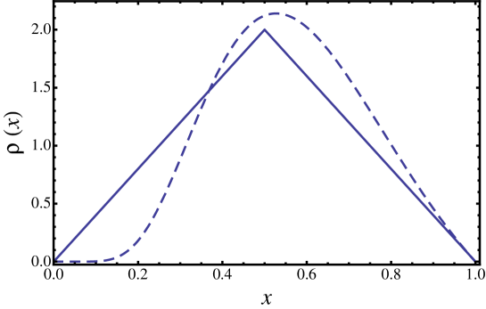
Figure 1: Probability density function of (9) (solid line) and its limiting function (dashed line).

The cumulative distribution function determined by $\rho$ is

$$\mu(x)=\begin{cases}2x^{2},&x\leq 1/2,\\ 1-2(1-x)^{2},&x>1/2,\end{cases}$$ (9)

that converges under the action of the RG transformation for $\alpha=2$ to the cumulative distribution function

$$M(x)={\rm e}^{-2(-\log x)^{2}}.$$

If we perform the expansion in (8) we obtain

$$\mu(x)=M(x)(1+2(-\log x)^{3}-\frac{19}{6}(-\log x)^{4}+\frac{9}{2}(-\log x)^{5}+\cdots).$$

The most relevant (or rather the least irrelevant) eigenvalue in the expansion is $\nu_{3}=n^{-1/2}$ and it determines the behavior with $n$ of the amplitude of the finite-size corrections. In order to quantify the corrections when the number of random variables is $n$, we use the $L^{1}$ norm for the difference of the probability densities. This norm is also called total variation metric in the context of probability theory (see HaanRes and references therein). We expand

$$\Delta:=\int_{0}^{1}|\rho_{n}(x)-M^{\prime}(x)|\hbox{d}x=c_{1/2}n^{-1/2}+c_{1}n^{-1}+c_{3/2}n^{-3/2}+\cdots$$ (10)

where $\rho_{n}=T_{s}\rho$ with $n={\rm e}^{s}$. The first coefficient is given by

$$c_{1/2}=2\int_{0}^{1}\left|\frac{\rm d}{{\rm d}x}[M(x)\log(x)^{3}]\right|\ \hbox{d}x=\frac{3}{2}\sqrt{3}{\rm e}^{-3/2},$$

and, similarly, one can compute the others to obtain

$$c_{1}=-\frac{15}{8}{\rm e}^{-3/2},\qquad c_{3/2}=\frac{9}{32}\sqrt{3}{\rm e}^{-3/2},\cdots$$

In Fig. 2 we have plotted the finite-size corrections to the distribution of the maxima obtained numerically scaled with $\sqrt{n}$, for different values of the size of the system $n$. We observe a very good agreement with the theoretical predictions in (10).

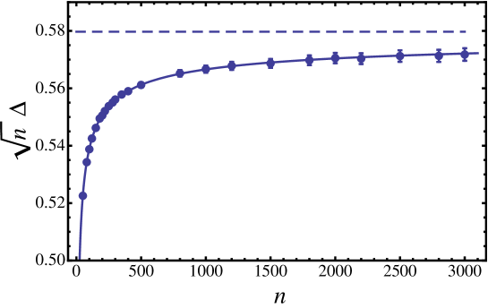
Figure 2: Finite size corrections rescaled with $\sqrt{n}$ as a function of the size of the system $n$. Dots represent the values obtained in the numerical experiment, with error bars corresponding to two standard deviations, and the solid line is the theoretical prediction for $\sqrt{n}\Delta$ up to the $n^{-1}$ term.

The second prediction that we test numerically is the shape of the corrections. In this case we take a fixed (and large) value for $n$ and we plot the rescaled difference between the limiting distribution and the one obtained numerically for the maxima of $n$ random variables distributed according to $\rho$. The finite-size corrections $\delta(x):=(\rho_{n}(x)-M^{\prime}(x))$ can be expanded as

$$\delta(x)=\delta_{1/2}(x)n^{-1/2}+\delta_{1}(x)n^{-1}+\cdots,$$

with the first coefficients given by

$$\delta_{1/2}(x) =-2\frac{\rm d}{{\rm d}x}\big{[}M(x)\log(x)^{3}\big{]},$$ (11)

$$\delta_{1}(x) =\frac{\rm d}{{\rm d}x}\big{[}M(x)\log(x)^{4}(\frac{19}{6}-2\log(x)^{2})\big{]}.$$ (12)

In Fig. 3 the dots represent the points obtained with the numerical experiment for $\sqrt{n}\delta(x)$ corresponding to $n=3000$. The error bars, a little larger than the size of the dots, represent the statistical uncertainty due to the limited size of the sample. The dashed line is $\delta_{1/2}(x)$ as defined in (11) while the solid line includes the next correction $\delta_{1/2}(x)+\delta_{1}(x)n^{-1/2}$. We see an excellent agreement between the theoretical prediction and the numerical experiment, especially when the subleading correction is included.

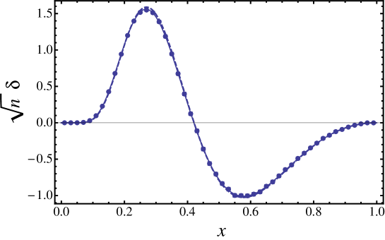
Figure 3: Shape corrections for $n=3000$. Dots represent the outcome of the numerical experiment. The error bars, representing two standard deviations, are of the order of the dot size in the plot. The dashed line is the leading term of the correction $\delta_{1/2}(x)$ while the solid line includes the next subleading term $\delta_{1/2}(x)+\delta_{1}(x)n^{-1/2}$.

The second example has a probability density

$$\rho(x)=|2-4x|,$$

and a cumulative distribution function

$$\mu(x)=\begin{cases}2x(1-x),&x\leq 1/2,\\ 1-2x(1-x),&x>1/2.\end{cases}$$

It converges under the action of the RG with $\alpha=1$ to $M(x)=x^{2}$. The limiting probability density is $M^{\prime}(x)=2x$. We can expand again,

$$\mu(x)=M(x)(1+(-\log x)^{2}+(-\log x)^{3}+\frac{7}{12}(-\log x)^{4}+\cdots),$$

and we find that the most relevant perturbation has an eigenvalue $\nu_{2}=n^{-1}$, which determines the leading behavior with $n$ of the amplitude of the finite-size corrections. If we also keep the first subleading terms we obtain

$$\Delta=\int_{0}^{1}|\rho_{n}(x)-M^{\prime}(x)|\hbox{d}x=c_{1}n^{-1}+c_{2}n^{-2}+c_{3}n^{-3}+\cdots$$ (13)

with

$$c_{1}=2{\rm e}^{-2},\quad c_{2}=3{\rm e}^{-2},\quad c_{3}=\frac{5}{2}{\rm e}^{-2}.$$

In Fig. 4 we check the validity of this expansion. We see that within the statistical errors, due to the limited size of the sample, the finite-size corrections agree with the theoretical predictions.

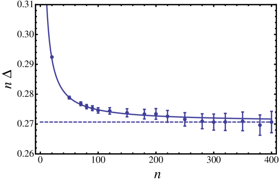
Figure 4: Finite size corrections in the second example scaled with $n$. In the $x$ axis we represent the size of the system, $n$. Dots are the values obtained from the numerical experiment and the solid line is the theoretical prediction (13) for $n\Delta$ up to the $n^{-2}$ term.

The shape of the corrections in this case is

$$\delta(x)=\delta_{1}(x)n^{-1}+\delta_{2}(x)n^{-2}+\cdots$$ (14)

with the different contributions given by

$$\delta_{1}(x) =2x\log x(1-\log x),$$ (15)

$$\delta_{2}(x) =x\log(x)^{2}(\log(x)^{2}-3).$$ (16)

In Fig. 5 we show the numerical value for the shape correction and compare it with the analytical prediction in (14). We can see again a remarkable agreement between the numerical experiment and the theoretical prediction.

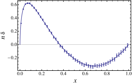
Figure 5: Shape corrections for the second example. Here $n=300$. Dots represent the outcome of the numerical experiment. The error bars stand for two standard errors. The dashed line is the leading term of the correction, $\delta_{1}(x)$, while the solid line includes the next subleading term, $\delta_{1}(x)+\delta_{2}(x)n^{-1}$. The dashed line almost coincides with the solid line; only near the maximum the small difference can be appreciated.

In the previous examples we have tested the accuracy of the finite size analysis carried out in Section IV. The size of the system and the sample have been chosen so that the computational time is reasonable and the errors are sufficiently small not to spoil any predictive power. Within this range we have to go beyond first order corrections (represented by the dashed line in Figs. 3 and 5) to give a precise description of the experimental results. The number of terms needed depends, of course, on the concrete details of the problem and the required accuracy.

VI Conclusions

By employing Renormalization Group techniques we have studied the limit distribution of the appropriately rescaled maximum value of a sequence of $n$ independent, identically distributed random variables when $n\to\infty$. Obviously, the rescaling is needed for obtaining non-trivial limits. Most of the literature on Extreme Value Theory is devoted to the study of these limits under affine rescalings, perhaps by analogy to the treatment of the problem of stable distributions. However, when computing limits of sequences of maxima of independent, identically distributed random variables, it seems natural to impose that the rescaling preserves the support of the original random variable, a condition that the affine rescaling does not meet, in general.

We have recast the problem of finding such limit distributions into the language of the Renormalization Group, explained how the condition of support preservation naturally arises, and what its implications are. The main contribution of this paper is showing that in this framework linear and non-linear rescalings are treated on an equal footing, and which one should be employed follows precisely from support preservation. In our formulation the limit distributions are fixed points of the Renormalization Group transformation. After the identification and discussion of the fixed points we have worked out the differential of the transformation around them, with emphasis on those associated to non-linear rescalings. This helps understand the domains of attraction and the corrections due to large but finite $n$, the so-called finite-size corrections.

An interesting technical aspect of the approach herein adopted is the concrete form of the definition of the Renormalization Group transformation. We define it as an uniparametric group of transformations that is fixed once for all, differing from other works in this line where the transformation can be adapted at every step. This fact has some consequences, especially concerning the domain of attraction of the fixed points. Indeed, within our approach the determination of the domain of attraction is simpler. One may wonder whether it is possible to modify the classical results on the domains of attraction when we restrict to transformations that preserve the support of the original random variable.

Finally, we would like to mention the fact that our RG fixed points are trivial in the sense that they correspond to EV for independent random variables. It would be interesting to study how these results (rescaling and fixed points) are to be modified when considering a family of correlated random variables.

Acknowledgements: I. C. acknowledges the hospitality of the Department of Theoretical Physics at the University of Zaragoza, where part of this work has been done. Research partially supported by grants 2009-E24/2, DGIID-DGA and FPA2009-09638, ENE2009-07247, Ministerio de Ciencia e Innovación (Spain).

References

- (1) L. de Haan and A. Ferreira, Extreme Value Theory: An Introduction (Springer, 2006).
- (2) R. W. Katz, M. B. Parlange, and P. Naveau, Adv. Water Resour. 25, 1287 (2002).
- (3) H. v. Storch and F. W. Zwiers, Statistical Analysis in Climate Research (Cambridge University Press, Cambridge, 2002).
- (4) B. Gutenberg and C. F. Richter, Bull. Seismol. Soc. Am. 34, 185 (1944).
- (5) J.-P. Bouchaud and M. Mézard, J. Phys. A 30, 7997 (1997).
- (6) P. Embrecht, C. Klüppelberg, and T. Mikosch, Modelling Extremal Events for Insurance and Finance (Springer, Berlin, 1997).
- (7) W. Weibull, J. Appl. Mech.-Trans. ASME 18, 293 (1951).
- (8) G. Jona–Lasinio, Nuovo Cimento 26, 98 (1975).
- (9) I. Calvo, J. C. Cuchí, J. G. Esteve and F. Falceto, J. Stat. Phys. 141, 409 (2010).
- (10) G. Gyorgyi, N. R. Moloney, K. Ozogany and Z. Racz, Phys. Rev. Lett. 100, 210601 (2008).
- (11) G. Gyorgyi, N. R Moloney, K. Ozogany, Z. Racz and M. Droz, Phys. Rev. E 81, 041135 (2010).
- (12) E. Bertin and G. Gyorgyi, J. Stat. Mech., P08022 (2010).
- (13) M. Fréchet, Ann Soc. Polonaise Math. 6, 93 (1927).
- (14) M.R. Fisher and L.H.C. Tippet, Proc. Cambridge Philos. Soc. 24, 180 (1928).
- (15) B. V. Gnedenko, Ann. Math 44, 423 (1943).
- (16) R.L. Smith, Breakthroughs in statistics, (S. Kotz and N. L. Johnson eds.) Springer-Verlag, (1993).
- (17) E. Pancheva, ProbStat Forum 3, 11 (2010).
- (18) E. Pancheva, Lecture Notes in Math., 1155, 284 (1984).
- (19) N.R. Mohan and S. Ravi, Theory Probab. Appl. 37, 632 (1991).
- (20) S. M. Popov, G. Lerosey, R. Carminati, M. Fink, A. C. Boccara and S. Gigan, Phys. Rev. Lett. 104, 100601 (2010).
- (21) M.S. Oey and C.J. Clarke, Astrophysical J. 620, L43-46 (2005).
- (22) L. de Haan and S. Resnick, The Annals of Probability 24, 97 (1996).