Replicated Échelle Diagrams in Asteroseismology: A Tool for Studying Mixed Modes and Avoided Crossings

Abstract

In oscillating stars, mixed modes have p-mode character in the envelope and g-mode character in the core. They are observed in subgiants and red giants, in which the large density gradient outside the core effectively divides the star into two coupled cavities. This leads to the phenomenon of mode bumping, in which mode frequencies are shifted from their regular spacing as they undergo avoided crossings. This short contribution introduces a new diagram that involves extending the traditional échelle diagram by replication. This new diagram should prove a useful way of displaying mixed modes and helping to identify missing modes that may lie below the detection threshold.

1 Mixed modes and avoided crossings

Asteroseismology involves using the oscillation frequencies of stars to extract information about their parameters and internal structures. For solar-type main-sequence stars, the observed oscillations are pure p modes (acoustic waves, for which the restoring force arises from the pressure gradient). These are regularly spaced in frequency, closely following the so-called asymptotic relation (Tassoul 1980; Gough 1986). However, the oscillations of post-main-sequence stars show departures from this regularity that are due to the presence of mixed modes.

Mixed modes have p-mode character in the stellar envelope and g-mode character in the core (g modes are gravity modes, for which the restoring force is buoyancy). Mixed modes occur in evolved stars (subgiants and red giants), in which the large density gradient outside the core effectively divides the star into two coupled cavities. This leads to the phenomenon of mode bumping, in which mode frequencies are shifted from their regular spacing (for more details, see Scuflaire 1974; Osaki 1975; Aizenman et al. 1977; Dziembowski & Pamyatnykh 1991; Christensen-Dalsgaard 2004; Miglio et al. 2008; Aerts et al. 2010; Deheuvels & Michel 2010a; Deheuvels & Michel 2011; Bedding 2011).

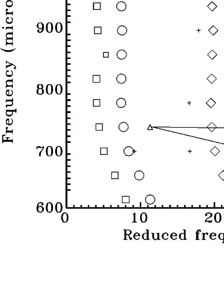
Figure 1 shows theoretical oscillations frequencies for the subgiant star $\eta$ Boo, calculated by Christensen-Dalsgaard et al. (1995). The left panel shows the evolution with time of the model frequencies for modes with $l=0$ (dashed lines) and $l=1$ (solid lines). The $l=0$ frequencies decrease slowly with time as the star expands. At a given moment in time, such as that marked by the vertical line, the radial modes are regularly spaced in frequency, with a large separation of $\mbox{$\Delta\nu$}\approx 40\,\mbox{$\mu$Hz}$. However, the behaviour is rather different for the $l=1$ modes (solid lines). They undergo a series of avoided crossings as a function of time (Osaki 1975; Aizenman et al. 1977), during which an $l=1$ mode is bumped upwards by the mode below, and in turn it bumps the mode above. The effect is to disturb the regular spacing of the $l=1$ modes in the vicinity of each avoided crossing, squeezing the modes together. As discussed by Bedding (2011), the frequencies of the avoided crossings correspond to g modes trapped in the core of the star (referred to as $\gamma$ modes, following Aizenman et al. 1977).

The right panel of Fig. 1 shows the frequencies in échelle format (Grec et al. 1983) for the single model that is marked in the left panel by the vertical line. The bumping from regularity of the $l=1$ modes (triangles) is obvious. It is important to note there this is one extra $l=1$ mode at each avoided crossing.

Figure 1.: Left: Evolution of oscillation frequencies in models of a subgiant star of mass $1.60\mbox{$M_{\odot}$}$ and $Z=0.03$ (representing $\eta$ Boo). The dashed lines correspond to modes of degree $l=0$, and the solid lines to $l=1$. The vertical solid line indicates the location of the model whose frequencies are illustrated in the right panel. Right: Échelle diagram using a frequency separation of $\Delta\nu=40.3\mbox{$\mu$Hz}$ and a zero-point frequency of $\nu_{0}=735\mbox{$\mu$Hz}$. Circles are used for modes with $l=0$, triangles for $l=1$, squares for $l=2$ and diamonds for $l=3$. The size of the symbols indicates the relative amplitude of the modes, estimated from the mode inertia, with crosses used for modes whose symbols would otherwise be too small. Figures adapted from Christensen-Dalsgaard et al. (1995).

Bumping of $l=1$ modes has been observed and modelled in several subgiant stars:

• $\eta$ Boo (Kjeldsen et al. 1995; Christensen-Dalsgaard et al. 1995; Guenther & Demarque 1996; Di Mauro et al. 2003a; Kjeldsen et al. 2003; Guenther 2004; Carrier et al. 2005),

• $\beta$ Hyi (Di Mauro et al. 2003b; Fernandes & Monteiro 2003; Bedding et al. 2007; Brandão et al. 2011),

• the CoRoT target HD 49385 (Deheuvels et al. 2010; Deheuvels & Michel 2010a, b; Deheuvels & Michel 2011)

• the Kepler target KIC 11026764 (‘Gemma’; Chaplin et al. 2010; Metcalfe et al. 2010),

• the Kepler target KIC 11234888 (‘Tigger’; Mathur et al. 2011),

• the Kepler target KIC 11395018 (‘Boogie’; Mathur et al. 2011),

• the Kepler target KIC 10273246 (‘Mulder’; Campante et al. 2011) and

• the Kepler target KIC 10920273 (‘Scully’; Campante et al. 2011).

For Procyon, which is close to the end of the main sequence, Bedding et al. (2010) suggested a possible $l=1$ mixed mode at low frequency, based on the narrowness of the peak in the power spectrum. Note that mixed modes are expected to have longer lifetimes (smaller linewidths) than pure p modes because they have larger mode inertias (e.g., Christensen-Dalsgaard 2004).

The aim of this short contribution is to introduce a way of extending the échelle diagram by replication, which may be useful in the study of mixed modes. Before doing so, we note that there are two ways to make an échelle diagram. One is to keep the orders horizontal — the échelle diagram in Fig. 1 uses this convention. Alternatively, one can plot $\nu$ versus ($\nu\bmod\mbox{$\Delta\nu$}$), in which case each order slopes upwards. An example of this is discussed below (Fig. 4).

2 The Replicated Échelle Diagram

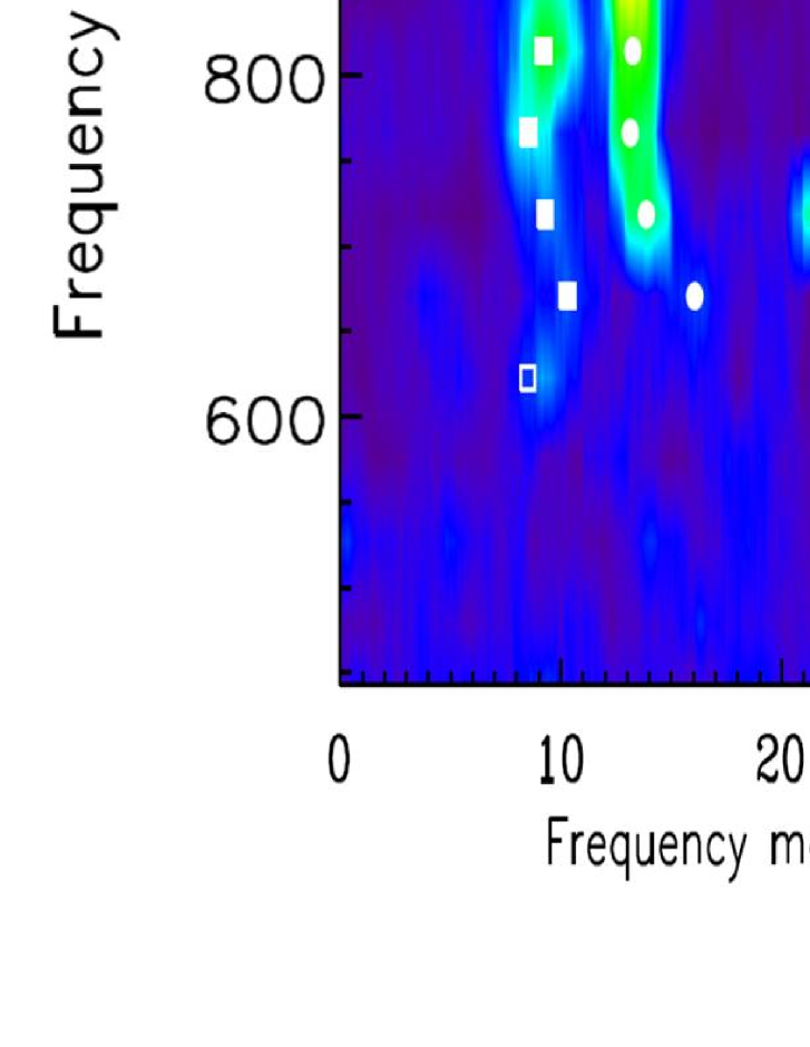
Figure 2 was made by replicating the échelle diagram shown in Fig. 1. For reasons that will become clear, each copy is displaced downwards by one order, that is, by $\Delta\nu$ in frequency. The thick red lines connect the $l=1$ modes and traces a smooth curve, without the “wrapping” that occurs in a standard échelle diagram.

Figure 2.: Replicated échelle diagram of the model of $\eta$ Boo that is shown in the right panel of Fig. 1. The thick red lines connect the $l=1$ modes.

Figure 3.: Replicated échelle diagram based on observations of KIC 11395018 (‘Boogie’) by Mathur et al. (2011). The red lines connect the $l=1$ modes.

This type of figure allows us to see more clearly when modes are missing. For example, Fig. 3 shows the replicated échelle diagram for the Kepler target KIC 11395018 (‘Boogie’), based on the power spectrum observed by Mathur et al. (2011). As mentioned above, we expect to see one extra $l=1$ mode at each avoided crossing. Because of the way the replicated échelle diagram is constructed, with an offset of one order between each panel, we expect one $l=1$ mode in every horizontal row. In Fig. 3 we see there is a missing $l=1$ mode near the top, which must lie between the $l=0$ and $l=2$ modes (see the middle panel) and could be detected when more data become available.

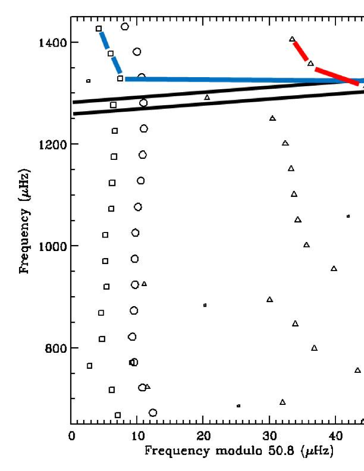
Another example is shown in Fig. 4, using model frequencies calculated by Metcalfe et al. (2010) for the Kepler target KIC 11026764 (‘Gemma’). This time we show two curves, corresponding to $l=1$ modes (red) and $l=2$ modes (blue). Note that each curve moves to a new panel at each avoided crossing, and we see that the avoided crossings for $l=2$ are more closely spaced than for $l=1$. This occurs because the frequencies of the avoided crossings correspond to g modes trapped in the core of the star (the so-called $\gamma$ modes — see above) and we know from asymptotic theory (Tassoul 1980) that their period spacing is inversely proportional to $\sqrt{l(l+1)}$ (see Eq. 3.236 of Aerts et al. 2010, where the quantity $L=\sqrt{l(l+1)}$ is defined after Eq. 3.197).

Figure 4.: Replicated échelle diagram based on a model of KIC 11026764 (‘Gemma’; Model AA by Metcalfe et al. 2010). Red and blue lines connect $l=1$ and $l=2$ modes, respectively. The black lines mark one of the upward-sloping orders.

The shape of each curve contains information about the strength of the coupling between the p- and g-mode cavities. As discussed by Deheuvels & Michel (2010a); Deheuvels & Michel (2011), the coupling strength determines the details of the mode bumping, including the number of modes that are affected. In the replicated échelle diagrams, the coupling strength could be measured at each avoided crossing from the gradient of the inflection point. We can see from Fig. 4 that the coupling for the $l=2$ modes is much weaker than for $l=1$ modes, as discussed by Christensen-Dalsgaard (2004).

The replication in Fig. 4 does not include a vertical offset between panels. This is because this échelle diagram was made with the sloping orders (one of which is enclosed by a pair of black lines), whereas those in Figs. 2 and 3 were plotted with horizontal orders (see Sec. 1). In both types of diagram, the construction method ensures that the curve connects modes such that there is exactly one in each ‘row’ (whether the rows be horizontal or sloping). Put another way, the modes occur along the curve at the points where it intersects with each row. One can envisage fitting an analytical function to this curve; the $\arctan$ function would appear to be a good choice.

Acknowledgments

Many thanks to our Japanese hosts for a fantastic workshop under very difficult conditions. I also thank Othman Benomar, Jørgen Christensen-Dalsgaard, Hans Kjeldsen, Dennis Stello and Tim White for helpful discussions.

References

- Aerts et al. (2010) Aerts, C., Christensen-Dalsgaard, J., & Kurtz, D. W. 2010, Asteroseismology (Springer: Heidelberg)
- Aizenman et al. (1977) Aizenman, M., Smeyers, P., & Weigert, A. 1977, A&A, 58, 41
- Bedding (2011) Bedding, T. R. 2011, in Asteroseismology, edited by P. L. Pallé (Cambridge University Press), vol. XXII of Canary Islands Winter School of Astrophysics. In press (arXiv:1107.1723)
- Bedding et al. (2001) Bedding, T. R., Butler, R. P., Kjeldsen, H., et al. 2001, ApJ, 549, L105
- Bedding et al. (2007) Bedding, T. R., Kjeldsen, H., Arentoft, T., et al. 2007, ApJ, 663, 1315
- Bedding et al. (2010) Bedding, T. R., Kjeldsen, H., Campante, T. L., et al. 2010, ApJ, 713, 935
- Brandão et al. (2011) Brandão, I. M., Doğan, G., Christensen-Dalsgaard, J., et al. 2011, A&A, 527, A37
- Campante et al. (2011) Campante, T. L., Handberg, R., Mathur, S., et al. 2011, A&A. Submitted
- Carrier et al. (2001) Carrier, F., Bouchy, F., Kienzle, F., et al. 2001, A&A, 378, 142
- Carrier et al. (2005) Carrier, F., Eggenberger, P., & Bouchy, F. 2005, A&A, 434, 1085
- Chaplin et al. (2010) Chaplin, W. J., Appourchaux, T., Elsworth, Y., et al. 2010, ApJ, 713, L169
- Christensen-Dalsgaard (2004) Christensen-Dalsgaard, J. 2004, Sol. Phys., 220, 137
- Christensen-Dalsgaard et al. (1995) Christensen-Dalsgaard, J., Bedding, T. R., & Kjeldsen, H. 1995, ApJ, 443, L29
- Deheuvels et al. (2010) Deheuvels, S., Bruntt, H., Michel, E., et al. 2010, A&A, 515, A87
- Deheuvels & Michel (2010a) Deheuvels, S. & Michel, E. 2010a, Ap&SS, 328, 259
- Deheuvels & Michel (2010b) — 2010b, Astron. Nachr., 331, 929
- Deheuvels & Michel (2011) — 2011, A&A. In press (arXiv:1109.1191)
- Di Mauro et al. (2003a) Di Mauro, M. P., Christensen-Dalsgaard, J., Kjeldsen, H., Bedding, T. R., & Paternò, L. 2003a, A&A, 404, 341
- Di Mauro et al. (2003b) Di Mauro, M. P., Christensen-Dalsgaard, J., & Paternò, L. 2003b, Ap&SS, 284, 229
- Dziembowski & Pamyatnykh (1991) Dziembowski, W. A. & Pamyatnykh, A. A. 1991, A&A, 248, L11
- Fernandes & Monteiro (2003) Fernandes, J. & Monteiro, M. J. P. F. G. 2003, A&A, 399, 243
- Gough (1986) Gough, D. O. 1986, in Hydrodynamic and Magnetodynamic Problems in the Sun and Stars, edited by Y. Osaki (Tokyo: Uni. of Tokyo Press), 117
- Grec et al. (1983) Grec, G., Fossat, E., & Pomerantz, M. A. 1983, Sol. Phys., 82, 55
- Guenther (2004) Guenther, D. B. 2004, ApJ, 612, 454
- Guenther & Demarque (1996) Guenther, D. B. & Demarque, P. 1996, ApJ, 456, 798
- Kjeldsen et al. (2003) Kjeldsen, H., Bedding, T. R., Baldry, I. K., et al. 2003, AJ, 126, 1483
- Kjeldsen et al. (1995) Kjeldsen, H., Bedding, T. R., Viskum, M., & Frandsen, S. 1995, AJ, 109, 1313
- Mathur et al. (2011) Mathur, S., Handberg, R., Campante, T. L., et al. 2011, ApJ, 733, 95
- Metcalfe et al. (2010) Metcalfe, T. S., Monteiro, M. J. P. F. G., Thompson, M. J., et al. 2010, ApJ, 723, 1583
- Miglio et al. (2008) Miglio, A., Montalbán, J., Eggenberger, P., & Noels, A. 2008, Astronomische Nachrichten, 329, 529
- Osaki (1975) Osaki, J. 1975, PASJ, 27, 237
- Scuflaire (1974) Scuflaire, R. 1974, A&A, 36, 107
- Tassoul (1980) Tassoul, M. 1980, ApJS, 43, 469