Codimension-two homoclinic bifurcations underlying spike adding in the Hindmarsh-Rose burster

Abstract

The well-studied Hindmarsh-Rose model of neural action potential is revisited from the point of view of global bifurcation analysis. This slow-fast system of three paremeterised differential equations is arguably the simplest reduction of Hodgkin-Huxley models capable of exhibiting all qualitatively important distinct kinds of spiking and bursting behaviour. First, keeping the singular perturbation parameter fixed, a comprehensive two-parameter bifurcation diagram is computed by brute force. Of particular concern is the parameter regime where lobe-shaped regions of irregular bursting undergo a transition to stripe-shaped regions of periodic bursting. The boundary of each stripe represents a fold bifurcation that causes a smooth spike-adding transition where the number of spikes in each burst is increased by one. Next, numerical continuation studies reveal that the global structure is organised by various curves of homoclinic bifurcations.

In particular the lobe to stripe transition is organised by a sequence of codimension-two orbit- and inclination-flip points that occur along each homoclinic branch. Each branch undergoes a sharp turning point and hence approximately has a double-cover of the same curve in parameter space. The sharp turn is explained in terms of the interaction between a two-dimensional unstable manifold and a one-dimensional slow manifold in the singular limit. Finally, a new local analysis is undertaken using approximate Poincaré maps to show that the turning point on each homoclinic branch in turn induces an inclination flip that gives birth to the fold curve that organises the spike-adding transition. Implications of this mechanism for explaining spike-adding behaviour in other excitable systems are discussed.

1 Introduction

The Hindmarsh-Rose (HR) model [23] is one of the most widely studied parameterised three-dimensional systems of ordinary differential equations (ODEs) that arises as a reduction of the conductance-based Hodgkin-Huxley model for neural spiking [24]. Its success comes from both its simplicity — just three ODEs with polynomial nonlinearity, and only a few key parameters — and its ability to qualitatively capture the three main dynamical behaviours displayed by real neurons, namely quiescence, tonic spiking and bursting (see Fig. 1). Moreover, transitions between these behaviours can be easily described in terms of the bio-physically motivated parameters. Even reduced-order models like the HR equations can have direct physiological meaning and so can be used to match or indeed predict detailed in vivo recordings; for instance, in [10] the authors use the HR model – after appropriately rescaling the state variable $x$, the parameter $I$ and time – to fit the activity of both pyramidal cells and neocortical interneurons. Nevertheless, a key argument for their use is that they can point to generic understanding of which kinds of interventions or perturbations are likely to lead to certain kinds of transition. These understandings can then be used to help guide parameter searches for more in-depth computational models which can only be investigated by direct numerical simulation (DNS). In turn, these simulations can help guide experimental or clinical control strategies or protocols.

Many papers have investigated the bifurcations that occur in the HR model upon variation of one or more of its parameters; see [4, 18, 19, 27, 28, 45, 47, 48, 49, 50]. These studies have typically focussed on particular transitions: from periodic to irregular (chaotic) spiking-bursting dynamics, from tonic spiking to bursting and on the two possible kinds of bursting (square-wave and pseudo-plateau). For perhaps the most comprehensive bifurcation analysis to date the reader is referred to the work of Shilnikov & Kolomiets [45].

In this paper we shall be concerned with understanding the complete bifurcation scenario that underlies the smooth transition from tonic spiking to bursting, paying particular attention to an observed sequence of spike-adding transitions. This form of period-adding behaviour would cause a variation of the average number of spikes within a burst, which behaviour is believed to have important physiological implications [39]. The key point of the paper is to show that codimension-one homoclinic bifurcations and their degeneracies are crucial to understanding how such transitions are organised in parameter space. The methodology we shall adopt will be a combination of brute-force methods (augmenting the preliminary results in [47]), slow-fast arguments, numerical continuation (using AUTO07P [14]), and geometric analysis using approximate Poincaré maps.

Brute-force methods involve classification of stable asymptotic behaviour computed using DNS over a wide range of parameter values. When trying to understand the mechanisms behind observed transitions in stable behaviour though, such methods can only describe bifurcation scenarios roughly. In particular, they often fail to uncover coexisting attractors, and they do not compute the unstable invariant sets that are often crucial in isolating and analysing both local and global bifurcations.

From a more analytic point of view, the HR model can be decomposed into a reduced two-dimensional “fast” ODE-system with an additional slow variable. Such slow-fast arguments, see [5, 17, 29, 41, 45], can provide much generic information about the original model and tend to work best close to the singular limit of infinite time-scale separation. However, most physical systems operate away from the singular limit, and the mutual interactions between slow and fast dynamics are typically very subtle and give rise to further bifurcations in the complete system that occur “beyond all orders” in the singular limit.

Numerical continuation analysis [31] is typically quite robust and through its use of boundary-value problems to solve for recurrent trajectories does not suffer from the same problems as DNS in the singular limit. Nevertheless, as we shall see, problems can still arise in the presence of “canard-like” phenomena [12, 20]. In this case, a mix of numerical results and geometrical analysis can prove pivotal.

The rest of this paper is organised as follows. The next section introduces the Hindmarsh-Rose model and its dynamics, in particular highlighting its slow-fast structure. Section 3 then presents numerical bifurcation analysis computed both by brute force and through numerical continuation. Particular attention is focussed on an infinite family of bifurcation curves of homoclinic orbits that connect an equilibrium on the unstable part of the critical manifold to itself. Various codimension-two homoclinic bifurcation points are detected and local bifurcation curves arising from them are computed. It is found that the key fold bifurcations underlying spike-adding transitions originate from sharp turning point along the homoclinic bifurcation curves, caused by the interaction between a 1D slow manifold and a 2D unstable manifold of an equilibrium point. Owing to the sharpness of the folding of the unstable manifold, numerical continuation is found to be inconclusive. Section 4 therefore presents a new geometric analysis of such a situation and shows that there has to be an additional codimension-two homoclinic bifurcation of inclination flip type very close to this point of interaction. Finally section 5 draws conclusions, suggests avenues for further work, and points to some wider implications of the results.

2 The Hindmarsh-Rose model

Typical spiking neurons occurring across biology can undergo a variety of distinct dynamical behaviours, according to the values of bio-physical parameters. See Fig. 1 for outputs from a biologically relevant neuron model. Among the most important behaviours, one may find [29]:

• quiescence, which occurs when the input to the neuron is below a certain threshold and the output does not include any action potential firing events (or spikes);

• spiking, in which the output is made up of a regular series of spikes;

• bursting, where the output consists of groups of two or more spikes separated by periods of inactivity;

• irregular spiking: the output is made up of an aperiodic series of spikes.

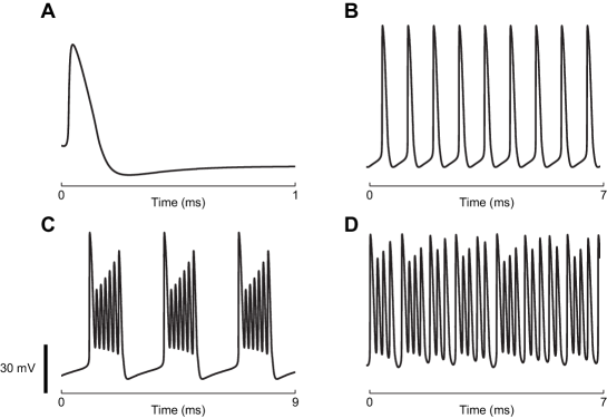
Figure 1: Typical membrane potentials computed using a model of a leech heart interneuron showing, under varying input parameters, (A) quiescence, (B) spiking, (C) bursting and (D) irregular spiking. The model is as in [43], with parameters $C=0.5$, $E_{K}=-0.07$, $E_{Na}=0.045$, $g_{Na}=200$, $g_{1}=8$, $E_{1}=-0.046$, $\tau_{Na}=0.0405022$, $V_{K2}^{shift}=-0.0145$ and $g_{K2}=30$ and: (A) $I_{app}=-0.02$, $\tau_{K2}=0.25$; (B) $I_{app}=0$, $\tau_{K2}=0.2$; (C) $I_{app}=0$, $\tau_{K2}=1$; (D), $I_{app}=0.07$, $\tau_{K2}=0.35$.

Previous studies have shown that the HR model is able to reproduce all these dynamical behaviours [4, 18, 19, 27, 28, 45, 47, 48, 49, 50]. Moreover, in these references bifurcation analysis has been carried out in one or two parameters, unfolding cascades of smooth transitions between stable bursting solutions and continuous spiking regimes, both regular (periodic) and irregular (chaotic). See Fig. 4 below for a recapitulation of some of these results in a two-parameter bifurcation diagram.

2.1 The governing equations

The phenomenological neuron model proposed by Hindmarsh and Rose (HR) [22, 23] is a single-compartment model that is computationally simple yet is capable of mimicking the rich variety of firing pattern behaviours exhibited by real biological neurons [21]. It can be described by the following set of ODEs:

$$\left\{\begin{array}[]{@{}r@{}c@{}l}\dot{x}&=&y-x^{3}+bx^{2}+I-z\\[5.0pt] \dot{y}&=&1-5x^{2}-y\\[5.0pt] \dot{z}&=&\mu\left(s\left(x-x_{rest}\right)-z\right)\end{array}\right.$$ (1)

The model is dimensionless and the variables have only phenomenological interpretations. The variables $x$ and $y$ represent the fast charging dynamics (voltage and current respectively) associated with a single neuron whereas $z$ is a slow variable mirroring the action of slow ionic channels. Hence, (1) is a slow-fast system with two fast and one slow variable. Its fast nullcline $M_{eq}:=\{(x,y,z)\in\mathbb{R}^{3};\;z=y-x^{3}+bx^{2}+I,\;y=1-5x^{2}\}$ is the so-called critical manifold of the system. The critical manifold $M_{eq}$ is a manifold of equilibria for the limiting problem obtained by setting $\mu=0$ in (1), and plays a crucial role in the non-trivial dynamics of the full system; see section 2.2 below. The roles played by the system parameters can be described as follows. The parameter $I$ mimics the membrane input current for biological neurons, whereas $b$ is an excitability parameter that allows one to switch between bursting and spiking behaviours and to control the spiking frequency. The variable $\mu$ controls the time scale of the slow variable $z$, that is, the efficiency of the slow channels in exchanging ions. In the presence of spiking behaviour, it affects the inter-spike interval, whereas in the case of bursting it affects the number of spikes per burst. The phenomenological parameter $s$ governs the degree of adaptation in the neuron. A value of $s$ around unity causes spiking behaviour with no spike-frequency accommodation nor subthreshold adaptation, whereas values around $s=4$ (the value we shall use in this paper) allow strong accommodation and subthreshold overshoot, and can even allow oscillations. The parameter $x_{rest}$ sets the resting potential of the system and is usually set to $-1.6$ in the dimensionless units in which 1 is written.

In what follows, unless otherwise stated we shall consider 1 at parameter values

$$s=4,\qquad x_{rest}=-1.6,\qquad\mu=0.01$$ (2)

and allow $I$ and $b$ to be bifurcation parameters.

2.2 Spike adding and slow-fast analysis

A key feature displayed by many neuronal models is the so-called spike adding mechanism: this means that it is possible, by changing one parameter, to smoothly change the behaviour of the system from spiking to bursting with increasing number of spikes per bursts, as shown in Fig. 2. In the HR model, changing the parameter $b$ allows one to observe this transition among periodic responses. To some extent, also raising the injected current $I$ leads to this spike adding, but this also typically increases frequency of the bursts. Other combinations of parameters, e.g., $\mu$ and $I$, lead to similar results [19, 40, 47].

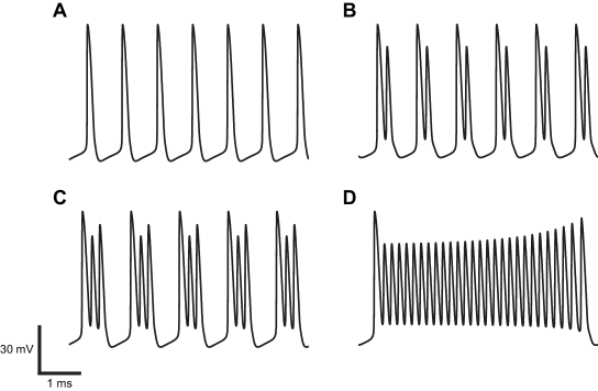
Figure 2: Examples of period adding in the same model as in Fig. 1. By varying a single parameter, periodic responses can be observed which undergo a transition from (A) isolated spikes, to (B) two spikes per burst, to (C) three spikes per burst, and so on, up to (D) 28 spikes per burst. Model and parameters as in Fig. 1 but with $I_{app}=0$ and $\tau_{K2}=0.2$, $0.3$, $0.5$ and $3.5$ for panels A to D respectively.

One of the most widely used approaches to analyse period-adding in the HR and related models is so-called slow-fast analysis [11, 20, 43, 44, 45, 48]. The technique consists of separating the model into two or more ODE subsets, corresponding to parts of the neuron that operate on different time scales, for example membrane voltage and fast currents on the one hand and slow currents and calcium dynamics on the other hand. We shall now provide an overview of such analysis in system (1). The fast subsystem is given by the equations

$$\left\{\begin{array}[]{l}\dot{x}=y-x^{3}+bx^{2}+I-z\\ \dot{y}=1-5x^{2}-y.\end{array}\right.$$ (3)

which contain only two out of the five initial parameters ($b$ and $I$), but in the limit $\mu=0$, $z$ becomes a constant parameter. Note that the critical manifold $M_{eq}$ of system (1) corresponds to the set of equilibrium points of the fast subsystem (3). To illustrate this point, Fig. 3A depicts a one-parameter bifurcation analysis of system 3 obtained by varying $z$ and keeping $b=2.6$ and $I=2$ fixed. There is a curve of equilibria (shown in green in the figure) which is stable for large $z$ and undergoes two folds $f^{1,2}$, becomes stable again before loosing stability at a supercritical Hopf bifurcation $H^{-}$. The grey vertical lines are the projections onto the $(z,x)$ plane of the stable limit cycles of system (3), which organise the bursting behaviour of the full HR model. It is interesting to note that for the particular $b$ and $I$ values chosen, at around $z=2.5$ the stable limit cycle becomes close to the unstable equilibrium that exists between $f^{1}$ and $f^{2}$. The system is therefore close to a homoclinic bifurcation, and indeed we observed the typical drop-shaped cycles which are characteristic of homoclinic trajectories.

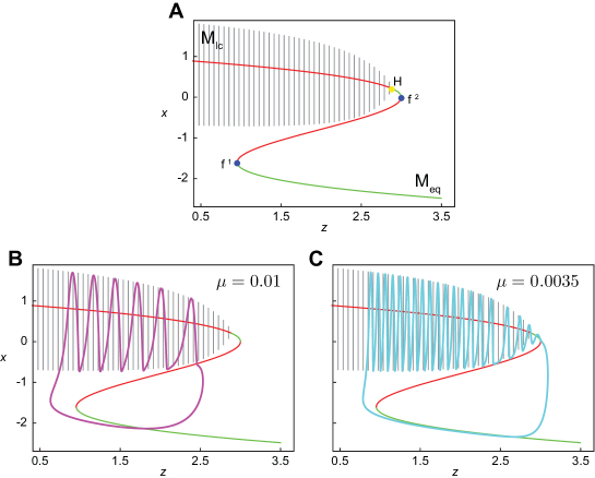
Figure 3: Slow-fast decomposition of bursting in the HR neuron model with $b=2.6$ and $I=2$. Panel A shows the bifurcation analysis of the fast subsystem obtained by varying the slow variable $z$ considered as a parameter. Panels B and C show solutions of the full HR model for different values of $\mu$: it is evident that the value of $\mu$ influences the number of turns of the solution around the manifold of limit cycles, i.e., the number of spikes per burst. See text for more details.

The results of this simple bifurcation analysis for $\mu=0$ constitute the skeleton of the solution of the full HR model (for $\mu>0$). In particular, for sufficiently small $\mu$ geometric singular perturbation theory [16] gives, away from the non-hyperbolic points — here, fold points — of the critical manifold $M_{eq}$ (as equilibria of the fast subsystem) the existence of centre-like (hence, non-unique) one-dimensional perturbed (locally invariant) manifolds $O(\mu)$-close to the manifold $M_{eq}$ of equilibria. Families of hyperbolic equilibria of the fast dynamics are referred to as normally hyperbolic invariant manifolds for the full system [30]. These perturbed manifolds are called slow (or Fenichel) manifolds. Fenichel theory [15, 16] accounts for their existence and behaviour near hyperbolic equilibrium points of the fast dynamics only; however, close to non-hyperbolic points, they can be extended by the flow and their behaviour can be understood using other analytical techniques such as geometric desingularization or blow-up [32]. Furthermore, generalised Fenichel theory [15] also accounts for the persistence of manifolds of fast motion from the singular limit $\mu=0$ to the $0<\mu\ll 1$ case. In the particular case we are investigating here, the family of limit cycles of the fast subsystem, parameterised by the (frozen) slow variable $z$, is hyperbolic and, hence, persists as a two-dimensional manifold $M_{lc}$ close to these limit cycles.

A simple explanation of bursting in the full model is that the solution repeatedly switches between $M_{eq}$ and $M_{lc}$ under the action of the slow variable $z$. This leads to periods of activity, the bursts, in which the solution evolves close to $M_{lc}$ interspersed with periods of quiescence, in which the solution moves close to $M_{eq}$. To better clarify this concept, panels B and C of Fig. 3 show the projections onto the $(z,x)$-plane of two bursting solutions of the complete system for different values of $\mu$. For $\mu=0.01$ (panel B), the number of spikes per burst is 6, whereas $\mu=0.0035$ (panel C) leads to bursts with 20 spikes (panel C). The increased number of spikes is due to the fact that, smaller $\mu$ causes slower trajectories along the $z$-direction. As a consequence, the solution stays for a longer period of time close to $M_{lc}$ and, because the fast rotation within $M_{lc}$ happens at a $\mu$-independent rate, the number of spikes per burst increases as $\mu$ decreases. Note that the fast subsystem (3) is by definition independent of $\mu$, so one can superimpose the attractor of the full system onto the bifurcation diagram of (3) for any value of $\mu$. As we shall see, depending on the values of all the other parameters, these hybrid bursting trajectories can be either periodic, quasi-periodic or chaotic. In parameter regions where periodic responses are found, the mechanism by which new spikes are added is complex and involves interaction of the bursting region with the fold $f^{1}$ of the critical manifold. The main purpose of this paper then is to provide a bifurcation theoretic explanation of period-adding process. In particular we shall seek an explanation that works for general $\mu$-values without reference to slow-fast analysis.

3 Numerical bifurcation analysis

Figure 4 shows a brute-force bifurcation diagram of the region of interest.

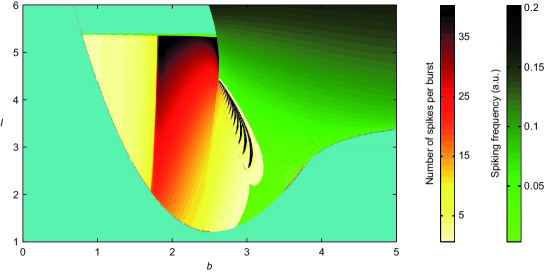
Figure 4: Brute force bifurcation diagram of the HR model 1, for the set of parameter values 2, in the $(b,I)$-plane. See text for full explanation of the colour map.

The bifurcation diagram indicates that the HR model is able to reproduce all the dynamical behaviours indicated in the previous section. In particular, the colour code is as follows:

• represents quiescence;

• is for spiking, with darker tones corresponding to a higher steady-state firing frequency;

• are used to represent regular bursting (stable periodic orbits), more specifically yellow changes to red as the number of spikes per burst increases;

• represents irregular spiking, which, from a dynamical system’s point of view, corresponds to chaotic behaviour.

See [47] for an explanation of the techniques used. One of the weaknesses of the method is that the presence of regions admitting coexisting asymptotic behaviours cannot be directly inferred from the colour map.

3.1 The regular-to-irregular bursting transition

In terms of bifurcation analysis, the area with the richest dynamics in Fig. 4 occurs in the region $b\in[2.5,3.2]$, $I\in[2,4.5]$. Here we can observe lobe-shaped regions of irregular bursting and stripe-shaped regions of regular bursting, with each successive stripe corresponding to one extra spike per period. To try to understand the mechanism by which this transition from regular to irregular bursting regions occurs, Fig. 5 shows a zoom of the parameter region in question with three different sets of bifurcation curves superimposed. These curves were computed using numerical continuation in the software AUTO-07p[14] and its extension HomCont for the localisation of codimension-two homoclinic bifurcation points.

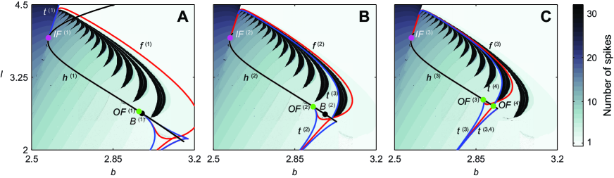
Figure 5: Numerically computed bifurcation curves showing (in panels A, B and C respectively) bifurcations associated with one, two and three bursts per period. See text for details.

In the diagram, we have adopted the following colour and labelling code for the bifurcations curves

• folds of cycles (tangent bifurcations) are labelled $t$ and coloured blue;

• period doublings (flips) are labelled $f$ and coloured red;

• homoclinic bifurcations are labelled $h$ and coloured black.

Moreover, the superscript index indicates the approximate number of spikes per period of the limit cycle (or homoclinic orbit) undergoing the bifurcation. So, for example, the label $f^{(1)}$ indicates a period doubling bifurcation curve involving a 1-spike cycle. Note that each of the flips typically represents the first in an entire period-doubling cascade. Superscripts $(n,m)$ indicate that the cycle involved in the bifurcation undergoes a transition from $n$ to $m$ spikes as is typical of bifurcations involved in the period adding mechanism. In addition we use letters to distinguish distinct bifurcations of the same kind, e.g. $h^{(2)}$ and $h^{(2a)}$ will represent different homoclinic orbits that have two spikes.

In Fig. 4 we have also identified several codimension-two homoclinic bifurcation points. Specifically purple, green and black dots indicate respectively inclination flip, orbit flip and Belyakov points. An inclination flip bifurcation represents a point along a curve of homoclinic orbits to a real saddle at which the orientability of the global stable or unstable manifold changes, see Fig. 6. For information on the complex codimension-one curves that can emanate from the codimension-two point see for example [25, 26] and references therein. In particular, there are three topologically distinct cases. An orbit flip occurs when the trajectory undergoing the homoclinic orbit flips between the two components of the (weak) stable or unstable manifold. In the case of a real saddle in three dimensions, the same three topological cases apply as for the inclination flip, again see [42, 25] and references therein. A Belyakov bifurcation [1, 2, 3] occurs when the leading eigenvalues (closest to the imaginary axis) of the saddle-point involved in the homoclinic orbit are double and undergo a transition to a complex pair. The theory predicts the presence of several families (of infinite cardinality) of bifurcation curves originating at these points and accumulating exponentially on the homoclinic curve. See [7, 33, 46] for more details of the dynamics near codimension-two homoclinic bifurcations.

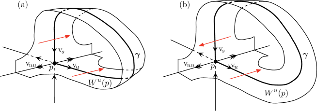
Figure 6: Schematic representation of an inclination flip bifurcation in the case (relevant to Eq. (1)) of a saddle equilibrium in a three-dimensional vector field with a two-dimensional unstable manifold. The two panels show the same homoclinic orbit before (panel (a)) and after (panel (b)) the bifurcation; note how the unstable manifold changes from orientable to non-orientable between panels (a) and (b), respectively. The notation is as described in Sec. 4 below.

As we shall see in more detail shortly, these codimension-two points, and more besides, play a key role in unfolding the regular to irregular bursting transitions.

Note that each of the three homoclinic bifurcation curves computed in Fig. 5 actually represents an approximate double cover of the same curve in parameter space, with the seeming endpoint of the curve in fact representing a sharp $U$-turn. Therefore the fine structure of the bifurcation curves is not apparent without looking at the particular shapes of the trajectories, which will be elucidated in the following subsections. The structure of the homoclinic curve $h^{(3)}$ and the associated local bifurcations of cycles depicted in panel C of Fig. 5 is similar to that relevant for all subsequent lobe-to-stripe transitions for $k>3$. Therefore the case $k=3$ will serve as an illustrative example in what follows. The cases for $k=1$ and $k=2$ (depicted in panels $A$ and $B$ respectively) are special and will be dealt with separately.

Before proceeding with a more in-depth examination of the homoclinic bifurcations, it is worth showing out how the local bifurcations of cycles that bifurcate below the homoclinic bifurcation curves organise the boundaries of the stripe-shaped periodic bursting regions. Figure 7 shows in detail the bifurcations associated with the spike-adding boundary between the 3-spike and 4-spike regular bursting regions. Note that the transition is hysteretic; that is, there is a parameter window of bistability in which both 3- and 4-spike regular bursting can be observed.

Panel A of the figure shows the nature of the transition under variation of $b$. Upon decreasing the parameter from the point labelled $S$, the stable 3-spike cycle (labelled $a$) becomes unstable through a fold $t^{(3)}$, leading to interval of unstable 3-spike cycles (such as the one labelled $b$), until another fold $t^{(3,4)}$, after which it remains unstable. The branch then re-stabilises at a period doubling bifurcation $f^{(4)}$ to form the four-spike cycle labelled $c$. Upon further decrease of $b$, this stable 4-spike cycle will remain until a further bifurcation $t^{(4)}$ (not shown in this sketch) and the whole process repeats for the 4- to 5-spike cycle transition. Thus from the point of view of a single limit cycle, the whole spike-adding process from 1 to many can be thought of as a single smooth process.

Panel B of Fig. 7 shows a zoom from Fig. 5 C of the bifurcation curves that are involved in the spike-adding mechanism. Note, in particular, that two of the crucial codimension-one bifurcations involved $t^{(3)}$ and $f^{(4)}$ originate in the parameter plane from two distinct orbit flips that lie on the apparent $h^{(3)}$ homoclinic bifurcation curve. The other local bifurcation curves involved, $t^{(3,4)}$ and $f^{(3,4)}$, appear to originate from the end-point of the homoclinic curve. As we shall show these bifurcation curves are actually caused by an inclination flip that occurs at this apparent end point.

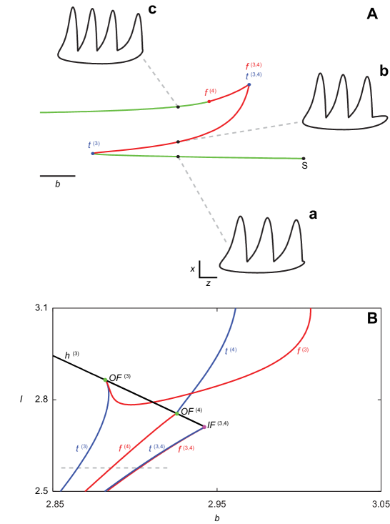
Figure 7: Sketch of the period adding mechanism and corresponding bifurcation curves. In panel A the coloured traces indicate the maximum $z$ coordinate of the solution; colour encodes stability: green is stable, red is unstable. The trajectories a, b and c are projections on the $(z,x)$ plane of the full three-dimensional solution. Panel B shows the actual orbit flip points and the bifurcation curves that take part in the period adding mechanism. The continuation shown in panel A can be obtained by following, for example, the dashed grey line that crosses $t^{(3)}$, $f^{(4)}$, $t^{(3,4)}$ and $f^{(3,4)}$.

3.2 The homoclinic curve $h^{(1)}$

The first characteristic feature of each homoclinic curve $h^{(k)}$ is its U-shape, as qualitatively sketched in Fig. 8 for the lower part of the homoclinic curve $h^{(1)}$ (which curve is depicted only qualitatively). In fact, the U-turn is so sharp that it can be detected only on a very small scale in the parameter space and on any wider scale, as in Fig. 5A, the two branches appear almost as a double cover of the same curve. Note that, as the U is traced, there is a transition between a homoclinic with 1 spike to one with 2 spikes. Such sharp U-turns of homoclinic orbits have been observed in other systems, see e.g. [34, 9], and are typically characterised by orbits gaining an extra spike or pulse. As we shall see, similar U-turns on higher homoclinic branches $h^{(k)}$ cause transitions from $k$- to $(k+1)$-spike homoclinic cycles although, as we shall see, there are important extra details for $k>3$, and the case $k=2$ is special.

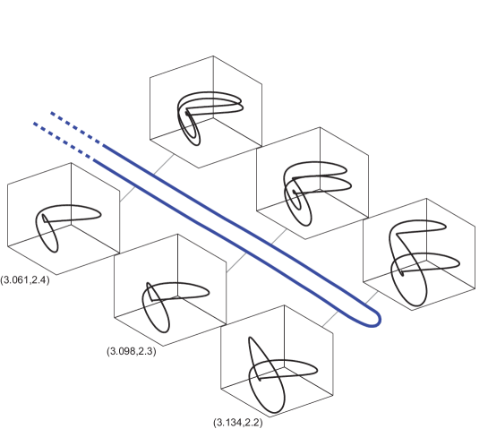
Figure 8: Sketch of a U-shaped homoclinic bifurcation. The $(b,I)$ coordinates are reported near the corresponding 1-spike trajectories on the lower branch of the homoclinic curve. The same values, with the chosen accuracy, hold for the 2-spike trajectories on the upper branch. Adapted from [36], reprinted with permission.

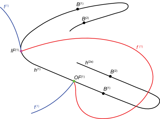
Figure 9: Sketch of $h^{(1)}$: note the presence of just one flip bifurcation ($f^{(1)}$) that connects the inclination flip point $IF^{(1)}$ to the orbit flip point $OF^{(1)}$.

The homoclinic bifurcation curve $h^{(1)}$ is further sketched in Fig. 9. In this and subsequent similar figures bifurcation curves are depicted in an exaggerated way in a pseudo parameter plane in order to elucidate their topological features. The key feature here is an inclination flip point labelled $IF^{(1)}$ that separates two portions of the homoclinic branch, both U-shaped. We shall focus on the lower portion. The inclination flip in this case is of type B according to the classification reported in [25] and [38, Fig.7]; there are single curves of period-doubling and fold of cycle bifurcations emanating from the codimension-two point. Following the branch $h^{(1)}$ away from the inclination flip, we find an orbit flip. Again, two other curves of local bifurcations emanate, a period doubling and a fold. Note how the period-doubling bifurcation $f^{(1)}$ connects the two codimension-two points $IF^{(1)}$ and $OF^{(1)}$, whereas the two fold of cycle curves labelled $t^{(1)}$ are distinct. We also note the presence of Belyakov points, labelled as $B^{(1)}$ on the 1-spike branch $h^{(1)}$ and as $B^{(2)}$ on the 2-spike branch $h^{(2a)}$. Between these two points along the homoclinic curve, the saddle equilibrium is actually a saddle focus (with complex eigenvalues). The real curves are superimposed to the brute-force bifurcation diagram in panel A of Fig. 5. With respect to the sketch, one further period-doubling and two fold of cycles (meeting at a cusp point) curves are displayed (right-bottom corner). One of these fold of cycles is rooted at the Belyakov point $B^{(1)}$.

The numerical continuation suffers convergence problems along the branches of 2-spike homoclinic orbits as they return towards $IF^{(1)}$ and are depicted to end in “mid air”. The eventual fate of the multi-spike branches remains an open issue which we shall not address here, partly because they do not seem to play any further role in the regular-to-irregular bursting transition of interest in this paper.

3.3 The homoclinic bifurcation curves $h^{(k)}$ and their degeneracies

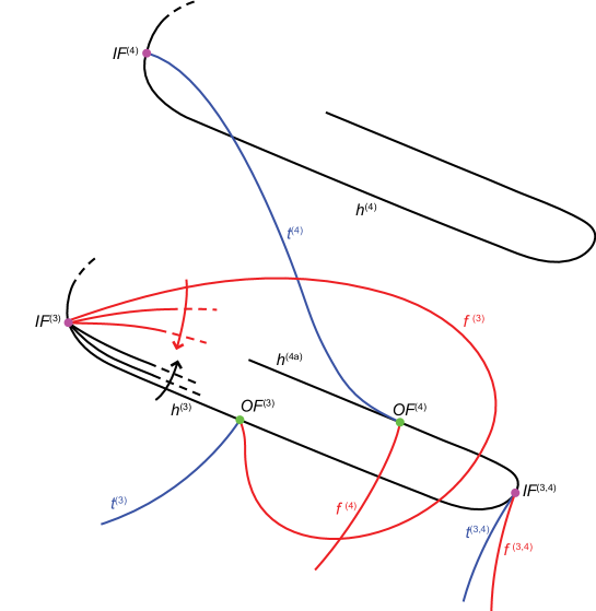
Figure 10: Sketch of the bifurcation structure around the $k$-th homoclinic bifurcation $h^{(k)}$. In this particular sketch, $k=3$, but the general sketch is valid for any $k\geq 3$. For completeness, the sketch also shows the homoclinic curve for $k=4$. This undergoes the same sequence of bifurcations as $h^{(3)}$, which are not depicted.

The qualitative feature of the homoclinic bifurcation curve $h^{(3)}$, which is sketched in Fig. 10, is valid for any $k\geq 3$. The fundamental difference with respect to $h^{(1)}$ is the absence of any Belyakov point. This is due to the fact that the whole homoclinic curve lies in a region of the parameters plane where the eigenvalues of the equilibrium involved in the homoclinic trajectory are real. The curve $h^{(3)}$ emanates from an inclination flip point $IF^{(3)}$, which appears to be distinct from $IF^{(1)}$ but occurs nearby in parameter space. One distinction with the previous case is that the inclination flip is now of type C, which means that an entire period-doubling cascade emanates, as do multiple-pulse homoclinic orbits for all periods ($h^{(3)}$,$h^{(6)}$,$\ldots$). These cascades are illustrated schematically via the sequence of lines superimposed with curved arrows in Fig. 10. We do not focus here on these additional bifurcations. Also, there are again computational difficulties with determining precisely what happens to the branch on the “far” side of $IF^{(3)}$, or of the homoclinic curve $h^{(4a)}$ as it returns towards the vicinity of $IF^{(3)}$. Instead we focus on the transitions that occur close to U-turn as $h^{(3)}$ transitions into $h^{(4a)}$.

Each branch of the $U$-turn undergoes two orbit-flip bifurcations:

• $OF^{(3)}$, where the first bifurcation of the period-doubling cascade ends and meets a fold of cycles (respectively $f^{(3)}$ and $t^{(3)}$ in Fig. 10).

• $OF^{(4)}$, where $t^{(4)}$ and $f^{(4)}$ are rooted: the former is connected with $IF^{(4)}$ on the primary homoclinic bifurcation of the subsequent homoclinic doubling cascade, whereas the latter takes part in the period adding process, as described in Fig. 7.

The real curves are superimposed to the brute-force bifurcation diagram in panel C of Fig. 5.

Very close to the tip of the U-shaped homoclinic bifurcation, there is an additional inclination flip point, labelled $IF^{(3,4)}$ in Fig. 10. From this point, the two curves $t^{(3,4)}$ $f^{(3,4)}$ are born, which are the additional bifurcations that take part in the spike-adding process depicted in Fig. 7. However, we have not been able to numerically detect $IF^{(3,4)}$, due it would seem to the very sharp turn of the homoclinic curve, but we can infer its presence as we now explain. Furthermore, the geometric analysis in Sec. 4 shall provide more careful justification for the presence of this bifurcation.

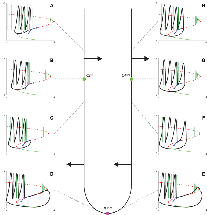
Figure 11: Representation of how the homoclinic trajectories change along the U-shaped homoclinic bifurcation curve. Each panel contains the homoclinic orbit (thick black line) on the plane $(z,x)$ and the results of a bifurcation analysis of the slow-fast subsystem of Eq. (3) (thin coloured lines and dots); the blue arrows are the unstable eigenvectors of the saddle node equilibrium. The arrows in the central panel, on the parameter plane, indicate the direction of bifurcation of periodic orbits from the homoclinic bifurcation curve. For a detailed description of each panel, see the main text.

Figure 11 shows more details of the orbits close to the $U$-turn, which provides further evidence for the presence of the additional inclination flip $IF^{(3,4)}$. In this figure, the central U-shaped curve represents the homoclinic bifurcation, and the eight surrounding panels display the homoclinic trajectories (black thick lines) at significant points on the curve, superimposed onto the bifurcation diagram of the fast subsystem (thin coloured lines and points): these results are similar to those shown in Fig. 3, with the only difference that the periodic solutions of the fast system do not constitute a unique “funnel”, but rather they are separated into two distinct sets, due to the presence of two homoclinic bifurcations in the fast subsystem, at the coordinates where the periodic solutions accumulate. Panels A and H are “above” $OF^{(3)}$ and $OF^{(4)}$, respectively, on opposite branches of the homoclinic curve: in both panels, the homoclinic trajectory leaves the saddle node along the leading unstable direction and returns along the only stable direction after 3 (panel A) or 4 turns (panel H). Panels B and G correspond to the orbit flip points $OF^{(3)}$ and $OF^{(4)}$, respectively: it can be clearly seen how the homoclinic trajectory leaves the saddle node along the non-leading unstable direction. Again, the trajectory returns to the equilibrium point after 3 (panel B) or 4 spikes (panel G). Panels C-F are located between $OF^{(3)}$ and $OF^{(4)}$ and their purpose is to illustrate the qualitative changes that the homoclinic trajectory undergoes between the two orbit flip points and especially near the tip of the homoclinic curve, where we conjecture the presence of the inclination flip point $IF^{(3,4)}$. In particular, in panels C and E it can be observed how the homoclinic trajectory leaves the saddle node again along the leading unstable direction, but this time in the opposite sense than in panels A and H. This makes the homoclinic orbits sort of canard cycles that spend a large amount of time on the unstable part of the slow manifold. In the $0<\mu\ll 1$-regime of the HR model it has been shown that canard trajectories (not specifically homoclinic orbits) of this kind exist for a wide range of parameters, and they are known to be directly involved in the spike adding mechanism [11, 20, 48]. Finally, panels D and E are topologically similar to panels C and F, with the only difference that, being so close to the tip of the homoclinic curve, the canard orbits are maximal: in particular, when the orbit goes past the upper fold of equilibria in the fast subsystem, an additional turn is added to the trajectory, which is the fundamental mechanism behind period adding in this and other models. Numerical evidence shows that this happens exactly at the parameters values corresponding to the tip of the homoclinic bifurcation curve.

The arrows in the central panel of Fig. 11 indicate the direction of bifurcation of periodic orbits from the homoclinic bifurcation curve: the three points $OF^{(3)}$, $OF^{(4)}$ and $IF^{(3,4)}$ divide the homoclinic curve in four distinct regions. By going from one region to the other, the direction of bifurcation of periodic orbits changes, due to the presence of the orbit flip degeneracies and of the turning point at the tip of the U-shaped curve: this gives a first, intuitive, indication that another degeneracy point where the orbit undergoes some switching must be present. There are three such generic codimension-two points that lead to side-switching in the case that the saddle point is a real saddle; orbit flip, inclination flip and resonant eigenvalues. The latter occurs when $\mu_{1}=-\lambda_{1}$, where $\mu_{1}$ is the stable eigenvalue of the saddle point and $\lambda_{1}$ is the weakest unstable eigenvalue. We can easily check that the eigenvalue condition is not satisfied, and we can rule out the presence of an orbit flip, since the direction along which the trajectory leaves the saddle node does not change. Hence we are left only with the possibility that the point at the tip is indeed an inclination flip. A very similar structure has been found in [6, Fig.19] in another context.

3.4 The special case $k=2$

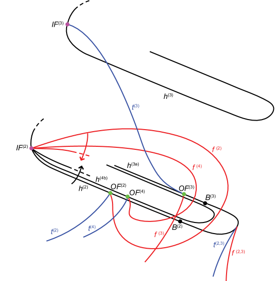
Figure 12: Sketch of $h^{(2)}$: the inclination flip point $IF^{(2)}$ gives birth to both a homoclinic doubling and a period doubling cascade. Note the presence of two Belyakov points, $B^{(1)}$ and $B^{(2)}$.

The homoclinic bifurcation curve $h^{(2)}$ is sketched in Fig. 12 (the real curves were superimposed on the brute-force bifurcation in panel B of Fig. 5). Here we also compute a separate homoclinic curve $h^{(4b)}$ with four spikes that also comes out of the inclination flip point $IF^{(2)}$ (which again appears to be distinct from $IF^{(1)}$ although nearby to it in parameter space). This curve exists because the inclination flip is of type C and is the first in an infinite sequence of the subsidiary homoclinic bifurcations that emanate from the codimension-two point. Like in the general case for $k>2$, each homoclinic branch emanating from the $IF$ has an orbit flip. The fold bifurcation $t^{(2)}$ is the one that is directly involved in the spike-adding from 2 to 3 spikes similarly to what shown in Fig. 7 for the 3 to 4-spikes transition. A connection between the homoclinic curves $h^{(3a)}$ and $h^{(3)}$ is provided by the fold of cycles $t^{(3)}$: this latter bifurcation terminates the chaotic region that is born with the period doubling cascade that starts with $f^{(2)}$, as can be seen in panel B of Fig. 5.

The curves $t^{(2,3)}$ and $f^{(2,3)}$ converge on the tip of the U-turn. Note that there can be no inclination flip in this case, because between the two Belyakov points $B^{(2)}$ and $B^{(3)}$ the equilibrium has complex eigenvalues.

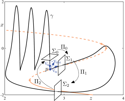
Figure 13: A 3-spike homoclinic orbit $\gamma$ of system (1) projected onto the $(z,x)$-plane and superimposed onto the bifurcation diagram of the fast subsystem. The values of parameters $b$ and $I$ for this orbit correspond to the tip of the homoclinic curve computed in [35] and, hence, to the conjectured inclination flip bifurcation. We also show the saddle equilibrium $p$ together with its strong unstable, weak unstable and stable eigendirections $\mathrm{v}_{\!uu}$, $\mathrm{v}_{\!u}$ and $\mathrm{v}_{\!s}$, respectively. The three cross-sections $\Sigma_{i}$, $i=0,..,2$, allow to construct a return map $\Pi$ from $\Sigma_{1}$ back to itself, in order to study the behaviour of nearby trajectories (for fixed $b$ and $I$ close to the transition of interest).

4 Analysis of inclination flip due to fold in slow manifold

The purpose of this section is to show theoretically the presence of an inclination flip codimension-two point at the sharp turning points of each of the curves $h^{(k)}$ with $k>2$. Moreover, we aim to show that this process is a natural consequence of the sharp folding in the curve of homoclinic orbits, and that this sharp turn is itself a consequence of the canard-related transition of a $n$-spike homoclinic orbit into an $(n+1)$-spike homoclinic orbit. Furthermore, by constructing an approximate return map around the critical homoclinic orbit, we are able to derive asymptotic expressions for the curve of saddle-node of limit cycle bifurcations that emanates from this codimension-two point.

The method of analysis is to construct the return map as a composition of approximate Poincaré maps in a full neighbourhood of both parameter and phase space of the codimension-two point in question; see Fig. 13. The analysis is general and can apply to any three-dimensional system with the same generic features as the HR model. However, the key hypothesis has to be justified numerically (in Subsection 4.1 which follows), namely that the forward image of any smoothly parameterised set of trajectories that interacts transversely with the fold of the critical manifold of the slow-fast system undergoes a sharp fold when viewed in any transverse Poincaré section. This assumption is formalised in the construction of the map $\Pi_{2}$ in Subsection 4.2 below.

4.1 The process of spike-adding

It is useful to examine in detail what happens to the trajectory of the homoclinic orbit as it passes close to the sharp turning point in one of the loops of the loci of homoclinic orbits. Consider Fig. 13 which depicts just such an orbit that is undergoing a transition from three to four spikes at parameter values $b=2.9427488761,I=2.7111448924$. We shall henceforth refer to these as the critical parameter values. Note that the nascent fourth spike forms via the interaction of the unstable manifold with the fold point of the critical manifold (depicted by a dashed red line). Figure 11 shows homoclinic orbits on the branch just before (panel D) and just after (panel E) this critical codimension-two orbit.

Figure 14 and Fig. 15 show the results of a numerical computation of a portion of the unstable manifold of the saddle point at the critical parameter values. The map shown in Fig. 14 (right panel) was computed by variation of a transverse co-ordinate in the unstable manifold close to the equilibrium point $p$ and computing until the first return to a Poincaré section given by $z=2.75$. In particular the set $U_{1}$ of initial conditions chosen was of the form

$$U_{1}=\{(x,y,z)=p+\varepsilon\mathrm{v}_{u}+\theta\mathrm{v}_{uu}|\mbox{ for }\theta\in(-\varepsilon,\varepsilon)\}$$

where $\varepsilon=0.1$ was chosen to give a close approximation to the unstable manifold $W^{u}_{\rm loc}(p)$ in a neighbourhood of the critical homoclinic orbit. Since the unstable manifold is an invariant set, the theory predicts that trajectories that start on the manifold should remain on it indefinitely: unfortunately, due to errors in the numerical integration of this slow-fast system close to the critical manifold, such a result cannot be obtained with standard integration techniques. However, it is possible to overcome this problem by resorting to continuation techniques by setting up a proper boundary value problem (BVP), where one of the parameters that are allowed to vary is the integration time. This particular technique has been exploited, for example, in [13] to compute part of the manifold of the Lorenz system.

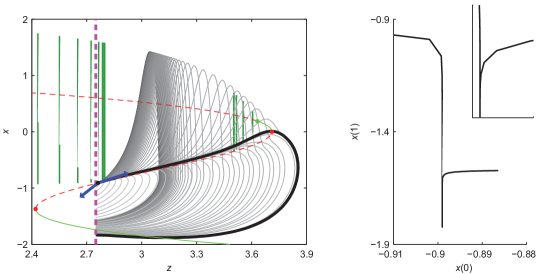
Figure 14: (Left panel) Trajectories in the unstable manifold at the critical parameter values $b=2.9427488761$, $I=2.7111448924$. (Right panel) Approximate 1D map showing that the unstable manifold of the homoclinic trajectory is folded. For a detailed description of each panel, see the main text.

By solving the BVP with AUTO, we can obtain the results shown in Fig. 14. As in previous figures, in the right panel the thin coloured lines represent the bifurcation diagram of the fast subsystem and the blue arrows are the unstable eigenvectors of the saddle node equilibrium. The purple dashed line is the section that constitutes the terminating point of the integrations. The thin grey lines are the integrations of the system obtained by varying the parameter $\theta$ in the range $[-0.1,0.1]$; the thick black line is a piece of the homoclinic trajectory that satisfies the boundary conditions and is used to start the continuation procedure (which corresponds to $\theta\approx-0.001$). The left panel shows an approximate 1D map of the initial versus the final $x$-coordinate. It can be clearly seen that such an approximate map is not invertible (see also the inset, which contains a zoom of the central part), i.e., two distinct initial conditions lead to the same final condition. This constitutes a further justification of our conjecture, since it shows that the unstable manifold of the homoclinic trajectory is folded.

 

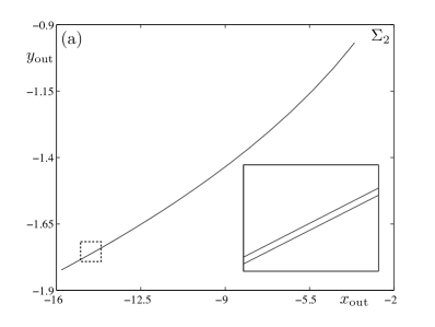
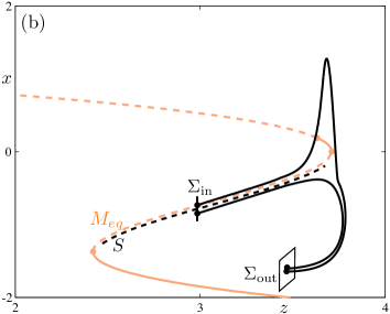
Figure 15: (Panel (a)) Image of the initial conditions $U_{1}$ computed as in Fig. 14 projected onto the $x$ and $y$ co-ordinates of the outgoing Poincaré section $z=2.75$. (Panel (b)) Schematic representation of a general slow-fast system in 3D with a saddle-type slow (Fenichel) manifold $S$ and an underlying critical manifold $M_{eq}$ that is folded. Also shown are two orbit segments with very close initial conditions; only one gets a twist when passing close to the upper fold of $M_{eq}$, due to the relative position of its initial conditions with respect to $S$.

To show this folded manifold in more detail, we depict in Fig. 15 (a) the image of $U_{1}$ in the Poincaré section $z=2.75$. Note the folded shape of the image of $U_{1}$. We conjecture that this fold is a direct consequence of a portion of the unstable manifold passing close to the fold point of the critical manifold $M_{eq}$. This conjecture is confirmed by noting from the computation of the trajectories in question in Fig. 14 that the region of the sharp turning point in the image of $U_{1}$ corresponds to the trajectories that pass the closest to the fold in $M_{eq}$ (actually since Fig. 14 was computed at the critical parameter values, the trajectory that corresponds to the closest point to the fold is on the homoclinic orbit). Similar passage near such a fold of the critical manifold has previously been found in the HR model and has previously been shown to underlie spike-adding at the level of periodic orbits. It was first reported in [48, 49], where the author focused on chaotic dynamics in between $n$-spike and ($n+1$)-spike orbits as well as the disappearance of bursting upon parameter variation. This mechanism has been studied more recently using the framework of slow-fast dynamical systems in [20].

We show in Fig. 15 (b) a schematic representation of the dynamical behaviour suggested by our numerical results. We depict a three-dimensional slow-fast system with all the generic features of the HR model; two fast variables and, hence, a one-dimensional critical manifold $M_{eq}$. The figure shows the projection onto the $(z,x)$-plane, where $z$ is slow and $x$ is fast and we superimpose two segments of trajectories with initial conditions chosen to be very close to one another and to $M_{eq}$. When $M_{eq}$ is cubic-shaped (i.e. with two fold points) and when its middle branch is composed by saddle equilibria of the fast subsystem, then away from the fold points this middle branch perturbs smoothly with respect to the small parameter $\varepsilon$ to a saddle slow (Fenichel) manifold $S$ [16]. In this configuration, one can observe at the level of both transient and long-term dynamics nearby trajectories and attractors that diverge from one another when one gains an extra twist as it passes close to the upper fold of $M_{eq}$ whereas the other does not; see two such orbit segments in Fig. 15. This particular dynamical behaviour can be understood by further looking at the underlying slow-fast structure of the problem. Indeed, the families of (un)stable manifolds $W^{u,s}(p)$ of the saddle equilibria $p$ associated with the fast dynamics perturb smoothly to stable and unstable manifolds $W^{u,s}(S)$ of the Fenichel manifold $S$ [16]. Then, if two sets of initial conditions are taken close to the slow manifold $S$, on opposite sides of the unstable manifold of $S$ will follow $S$ for some time until one jumps down and the other jumps up, hence gaining an extra twist.

Thus, these numerical results provide strong justification that the process of spike adding is caused by the portion of the trajectory of the homoclinic orbit that is closest in time to the local unstable manifold passing close to the fold point of the slow manifold. In turn such a passage causes a sharp fold in the forward image of the local unstable manifold. The aim of the rest of this section is then to argue that this process causes a sharp turning point in parameter space of the locus of homoclinic orbits and that there is necessarily an inclination-flip bifurcation point there. Moreover, a fold curve of periodic orbits and a period doubling bifurcation curve emanate from the inclination flip.

4.2 Construction of Poincaré return map

Consider a sufficiently smooth three-dimensional vector field

$$\dot{x}=f(x,\mu),\qquad x\in\mathbb{R}^{3},\quad\mu\in\mathbb{R}^{2},$$

that has a saddle point $p$ with real eigenvalues $\lambda_{\!uu}>\lambda_{\!u}>0>\lambda_{\!s}$, with corresponding eigenvectors $\mathrm{v}_{\!uu}$, $\mathrm{v}_{\!u}$ and $\mathrm{v}_{\!s}$. We assume for simplicity (after a parameter dependent change of co-ordinates if necessary) that the location of and linearisation at $p$ is parameter independent. Suppose that, at a critical codimension-two point $\mu=0$, a homoclinic orbit $\gamma(t)$ to $p$ exists that satisfies certain non-degeneracy hypotheses:

(H1)

$\gamma(t)\to p$ as $t\to\pm\infty$

(H2)

$\gamma(t)$ is tangent to $\mathrm{v}_{\!u}$ as $t\to-\infty$ and specifically approaches $p$ along the positive $\mathrm{v}_{\!u}$ direction.

We also suppose that the sign of $\mathrm{v}_{\!s}$ has been chosen so that $\gamma(t)$ approaches $p$ along the positive $\mathrm{v}_{\!s}$ direction as $t\to+\infty$.

(H3)

The map $\Pi_{2}$ (defined below) is degenerate such that it can be described by the given quadratic form to leading order.

(H4)

The parameter $\mu$ unfolds this codimension-two singularity in a generic way. (Specific choices for $\mu=(\mu_{1},\mu_{2})$ are defined below.)

We begin the analysis by considering three separate Poincaré sections $\Sigma_{0}$, $\Sigma_{1}$, and $\Sigma_{2}$ as depicted in Fig. 13 for the HR model and in Fig. 16 for a general system.

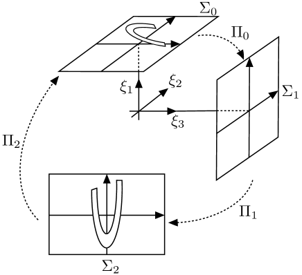
Figure 16: Poincaré sections $\Sigma_{0}$, $\Sigma_{1}$, and $\Sigma_{2}$ for the study of the inclination flip bifurcation in a general three-dimensional system.

The cross-sections $\Sigma_{0}$ and $\Sigma_{1}$ are defined in terms of local coordinates $(\xi_{1},\xi_{2},\xi_{3})$ corresponding to projection along the three-dimensional basis ($\mathrm{v}_{\!s}$, $\mathrm{v}_{\!u}$, $\mathrm{v}_{\!uu}$). Specifically, let

$$\Sigma_{0}=\{(\xi_{1},\xi_{2},\xi_{3})|\xi_{1}=\varepsilon\},\qquad\Sigma_{1}=\{(\xi_{1},\xi_{2},\xi_{3})|\xi_{2}=\varepsilon\}$$

for $0<\varepsilon\ll 1$.

The section $\Sigma_{2}$ is chosen to be transverse to the flow at a point $\gamma(0)$ along the critical homoclinic orbit, at an $O(1)$ distance from $p$. Let local co-ordinates $(\eta_{1},\eta_{2})$ be chosen within $\Sigma_{2}$ such that $\gamma(0)$ is at the origin and the tangent vector to $W^{u}(p)\cup\Sigma_{2}$ at $\gamma_{0}$ lies along the $\eta_{1}$ axis. Furthermore, after a parameter dependent change of co-ordinates if necessary, we shall suppose that the flow from $\Sigma_{1}$ to $\Sigma_{2}$ is independent of the unfolding parameters $\mu$. A convenient choice of unfolding parameters is to assume that the intersection between $\Sigma_{2}$ and the component of the one-dimensional stable manifold $W^{s}(p)$ that corresponds to $\gamma(0)$ when $\mu=0$ is precisely given by $(\eta_{1},\eta_{2})=(\mu_{1},\mu_{2})$. See Fig. 17.

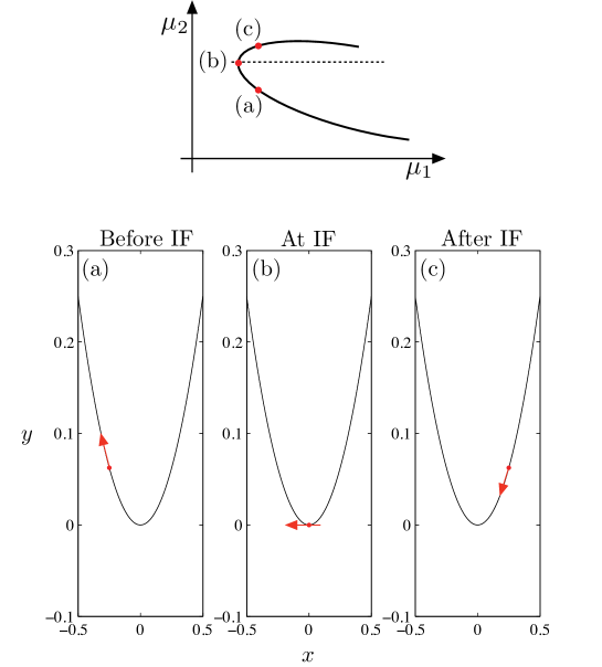
Figure 17: Schematic representation of the return map computed for this system.

We are now in the position to define leading-order Poincaré maps obtained by following trajectories between each of these Poincaré sections. The local map from $\Pi_{0}:\Sigma_{0}\to\Sigma_{1}$ can be obtained by solving the linear equations in a neighbourhood of $p$. It is most useful in what follows to instead deal with $\Pi_{0}^{-1}:\Sigma_{1}\to\Sigma_{0}$. Specifically, to leading order we obtain

$$\Pi_{0}^{-1}:\begin{pmatrix}\xi_{1}\\ \varepsilon\\ \xi_{3}\end{pmatrix}\mapsto\begin{pmatrix}\varepsilon\\ \xi_{2}\\ \xi_{3}\end{pmatrix}=\begin{pmatrix}\varepsilon\\ K_{1}\xi_{1}^{\Delta_{1}}\\ K_{2}\xi_{3}\xi_{1}^{\Delta_{2}}\end{pmatrix},$$

where

$$0<\Delta_{2}=\frac{\operatorname{-}\lambda_{\!uu}}{\lambda_{\!s}}<\Delta_{1}=\frac{\operatorname{-}\lambda_{\!u}}{\lambda_{\!s}},\quad K_{1}=\varepsilon^{1-\Delta_{1}}\quad\mbox{and }K_{2}=\varepsilon^{-\Delta_{2}}$$

Hypothesis (H3) can now be encapsulated in the leading-order expression for the Poincaré map $\Pi_{1}:\Sigma_{1}\to\Sigma_{2}$. We construct this map in two stages. First consider the image of $W^{u}(p)$

$$\begin{pmatrix}\eta_{1}\\ \eta_{2}\end{pmatrix}=\begin{pmatrix}\xi_{3}\\ \beta\xi_{3}^{2}\end{pmatrix}$$

where the unit coefficient of the $\eta_{1}$-term is chosen without loss of generality. Also, the $\eta_{2}$ co-ordinate is chosen so that $\beta>0$. Moreover, the assumption (H3) of a sharp fold in the image of $W^{u}(p)$ implies

$$\beta\varepsilon\gg 1$$ (4)

Thus the leading-order expression for the unit tangent vector to $W^{u}(p)\cap\Sigma$ is

$$\tau(\xi_{3})=\begin{pmatrix}D(\xi_{3})\\ 2\beta\xi_{3}D(\xi_{3})\end{pmatrix},\quad\mbox{where}\quad\quad D(\xi)=\frac{1}{\sqrt{1+4\beta^{2}\xi^{2}}}$$ (5)

from which we obtain that the unit normal (in the sense of positive $\xi_{1}$ co-ordinate) is

$$\tau^{\perp}(\xi_{3})=\begin{pmatrix}-2\beta\xi_{3}D(\xi_{3})\\ D(\xi_{3})\end{pmatrix}$$

Hence, the leading-order expression for the full map $\Pi_{1}$ can be written as

$$\Pi_{1}:\begin{pmatrix}\xi_{1}\\ \varepsilon\\ \xi_{3}\end{pmatrix}\mapsto\begin{pmatrix}\eta_{1}\\ \eta_{2}\end{pmatrix}=\begin{pmatrix}\xi_{3}-2\beta\xi_{1}\xi_{3}D(\xi_{3})\\ \beta\xi_{3}^{2}+\xi_{1}D(\xi_{3})\end{pmatrix}$$

Finally, we suppose that the mapping $\Pi_{2}:\Sigma_{2}\to\Sigma_{0}$ is a diffeomorphism that can be expressed to leading-order by its linear terms.

$$\Pi_{2}:\begin{pmatrix}\eta_{1}\\ \eta_{2}\end{pmatrix}\mapsto\begin{pmatrix}\xi_{2}\\ \xi_{3}\\ \end{pmatrix}=B\begin{pmatrix}\eta_{1}-\mu_{1}\\ \eta_{2}-\mu_{2}\end{pmatrix},$$

where $B=\{b_{ij}\}_{i,j=1,2}$ can be assumed generically to be an invertible matrix with all elements nonzero.

4.3 The inclination-flip bifurcation

In the context of the example system in question, an inclination flip is a codimension-two bifurcation that occurs when a path of homoclinic orbits to $p$ undergoes a change in orientation.

From the construction above, the locus of homoclinic orbits to $p$ in the $\mu$-plane is given to leading order by

$$\mu_{2}=\beta\mu_{1}^{2}$$ (6)

which describes a sharp folded curve pointing along the positive $\mu_{2}$-axis. For parameter values within this curve, the twistedness of the unstable manifold along the homoclinic loop $\gamma$ can be computed by following the tangent vector to the stable manifold around the homoclinic orbit $\gamma(t)$.

Let $(\mu_{1},\mu_{2})$ be a point within the homoclinic locus given by (6) and consider such a tangent vector with initial condition in the positive $\mathrm{v}_{\!uu}$ direction within $\Sigma_{1}$. By construction, the image of this initial condition under $\Pi_{1}$ is the vector $\tau(\mu_{1})$ defined above (Fig. 13). The image of $\tau(\mu_{1})$ under $\Pi_{2}$ is then

$$\hat{\tau}(\mu_{1}):=\begin{pmatrix}(b_{11}+2\beta b_{12}\mu_{1})D(\mu_{1})\\ (b_{21}+2\beta b_{22}\mu_{1})D(\mu_{1})\end{pmatrix}$$

Consider $\hat{\tau}$ for $\mu_{1}=\varepsilon$. To leading-order we find

$$\hat{\tau}(\varepsilon)=\begin{pmatrix}b_{12}\\ b_{22}\end{pmatrix}$$

in which we have used the form of $D$ defined above (5) and the scaling (4). Now, under the non-degeneracy hypothesis that $b_{22}\neq 0$, as $t\to\infty$, the tangent vector will tend to $\mbox{sign}(b_{22})\mathrm{v}_{\!uu}$.

A similar argument shows that $\hat{\tau}$ for $\mu_{1}=-\varepsilon$ along the homoclinic locus maps to leading order to

$$\hat{\tau}(\varepsilon)=\begin{pmatrix}-b_{12}\\ -b_{22}\end{pmatrix}$$

in $\Sigma_{0}$. In turn, this vector tends to $-\mbox{sign}(b_{22})\mathrm{v}_{\!uu}$ as $t\to\infty$.

Hence we have shown that the tangent vector to the homoclinic orbit which is in the positive $\mathrm{v}_{\!uu}$ component as $t\to-\infty$, flips its $\mathrm{v}_{\!uu}$ component as $t\to+\infty$, for $\mu$ varying along the homoclinic locus (6) between $\mu_{1}=\varepsilon$ and $\mu_{1}=-\varepsilon$. This shows that there must be an (at least one) inclination flip somewhere in between. In other words, there must be an orbit flip close to the sharp fold in the homoclinic locus.

4.4 Unfolding the dynamics near the inclination flip

Here we will extend the analysis to provide a local asymptotic prediction of the bifurcations of periodic orbits that emanate from the inclination flip point. To this end we look for fixed points of the return map

$$\Pi_{2}\circ\Pi_{1}\circ\Pi_{0}:\Sigma_{0}\to\Sigma_{0}.$$

In fact, it is most convenient to consider the Poincaré section $\Sigma_{2}$ and seek a condition for a fixed point in the form

$$\Pi_{2}^{-1}\circ\Pi_{0}^{-1}(\xi_{1},\xi_{3})^{T}=\Pi_{1}(\xi_{1},\xi_{3})^{T}.$$

To this end we find

$$\begin{pmatrix}\mu_{1}\\ \mu_{2}\end{pmatrix}+\hat{B}\begin{pmatrix}K_{1}\xi_{1}^{\Delta_{1}}\\ K_{2}\xi_{3}\xi_{1}^{\Delta_{2}}\end{pmatrix}=\begin{pmatrix}\xi_{3}(1-2\beta\xi_{1}D(\xi_{3}))\\ \beta\xi_{3}^{2}+\xi_{1}D(\xi_{3}),\end{pmatrix}$$

where

$$\hat{B}=B^{-1}=\frac{1}{\mbox{ det}(B)}\begin{pmatrix}b_{22}&-b_{12}\\ -b_{21}&b_{11}\end{pmatrix}$$

We now need to analyse these fixed point equations and find fold and flip bifurcations. We suppose we can do a rescaling so that $B=\textrm{Id}$. Then the equations for the fixed points of the return map read

$$\mu_{1}+K_{1}\xi_{1}^{\Delta_{1}} = \xi_{3}-2\beta\xi_{1}\xi_{3}D(\xi_{3})$$

$$\mu_{2}+K_{2}\xi_{3}\xi_{1}^{\Delta_{2}} = \beta\xi_{3}^{2}+\xi_{1}D(\xi_{3}).$$

Given that $\beta$ is assumed to be large ($\beta\varepsilon\gg 1$), we make the following approximation for $\xi_{3}$ such that it is at least of order 1, that is, “non-small”.

$$D(\xi_{3}):=\frac{1}{\sqrt{1+4\beta^{2}\xi_{3}^{2}}}\approx\frac{1}{2\beta|\xi_{3}|}.$$ (7)

The fixed point equations (multiplying the second one by $\xi_{3}$) then reduce to

$$\mu_{1}+K_{1}\xi_{1}^{\Delta_{1}} = \xi_{3}\mp\xi_{1}$$

$$\mu_{2}\xi_{3}+K_{2}\xi_{1}^{\Delta_{2}}\xi_{3}^{2} = \beta\xi_{3}^{3}\pm\frac{\xi_{1}}{2\beta}.$$

We look for $\mu_{1}\operatorname{-}$ and $\mu_{2}\operatorname{-}$ families of fixed point of the previous set of equations with Auto [14]. We fix the signs and continue in $\mu_{1}$ and in $\mu_{2}$ the solutions to the system

$$\mu_{1}+K_{1}\xi_{1}^{\Delta_{1}} = \xi_{3}-\xi_{1}$$

$$\mu_{2}\xi_{3}+K_{2}\xi_{1}^{\Delta_{2}}\xi_{3}^{2} = \beta\xi_{3}^{3}+\frac{\xi_{1}}{2\beta}.$$

We do find saddle-node bifurcations of equilibria which we can continue in two parameter and obtain a curve of fold points in $(\mu_{1},\mu_{2})$-plane. In order to compute the curve of homoclinic bifurcations in this plane, we use the fact that, in the map $\Pi_{2}$, the homoclinic connection corresponds to

$$\eta_{1}=\mu_{1},\;\eta_{2}=\mu_{2}.$$

In the preceding system of equations, this gives:

$$K_{1}\xi_{1}^{\Delta_{1}}=0,\;K_{2}\xi_{1}^{\Delta_{2}}\xi_{3}=0.$$

Hence, we obtain the equation for the homoclinic curve

$$\mu_{1} = \xi_{3}-\xi_{1}$$

$$\mu_{2} = \beta\xi_{3}^{2}+\frac{\xi_{1}}{2\beta\xi_{3}}.$$

We can then compare the computed curve of folds with the curve of homoclinic points and we present the result in figure 18. We obtain a qualitative agreement with the similar curves computed from the HR system. Indeed, the homoclinic curve is folded and, from the tip of that curve, corresponding to the inclination flip bifurcation $I\!F^{(3,4)}$, emanates a curve of fold bifurcation, which corresponds to $f^{(3,4)}$. Note that our numerics is not valid in the vicinity of this tip (dashed circle in figure 18); however, the trend of both the homoclinic and the fold curves outside this small region seems to indicate that they indeed meet at the tip.

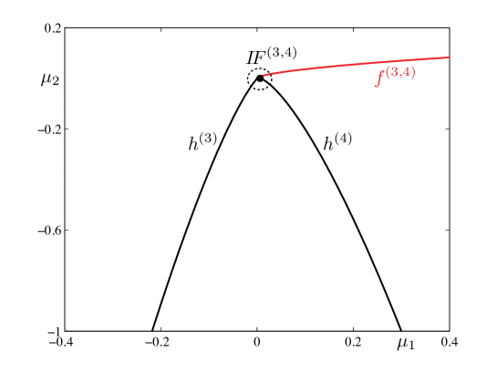
Figure 18: Curve of fold and homoclinic bifurcation points in the $(\mu_{1},\mu_{2})$-plane, obtained from the return map that we derived above.

For values of $I$ and $b$ corresponding to the numerical return map described above and to the inclination flip bifurcation, we can compute the eigenvalue ratios $\Delta_{2}=-\lambda_{\!uu}/\lambda_{\!s}$ and $\Delta_{1}=-\lambda_{\!u}/\lambda_{\!s}$ and check where the point $(\Delta_{2},\Delta_{1})$ is located in the diagram of Fig. 4 (left) in [25], where different unfoldings of the inclination flip bifurcation are studied. It appears that the HR system for the parameter values mentioned above falls into the case C of the classification derived in [25]; therefore, horseshoe dynamics is expected in the vicinity of the inclination flip point, which is consistent with the results of [48].

5 Discussion

This paper has revisited the well-known Hindmarsh-Rose neuron model from a global bifurcation analysis standpoint. To this end, we used different tools, geometrical and numerical. We extracted specific information by relying on the strengths of each method and depicted a global bifurcation scenario by exploiting the tools redundancy to overcome specific weaknesses of each method.

In particular, the analysis we have carried out has shown that numerical continuation based on boundary-value problems can be extremely useful in slow-fast systems where pure simulation can run into difficulties in unfolding bifurcations that are very close to one another. Note also that the homoclinic bifurcations studied here do not themselves represent stable dynamical behaviour. Nevertheless, their influence on the global bifurcation structure is profound.

On the other hand, the geometrical analysis provided details that were not possible to obtain numerically. Moreover, the geometrical analysis points to a generic phenomenon. Namely a sharp fold in the curve of homoclinic orbits in the parameter plane should usually be associated with an inclination flip. Such a phenomenon for example was also observed as part of the unfolding of a tangent period-to-equilibrium heteroclinic cycle [6].

The obtained bifurcation scenario is organised by various curves of homoclinic bifurcations and their codimension-two degeneracies and explains the smooth spike-adding transition (where the number of spikes in each burst is increased by one) typical of the HR model and of many other neuron models. In some sense, the work presented here extends the work of A. Shilnikov who also detected the presence of IF and OF bifurcations in the HR neuron model. He found a wealth of complex dynamics, however, his bifurcation analysis was limited to the curve $h^{(1)}$. The results here have shown that the key to understanding the origins of the spike adding behaviour is to analyse the IFs and OFs occurring on the homoclinic curves $h^{(n)}$ for $n>1$.

The analysis reported in this paper is interesting not only for its intrinsic value in explaining spike-adding in the HR neuron model, but also because similar bifurcation structures have been found and analysed in other studies, such as those reported in [8, 37, 43]. In particular, in [37] the authors perform a bifurcation analysis of a model of pancreatic $\beta$-cells, which show excitable features similar to those of neurons, and find a global bifurcation structure that strikingly resembles what we found for the HR model (see Fig. 4 of the cited paper). In [8, 43], the authors present an analysis of a reduced model of leech heart interneuron: also in this case, the period-adding mechanism is regulated by the presence of homoclinic bifurcations and their degeneracies.

Obviously, a detailed bifurcation analysis of each model will show differences among models, but we dare say that the global bifurcation structure, i.e., the presence of homoclinic bifurcations and the interplay of period doubling and fold of cycles bifurcations, remains unchanged and constitutes a trademark of models of excitable cells that display the widespread period-adding mechanism.

Even if the global bifurcation scenario is quite clear, aspects of the dynamics that remain to be investigated include:

• Further explanation in a neighbourhood of the $IF^{(1)}$ point, in particular whether the $IF^{(n)}$ are really the same bifurcation point or not;

• What happens to the primary homoclinic orbit before $IF^{(1)}$;

• A rigorous analysis using slow-fast methods of the bifurcations caused by the homoclinic orbit passing through a neighbourhood of the fold of the critical manifold;

• Detailed investigation of these phenomena in other models.

Acknowledgement: The research of M.D. was supported by EPSRC under grant EP/E032249/1.

References

- [1] L. A. Belyakov. A case of the generation of a periodic motion with homoclinic curves. Matematiecheskie Zametki, 15:336–341, 1974.
- [2] L. A. Belyakov. The bifurcation set in a system with a homoclinic saddle curve. Matematiecheskie Zametki, 28:910–916, 1980.
- [3] L. A. Belyakov. Bifurcation of systems with homoclinic curve of a saddle-focus with saddle quantity zero. Mathematical Notes, 36:838–843, 1984. 10.1007/BF01139930.
- [4] V. N. Belykh, I. V. Belykh, M. Colding-Jorgensen, and E. Mosekilde. Homoclinic bifurcations leading to the emergence of bursting oscillations in cell models. The European Physical Journal E: Soft Matter and Biological Physics, 3(3):205–219, Nov 2000.
- [5] R. Bertram, M. J. Butte, T. Kiemel, and A. Sherman. Topological and phenomenological classification of bursting oscillations. Bulletin of Mathematical Biology, 57(3):413–439, 1995.
- [6] A. R. Champneys, V. Kirk, E. Knobloch, B. E. Oldeman, and J. D. M. Rademacher. Unfolding a tangent equilibrium-to-periodic heteroclinic cycle. SIAM Journal on Applied Dynamical Systems, 8:1261–1304, 2009.
- [7] A. R. Champneys and Yu. A. Kuznetsov. Numerical detection and continuation of codimension-2 homoclinic bifurcations. International Journal of Bifurcation and Chaos, 4(4):785–822, Aug 1994.
- [8] P. Channell, G. Cymbalyuk, and A. Shilnikov. Origin of bursting through homoclinic spike adding in a neuron model. Physical Review Letters, 98:1–4, 2007. Paper ID 134101.
- [9] O. De Feo, G. M. Maggio, and M. P. Kennedy. The Colpitts oscillator: Families of periodic solutions and their bifurcations. Int. J. Bifurcat. Chaos, 10(5):935–958, May 2000.
- [10] E. de Lange and M. Hasler. Predicting single spikes and spike patterns with the Hindmarsh-Rose model. Biological Cybernetics, 99:349–360, 2008.
- [11] M. Desroches and M. R. Jeffrey. Canards and curvature: the ‘smallness of in slow-fast dynamics. Proceedings of the Royal Society A: Mathematical, Physical and Engineering Science, 467(2132):2404, 2011.
- [12] M. Desroches, B. Krauskopf, and H. M. Osinga. Numerical continuation of canard orbits in slow–fast dynamical systems. Nonlinearity, 23(3):739–765, 2010.
- [13] E. J. Doedel, B. Krauskopf, and H. M. Osinga. Global bifurcations of the Lorenz manifold. Nonlinearity, 19(12):2947–2972, 2006.
- [14] E. J. Doedel and B. E. Oldeman. AUTO-07P: Continuation and Bifurcation Software for Ordinary Differential Equations. Concordia University, Montreal, Quebec, Canada, 2009.
- [15] N. Fenichel. Persistence and smoothness of invariant manifolds for flows. Indiana University Mathematical Journal, 21:193–226, 1971.
- [16] N. Fenichel. Geometric singular perturbation theory for ordinary differential equations. Journal of Differential Equations, 31(1):53–98, 1979.
- [17] M. Golubitsky, K. Josic, and T. J. Kaper. An unfolding theory approach to bursting in fast-slow systems. In H. Broer, B. Krauskopf, and G. Vegter, editors, Global Analysis of Dynamical Systems. Festschrift dedicated to Floris Takens for his 60th birthday, pages 277–308. IOP Publishing, 2001.
- [18] J. M. González-Miranda. Observation of a continuous interior crisis in the Hindmarsh-Rose neuron model. Chaos, 13:845–852, 2003.
- [19] J. M. González-Miranda. Complex bifurcation structures in the Hindmarsh-Rose neuron model. International Journal of Bifurcation and Chaos, 17(9):3071 3083, Sep. 2007.
- [20] J. Guckenheimer and C. Kuehn. Computing slow manifolds of saddle type. SIAM Journal of Applied Dynamical Systems, 8(3):854–79, 2009.
- [21] A. V. M. Herz, T. Gollisch, C. K. Machens, and D. Jaeger. Modeling single-neuron dynamics and computations: a balance of detail and abstraction. Science, 314:80–85, October 2006.
- [22] J. L. Hindmarsh and R. M. Rose. A model of the nerve impulse using two first-order differential equations. Nature, 296:162–164, March 1982.
- [23] J. L. Hindmarsh and R. M. Rose. A model of neuronal bursting using three coupled first order differential equations. Proceedings of the Royal Society of London. Series B, Biological Sciences, 221:87–102, 1984.
- [24] A. L. Hodgkin and A. F. Huxley. A quantitative description of membrane current and its application to conduction and excitation in nerve. J. Physiol.-London, 117(4):500–544, Aug. 1952.
- [25] A. J. Homburg and B. Krauskopf. Resonant homoclinic flip bifurcations. Journal of Dynamics and Differential Equations, 12:4:807–50, 2000.
- [26] A. J. Homburg and B. Sandstede. Homoclinic and heteroclinic bifurcations in vector fields. In F. Takens H. Broer and B. Hasselblatt, editors, Handbook of Dynamical Systems III, pages 379–524. Elsevier, 2010.
- [27] G. Innocenti and R. Genesio. On the dynamics of chaotic spiking-bursting transition in the Hindmarsh–Rose neuron. Chaos: An Interdisciplinary Journal of Nonlinear Science, 19(2):023124, 2009.
- [28] G. Innocenti, A. Morelli, R. Genesio, and A. Torcini. Dynamical phases of the Hindmarsh-Rose neuronal model: Studies of the transition from bursting to spiking chaos. Chaos, 17(4):043128(1–11), Dec. 2007.
- [29] E. M. Izhikevich. Neural excitability, spiking and bursting. International Journal of Bifurcation and Chaos, 10:1171–1266, 2000.
- [30] C. K. R. T. Jones. Geometric singular perturbation theory. In R. Johnson, editor, Dynamical Systems, C.I.M.E Lectures, Montecatini Terme, June 1994, volume 1609 of Lecture Notes in Mathematics, pages 44–120. Springer-Verlag, New York, 1995.
- [31] B. Krauskopf, H. M. Osinga, and J. Galán-Vioque. Numerical continuation methods for dynamical systems. Path following and boundary value problems. Springer-Verlag, 2007.
- [32] M. Krupa and P. Szmolyan. Extending geometric singular perturbation theory to nonhyperbolic points — fold and canard points in two dimensions. SIAM J. Math. Anal., 33(2):286–314, 2001.
- [33] Y. A. Kuznetsov. Elements of Applied Bifurcation Theory. Springer-Verlag, New York, 3rd edition, 2004.
- [34] Y. A. Kuznetsov, O. De Feo, and S. Rinaldi. Belyakov homoclinic bifurcations in a tritrophic food chain model. SIAM Journal of Applied Mathematics, 62:462–487, 2001.
- [35] D. Linaro. Nonlinear Dynamical Systems : Applications to Biological and Electronic Oscillators. University of Genoa, Italy, 2011.
- [36] D. Linaro, F. Bizzarri, and M. Storace. On a piecewise linear approximation of the Hindmarsh-Rose neuron model via genetic algorithms suitable for hardware implementation. Journal of Physics: Conference Series, 138:012011 (1–18), 2008.
- [37] E. Mosekilde, B. Lading, S. Yanchuk, and Yu. Maistrenko. Bifurcation structure of a model of bursting pancreatic cells. BioSystems, 63:3–13, 2001.
- [38] B. E. Oldeman, B. Krauskopf, and A. R. Champneys. Death of period-doublings: locating the homoclinic-doubling cascade. Physica D, 146:100–120, 2000.
- [39] H. M. Osinga and K. T. Tsaneva-Atanasova. Dynamics of plateau bursting depending on the location of its equilibrium. Journal of Neuroendocrinology, 22(12):1301–1314, 2010.
- [40] P. C. Rech. Dynamics of a neuron model in different two-dimensional parameter-spaces. Physics Letters A, 375:1461–1464, 2011.
- [41] J. Rinzel. Bursting oscillations in an excitable membrane model. In Ordinary and partial differential equations: proceedings of the eighth conference held at Dundee, Scotland, June 25-29, 1984, volume 1151, pages 304–316. Springer-Verlag, 1985.
- [42] B. Sandstede. Constructing dynamical systems having homoclinic bifurcation points of codimension two. Journal of Dynamics and Differential Equations, 9:2:269–88, 1997.
- [43] A. Shilnikov, R. L. Calabrese, and G. Cymbalyuk. Mechanism of bistability: Tonic spiking and bursting in a neuron model. Physical Review E, 71:1–9, 2005. Paper ID 056214.
- [44] A. Shilnikov and G. Cymbalyuk. Transition between tonic spiking and bursting in a neuron model via the blue-sky catastrophe. Phys. Rev. Lett., 94(4):048101, Jan 2005.
- [45] A. Shilnikov and M. Kolomiets. Methods of the qualitative theory for the Hindmarsh-Rose model: a case study. a tutorial. International Journal of Bifurcation and Chaos, 18:2141–2168, 2008.
- [46] L. Shilnikov and D. Turaev. Methods of qualitative theory of differential equations and related topics. AMS Transl. Series II, 2000.
- [47] M. Storace, D. Linaro, and E. de Lange. The Hindmarsh-Rose neuron model: bifurcation analysis and piecewise-linear approximations. Chaos: An Interdisciplinary Journal of Nonlinear Science, 18(3):033128, 2008.
- [48] D. Terman. Chaotic spikes arising from a model of bursting in excitable membranes. SIAM Journal of Applied Mathematics, 51(5):1418–50, 1991.
- [49] D. Terman. The transition from bursting to continuous spiking in excitable membrane models. Journal of Nonlinear Science, 2(5):135–182, 1992.
- [50] X.-J. Wang. Genesis of bursting oscillations in the Hindmarsh-Rose model and homoclinicity to a chaotic saddle. Physica D, 62:263–274, 1993. Special Issue on Homoclinic Chaos.