Entanglement of excited states in critical spin chains

Abstract

Rényi and von Neumann entropies quantifying the amount of entanglement in ground states of critical spin chains are known to satisfy a universal law which is given by the Conformal Field Theory (CFT) describing their scaling regime. This law can be generalized to excitations described by primary fields in CFT, as was done in reference Alcaraz et al. (2011), of which this work is a completion. An alternative derivation is presented, together with numerical verifications of our results in different models belonging to the $c=1,1/2$ universality classes. Oscillations of the Rényi entropy in excited states and descendant fields are also discussed.

I Introduction

Entanglement is a fundamental property of quantum states according to which measurements in one of two sub-parts of a quantum system can (immediately) condition the state of the other part, which may be far away in space. This property was at the origin of Einstein’s criticisms to quantum mechanics in his EPR article in 1935. Today, entanglement is one of the most studied topics in physics and many research lines are related to this concept. It is the property that makes possible quantum computation, teleportation and quantum information processing Nielsen and Chuang (2004). On the other hand, the irruption of quantum information methods and concepts in the condensed matter physics community has led to one of the most fruitful research areas of the last decade Amico et al. (2008). Measurements of entanglement between spatial or more abstract parts of many-body systems and statistical models in their ground state have been proved to unveil essential information characterizing their phases. After all, quantum correlations, or entanglement, in ground states (gs) of many-body systems are responsible for the onset of coherent phases of matter at zero temperature such as superconductivity and Hall states. Probably the most studied quantity in this context is the amount of entanglement between two spatially separated parts of an extended system. Calling $A$ one of these parts, the reduced density matrix, $\rho_{A}$, of the ground state under study, is obtained by tracing the degrees of freedom of the complementary of $A$. If $A$ results in a mixed (pure) state, then $A$ and its complementary are said to be in an entangled (product) state, the amount of entanglement being normally quantified via the von Neumann entropy of $\rho_{A}$:

$$S_{1}(A)=-\mbox{tr }\rho_{A}\ln\rho_{A},$$ (1)

called entanglement entropy. Alternatively, the $n$-th order Rényi entropy is used, $n>1$: $S_{n}(A)=\frac{1}{1-n}\ln\mbox{tr}_{A}\,{\rho_{A}}^{n}$, which contains information on the spectrum of $\rho_{A}$, the entanglement entropy being $\lim_{n\to 1}S_{n}$. The interest of these quantities is threefold. Firstly because of the area law satisfied by (1) (see references in Eisert et al. (2010)), stated in its first version by Bombelli et al in 1986 and by Srednicki in 1993 for a free scalar field, and related to the problem of information loss in black holes Bombelli et al. (1986),Srednicki (1993). Roughly speaking, it states that ground states of Hamiltonians with short-range interactions are such that their entanglement entropy is proportional to the area of the hyper-surface separating $A$ from the rest of the system, hence proportional to $\ell^{d-1}$ in $d$ dimensions, if $\ell$ is the linear size of $A$. This important property serves to characterize the very small fraction of the Hilbert space accessibly to “physical” ground states. In one spatial dimension (1D), the area law implies that the entropy of massive ground states is bounded and independent of the length $\ell$ of the linear part, or block, $A$. Being the entanglement entropy proportional to the minimum amount of information needed to describe the partition $A$, this was used (see references in Cirac and Verstraete (2009)) to interpret the efficiency of the Density Matrix Renormalization Group (DMRG) algorithm in massive phases White (1992), and the lack of this efficiency when dealing with gapless phases, a case in which the area law is to be corrected with a logarithmic term in one dimension, leading to an unbounded entropy in infinite systems. In the same spirit, measurements of entanglement are essential in the development of novel Cirac and Verstraete (2009) efficient algorithms for the simulation of quantum many-body systems in one and two dimensions. Entanglement measurements, from a broader perspective, may provide relevant information about the physics of the system under study. Just to give an example that will be cited in the body of the article, the oscillations of the Rényi entropy in critical 1D chains have been proved Calabrese et al. (2010) to be related to the Luttinger parameter entering in their continuum description, which, in principle, could be inferred in this way through quantum information measurements in particular finite-size models.
Finally, the interest of entanglement entropy comes also from the fact that the mentioned logarithmic behaviour of the entanglement in 1D has been proved to be a universal property of critical systems, captured, among other properties of entanglement, by their underlying Conformal Field Theory (CFT). Since the work of Polyakov et. al. Belavin et al. (1984), conformal symmetry of critical two-dimensional systems has been exploited to infer the universal form of correlators, finite size scaling of energy and momentum, critical exponents and several properties of stochastic evolution of interfaces Mussardo (2009); Cardy (2005). Moreover, in 1994, Holzhey et. al., and Calabrese et. al. in 2004 showed in a CFT context that, in a system of length $N$ and periodic boundary conditions (PBCs), the Rényi entropy takes the universal form Holzhey et al. (1994),Vidal et al. (2003),Calabrese and Cardy (2004):

$$S_{n}^{\rm gs}(\ell)=\frac{c\;(n+1)}{6n}\ln\left[\frac{N}{\pi}\sin\left(\frac{\pi\ell}{N}\right)\right]+\gamma_{n}$$ (2)

where $c$ is the central charge of the CFT describing the system scaling limit and $\gamma_{n}$ is a non-universal constant. This statement was generalized to account not only for the ground state entropy but also for low-energy excitations in reference Alcaraz et al. (2011), a generalization which supposes a further prediction of CFT in the field of quantum critical phenomena. By conformal invariance, the finite-size spectrum at criticality has a universal structure determined by the Virasoro algebra satisfied by the generators of the conformal transformations. Each state in the low-energy spectrum exhibits an energy and momentum finite-size scaling determined by the conformal weights, or, roughly speaking, the eigenvalues of the Virasoro operators of the given state. In the same spirit, in reference Alcaraz et al. (2011) it was proved that the Rényi entropy of excitations defined by primary fields are universally related to conformal properties of the operator defining the targeted excitation. In particular, consider the quantity:

$$F^{(n)}_{\Upsilon}\equiv\exp\left[(1-n)(S_{n}^{\Upsilon}(x)-S_{n}^{\rm gs}(x))\right],$$ (3)

defined in reference Alcaraz et al. (2011). It quantifies the excess of entanglement of a state $|\Upsilon\rangle$ related to the primary field $\Upsilon$, with respect to the gs. This quantity Alcaraz et al. (2011) related to the $2n$-point correlator of the operator $\Upsilon$ and its conjugate $\Upsilon^{\dagger}$ in the cylinder:

$$F^{(n)}_{\Upsilon}(x)=n^{-2n(h+\bar{h})}\,\frac{\langle\prod_{j=0}^{n-1}\Upsilon(\frac{2\pi j}{n})\,\Upsilon^{\dagger}(\frac{2\pi(j+x)}{n})\rangle_{\rm cy}}{\langle\Upsilon(0)\,\Upsilon^{\dagger}(2\pi x)\rangle_{\rm cy}^{n}}.$$ (4)

This is the main result we will alternatively derive in the following section, and that will be numerically checked in subsequent sections for different models.
Entanglement of excited states has been also considered in Alcaraz and Sarandy (2008), where universal scaling of the negativity of excitations in the $XXZ$ critical chain was shown. In Masanes (2009) it was shown that a violation of the area law should be expected for the low lying excited states of critical chains, and in Alba et al. (2009) it was considered the entanglement of very large energy excitations in the $XY$ and $XXZ$ models. In Calabrese et al. (2011a),Calabrese et al. (2011b), the law (4) was applied to study systems with continuous degrees of freedom, where it turned to be an accurate description of the finite-size system entanglement.
The aim of this work is to complete the results of reference Alcaraz et al. (2011). In section II an overview of entanglement of excitations in the $XX$ model is given. Section III is a derivation of our results in the framework of the Calabrese and Cardy computation Calabrese and Cardy (2004) (in Alcaraz et al. (2011), the approach of Holzhey et al. (1994) was used instead). Section IV presents some of our results for the bosonic theory and some numerical illustrations for three models in this universality class: the $XX$ (free fermions), $XXZ$ and excluded-volume-$XX$ spin chains. The section concludes with a study of the Rény entropy oscillations in this theory. Section V is a study of the free Majorana CFT with numerical tests in the quantum critical Ising chain. A discussion about the entropy of descendant fields is given in section VI.

II A first sight on entanglement of excitations in the $XX$ model

As a first illustration of the behaviour exhibited by block entanglement in excited states of spin chains, let us consider the $XX$ model for $N$ interacting spins occupying the positions of an $N$-site lattice and whose interaction is defined by the Hamiltonian:

$$H_{XX}=-\frac{1}{2}\sum_{j=1}^{N}\left(\sigma_{j}^{x}\sigma_{j+1}^{x}+\sigma_{j}^{y}\sigma_{j+1}^{y}\right),$$ (5)

where $\sigma_{j}$ are the spin Pauli matrices acting on the $j$-th spin. This well-known model Lieb et al. (1961) is a paradigm of spin chain describing quantum magnetism, it also emerges as the strong on-site repulsion limit of the boson Hubbard model. As discussed in appendix A and in reference Lieb et al. (1961), the $XX$ model is integrable and it can be mapped, through a Jordan-Wigner transformation, into a problem of lattice free fermions. According to such a mapping, the spectrum of the Hamiltonian (5) coincides with the spectrum of a free-fermionic Hamiltonian:

$$H=\sum_{j\in\Omega}E_{j}\,d_{j}^{\dagger}d_{j}+\rm{constant}$$ (6)

where $\{d_{j},d^{\dagger}_{j^{\prime}}\}=\delta_{j,j^{\prime}}$, are the creation and destruction operators of fermions with momentum $k_{j}=2\pi j/N$, $E_{j}=-\cos k_{j}$ is the free-fermionic dispersion relation, and $\Omega$ is a set of $N$ integers or half-integers such that the resulting momenta $k_{j}$ are the ones determined by the periodicity or anti-periodicity of the boundary conditions in the fermionic problem. In other words: each one of the $2^{N}$ eigenstates of (5) is associated with one of the $2^{N}$ fermionic eigenstates of (6):

$$\prod_{j=1}^{n_{F}\leq N}d_{m_{j}}^{\dagger}|0\rangle$$ (7)

(being $|0\rangle$ the fermionic vacuum annihilated by the $d$’s and $\{m_{j}\}_{j=1}^{n_{F}}\equiv\mathbf{K}\subset\Omega$, one of the $2^{N}$ subsets of $\Omega$), and the association is such that the eigenvector in correspondence with the momentum set $\mathbf{K}$ has energy eigenvalue: $E=-\sum_{j\in\mathbf{K}}\,\cos k_{j}$. As explained in the appendix, the Jordan-Wigner transformation is such that a fermion Hamiltonian with anti-periodic boundary conditions (APBCs) is related to the Hamiltonian (5) with periodic boundary conditions (PBCs) for even $n_{F}$, and with APBCs for odd $n_{F}$. We will impose APBCs to the fermions. The corresponding $\Omega$ is:

$$\Omega=\left\{\pm\frac{1}{2},\pm\frac{3}{2},\ldots,\pm\frac{N-1}{2}\right\}.$$ (8)

In this framework, one has that the ground state of (5) corresponds to the Fermi state of (6) with $n_{F}=N/2$ fermions:

$$|n_{F}\rangle=\prod_{0<j\,\leq\,(n_{F}-1)/2}d^{\dagger}_{j}d^{\dagger}_{-j}|0\rangle.$$ (9)

From now on we will denote $|m\rangle$ the Fermi state of $m$ fermions, as in equation (9) (even $m$ is supposed). Let us now consider some low-energy excitations in this model. Due to the conformal invariance, the low-energy excitations present an excess of energy with respect to the ground state which is: $2\pi\Delta/N$, being $\Delta$ the conformal dimension of the excitation. The excess of energy vanishes in the large-$N$ limit: the model is critical. As a critical model, its ground state $|N/2\rangle$ satisfies the law (2), one can ask whether the entropy of low-energy excitations coincides with the gs entropy in the thermodynamic limit, as happens for the energy. It turns out that there is a class of low-energy excitations for which this is indeed true. This type of excitations will be called compact since, as the ground state, they do not exhibit holes in momentum space or, in other words, for them the set $\mathbf{K}$ is composed of consecutive momentum quanta differing by $2\pi/N$. Otherwise the excitations will be called non-compact, and they are such that their entropy is larger than that of the ground state. In what follows we illustrate with examples how excitations in the compact class presents an entropy equal to the gs entropy, up to the oscillations described in Calabrese et al. (2010), with the same non-universal constant $\gamma_{n}$. Afterwards, some non-compact states will be analyzed. These results will be justified with CFT arguments in section IV.
As a first example of compact states we consider the excitation obtained by removing the highest momentum fermion in the $XX$ model, or $d_{n_{F}/2-1/2}|n_{F}>$, with $n_{F}=N/2$. In figure 1 we present the $n=2,3,4$-Rényi entropy of such a state (which is labelled as ($a$)), together with the ground state entropy. The different behaviour of the oscillations (which are present only for $n>1$, and absent in the $N\to\infty$ limit) is the only difference between ground and excited state entropies. As a further illustration, we present the state obtained adding a fermion below the left Fermi point and another one above the right Fermi point (i.e., the state $d^{\dagger}_{n_{F}/2+1/2}\,d^{\dagger}_{-n_{F}/2-1/2}|n_{F}\rangle$). This state is labelled as $(b)$ in figure 1. A final example of compact states is provided by the Umklapp excitation (c.f. table 1), consisting in moving the fermion with most negative momentum to the right of the positive Fermi point, i.e. to $d_{-(n_{F}-1)/2}\,d^{\dagger}_{(n_{F}+1)/2}|n_{F}\rangle$. This can be provedAlcaraz et al. (2011) to have exactly the same entropy $S_{n}$ as the ground state for all values of $n$ (with exactly the same excitations), since such a shift in momentum space $k\to k+2\pi/N$ amounts to a phase shift of the wave-function in position space, leaving the reduced density matrix unchanged.
For the sake of clarity let us introduce the following notation: $(h_{1}\,h_{2}\,\cdots\,:p_{1}\,p_{2}\,\cdots)$ refers to a chiral excitation with holes in the $h_{j}$’s allowed momentum values below the right Fermi point and particles in the $p_{j}$’s momentum values above it, i.e., to the state:

$$\prod_{j,k}d^{\dagger}_{\frac{n_{F}-1}{2}+p_{j}}d_{\frac{n_{F}+1}{2}-h_{k}}|n_{F}\rangle,$$

in such a way that the ground state is denoted as $(\,:\,)$ and the ($a$) excitation is $(1:\,)$.

name of excitation	field	$(h,\bar{h})$	state ($n_{F}=N/2$)	$(h:p)$	$N=8$ example
ground state	$\mathbf{1}$	(0,0)	$|n_{F}\rangle$	$(\,:\,)$	$\circ\circ\bullet\bullet\bullet\bullet\circ\circ$
$(a)$	$e^{-i\phi}$	(1/2,0)	$d_{(n_{F}-1)/2}|n_{F}\rangle$	$(1:\,)$	$\circ\circ\bullet\bullet\bullet\circ\circ\circ$
$(b)$	$e^{i\phi+i\bar{\phi}}$	$(1/2,1/2)$	$d^{\dagger}_{n_{F}/2+1/2}\,d^{\dagger}_{-n_{F}/2-1/2}|n_{F}\rangle$		$\circ\bullet\bullet\bullet\bullet\bullet\bullet\circ$
Umklapp	$e^{i\phi-i\bar{\phi}}$	$(1/2,1/2)$	$d_{-(n_{F}-1)/2}\,d^{\dagger}_{(n_{F}+1)/2}|n_{F}\rangle$		$\circ\circ\circ\bullet\bullet\bullet\bullet\circ$
particle-hole	$i\partial\phi$	$(1,0)$	$d_{(n_{F}-1)/2}\,d^{\dagger}_{(n_{F}+1)/2}|n_{F}\rangle$	$(1:1)$	$\circ\circ\bullet\bullet\bullet\circ\bullet\circ$
R-L particle-hole	$\bar{\partial}\bar{\phi}\partial\phi$	$(1,1)$	$\begin{subarray}{c}d_{(n_{F}-1)/2}\,d^{\dagger}_{(n_{F}+1)/2}\\ d_{-(n_{F}-1)/2}\,d^{\dagger}_{-(n_{F}+1)/2}|n_{F}\rangle\end{subarray}$		$\circ\bullet\circ\bullet\bullet\circ\bullet\circ$
	-	-	$d_{(n_{F}-1)/2}\,d^{\dagger}_{(n_{F}+3)/2}|n_{F}\rangle$	$(1:2)$	$\circ\circ\bullet\bullet\bullet\circ\circ\bullet$

Table 1: A summary of the mentioned excitations. The horizontal line separates the compact states from the non-compact ones. The notation $(h,p)$ applies only for chiral excitations, and the corresponding conformal fields are shown for primary states only.

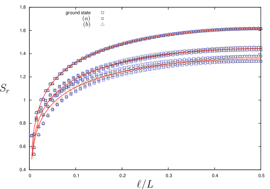
Figure 1: Rényi entropy $S_{r}$, $r=2,3,4$ for three states in the $XX$ model with $N=200$ sites. The states $(a)$ and $(b)$ are described in the text and in table 1. The continuous curves are the universal function (2).

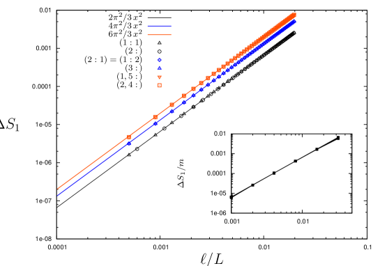
Figure 2: Low-$\ell/N$ behaviour of the excess of von Neumann entropy of different states with $\bar{h}=0$ in the $XX$ model. Continuous lines are equation (10). States with the same value of $h$ have a common color. System sizes are $N=10^{4}$. Inset: several states with $h=m$ ($m$ from 1 to 14) of a $N=8000$ system are shown to satisfy (10).

We will now focus in non-compact excitations, such that holes are created in momentum space. These states do not obey the law (2). The lowest excitation of the $XX$ model with non-zero momentum has excess of energy and momentum equal to $2\pi/N$, and in the fermionic language it corresponds to the destruction of the fermion below the Fermi point and the creation of a fermion immediately above it. In other words, it is the $(1:1)$ state. We will call this excitation a particle-hole excitation. This state is found to exhibit excess of entanglement $\Delta S(\ell)=S(\ell)-S^{\rm gs}(\ell)$ which is larger than zero. Figure 2 represents the $\ell/N<<1$ regime of the excess of entanglement entropy for such a state, together with other particle-hole like excitations. Since the works Holzhey et al. (1994); Vidal et al. (2003); Calabrese and Cardy (2004), one knows that, for small $\ell/N$, the ground state of a critical system satisfies $S_{1}(\ell)\sim\frac{c}{3}\,\ln\ell$. For excited states in the $XX$ model, one observes a correction of the type Alcaraz et al. (2011):

$$\Delta S_{1}(\ell)=\frac{2\pi^{2}}{3}\,(h+\bar{h})\,\left(\frac{\ell}{N}\right)^{2}+O\left[(\ell/N)^{4}\right]$$ (10)

where $\Delta S_{1}$ is the excess of entropy with respect to the ground state and $h$, $\bar{h}$ are the conformal weights of the operator corresponding to the excitation (equation (10) will be justified in section IV). As a further example consider the state $d_{(n_{F}-1)/2}\,d^{\dagger}_{(n_{F}-1)/2+m}|n_{F}\rangle$, such that the fermion nearest to the Fermi point has been displaced $m$ momentum quanta to the right. On inset of figure 2, one observes for this state how curves for different $m$ collapse when the quantity $\Delta S_{1}/m$ is plotted, confirming also in this case the law (10) with $h=m$, $\bar{h}=0$.
It is worth to stress that although some of the states studied in figure 2 present the same low-$x$ dependence of their entanglement and Rényi entropies, their entropy do not coincide for larger values of $x$ in general. This is illustrated in figure 3, in which we show the function $F^{(n)}$ defined in (3) for the excitations studied in figure 2.
In section IV we will show how some of the results presented in this section can be justified with CFT arguments.

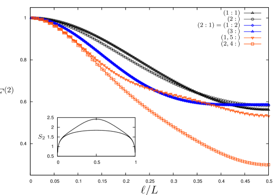
Figure 3: The function $F^{(2)}$ for the same excitations of figure 2 in systems with $N=500$ sites. The inset shows $S_{2}$ for the ground and (1:1) states.

III CFT approach to the entropy of primary fields

In reference Alcaraz et al. (2011) we obtained a general formula for the Rényi entropy of excited states in CFT following the approach of Holzhey, Larsen and Wilczek (HLW) who computed the entanglement entropy of the ground state of CFT systems with periodic boundary conditions. The HLW approach was later generalized by Cardy and Calabrese (CC) to deal with more general situations, as finite temperature, open boundary conditions and several disjoint intervals. It is thus of great interest to re-derive the result of reference Alcaraz et al. (2011) using the CC approach. This is the aim of this section.
Let us start by briefly recalling the main steps of the CC approach. The general set up of the problem is a lattice 1+1 quantum field theory with local commuting observables $\{\hat{\phi}(x)\}$ with eigenvalues $\{\phi(x)\}$ and Hamiltonian $\hat{H}$. The thermal state $\rho$ at inverse temperature $\beta$ has matrix elements

$$\langle\{\phi^{\prime\prime}(x^{\prime\prime})\}|\rho|\{\phi^{\prime}(x^{\prime})\}\rangle=\frac{1}{Z(\beta)}\langle\{\phi^{\prime\prime}(x^{\prime\prime})\}|e^{-\beta\hat{H}}|\{\phi^{\prime}(x^{\prime})\}\rangle$$ (11)

where

$$Z(\beta)={\rm Tr}\,e^{-\beta H}$$ (12)

is the partition function. Equation (11) can be expressed in terms of an euclidean path integral as

$$\langle\{\phi^{\prime\prime}(x^{\prime\prime})\}|\rho|\{\phi^{\prime}(x^{\prime})\}\rangle=\frac{1}{Z(\beta)}\int[d\phi(x,\tau)]\prod_{x}\delta(\phi(x,-\beta/2)-\phi^{\prime}(x^{\prime}))\prod_{x}\delta(\phi(x,\beta/2)-\phi^{\prime\prime}(x^{\prime\prime}))\,e^{-S_{E}}$$ (13)

where $S_{E}=\int_{-\beta/2}^{\beta/2}d\tau\,L_{E}$ with $L_{E}$ the euclidean Lagrangian. The normalization factor in (11) guarantees that ${\rm Tr}\,\rho=1$. The partition function $Z(\beta)$ is obtained doing the path integral with the identification $\phi^{\prime}(x)=\phi^{\prime\prime}(x)$ at $\tau=-\beta/2$ and $\tau=\beta/2$, and integrating over these variables. The geometry of the integration surface is a cylinder of length $\beta$.

Let us now take a system $A$ given by the interval $(u,v)$. One wants to compute the reduced density matrix $\rho(A)$ by tracing over the points not in $A$, that we call $B$. This operation amounts to gluing those points in (13) and doing the integral over them. The effect is to leave a cut $(u,v)$ along the line $\tau=-\beta/2$. To compute ${\rm tr}\,\rho^{n}(A)$ one uses the replica trick. One first makes $n$ copies of (13), labelled by $k=0,\dots,n-1$ and glue them together cyclically

$$\phi^{\prime}_{k}(x)=\phi^{\prime\prime}_{k+1}(x),\quad(k=0,\dots,n-2),\qquad\phi^{\prime}_{n-1}(x)=\phi^{\prime\prime}_{0}(x),\qquad\forall\,x\in A$$ (14)

The path integral on this $n$-sheeted geometry is denoted as $Z_{n}(A)$ and hence

$${\rm tr}\,\rho^{n}(A)=\frac{Z_{n}(A)}{Z(\beta)^{n}}$$ (15)

CC argue that the LHS of (15) is analytic for all $\Re\,n>1$ and that its derivative respect to $n$ in the limit $n\rightarrow 1^{+}$ gives the entropy

$$S_{A}=-\lim_{n\rightarrow 1}\frac{\partial}{\partial n}\frac{Z_{n}(A)}{Z(\beta)^{n}}$$ (16)

Alternatively, one can define the Rényi entropy $S_{n}(A)$ for the interval $A$,

$$S_{n}(A)=\frac{1}{1-n}\log{\rm tr}\,\rho^{n}(A)$$ (17)

and compute the entanglement entropy as

$$S_{A}=\lim_{n\rightarrow 1}S_{n}(A).$$ (18)

Let us now turn to the excited states in CFT that correspond to primary states. If $|0\rangle$ is the vacuum state then the incoming state generated by a primary operator $\Upsilon(z,\bar{z})$, with conformal weights $h$ and $\bar{h}$, is given by

$$|\Upsilon\rangle=\lim_{z,\bar{z}\rightarrow 0}\Upsilon(z,\bar{z})\,|0\rangle$$ (19)

while the outgoing state is given by

$$\langle\Upsilon|=\lim_{z,\bar{z}\rightarrow 0}\bar{z}^{-2h}\,z^{-2\bar{h}}\langle 0|\Upsilon^{\dagger}\left(\frac{1}{\bar{z}},\frac{1}{z}\right)$$ (20)

where $\Upsilon^{\dagger}$ is the operator conjugated to $\Upsilon$, i.e., $\Upsilon\times\Upsilon^{\dagger}={\bf I}+\cdots$. In the latter two equations we have used the radial quantization so that $z=0$ and $z=\infty$ correspond to the infinite past and infinite future respectively. The primary operator corresponding to the vacuum $|0\rangle$ is, of course, the identity, i.e. $\Upsilon={\bf I}$. The density matrix of the ground state is given by the limit $\beta\rightarrow\infty$ of equation (13), which we write as

$$\langle\{\phi^{\prime\prime}(x^{\prime\prime})\}|\rho_{\bf I}|\{\phi^{\prime}(x^{\prime})\}\rangle=\frac{1}{Z}\int[d\phi(x,\tau)]\prod_{x}\delta(\phi(x,-\infty)-\phi^{\prime}(x^{\prime}))\prod_{x}\delta(\phi(x,\infty)-\phi^{\prime\prime}(x^{\prime\prime}))\,e^{-S_{E}}$$ (21)

where $Z=\lim_{\beta\rightarrow\infty}Z(\beta)$ and the action $S_{E}$ is computed over a cylinder of infinite length. Based on equations (19) and (20) we find the following expression for the density matrix of the primary state $|\Upsilon\rangle$,

$$\langle\{\phi^{\prime\prime}(x^{\prime\prime})\}|\rho_{\Upsilon}|\{\phi^{\prime}(x^{\prime})\}\rangle=C\int[d\phi(x,\tau)]\prod_{x}\delta(\phi(x,-\infty)-\phi^{\prime}(x^{\prime}))\prod_{x}\delta(\phi(x,\infty)-\phi^{\prime\prime}(x^{\prime\prime}))\Upsilon(0,-\infty)\,\Upsilon^{*}(0,\infty)\,e^{-S_{E}}$$ (22)

which reduces to (21) for $\Upsilon={\bf I}$. In this equation we have parametrized the primary fields in terms of the space-time coordinates, i.e. $\Upsilon(\sigma,\tau)$, etc. not with the radial coordinates, i.e. $\Upsilon(z,\bar{z})$, as in equations (19) and (20), but there is a one-to-one correspondences between the two. $C$ is a constant which will be fixed below. Following the same steps as for the derivation of equation (15), one finds that the trace of the reduced density matrix $\rho^{n}_{\Upsilon}(A)$ is given by

$${\rm tr}\,\rho^{n}_{\Upsilon}(A)=C^{n}Z_{n}(A)\langle\Upsilon_{0}(0,-\infty)\,\Upsilon^{\dagger}_{0}(0,\infty)\dots\Upsilon_{n-1}(0,-\infty)\,\Upsilon^{\dagger}_{n-1}(0,\infty)\rangle_{{\cal R}_{n}}$$ (23)

where ${\cal R}_{n}$ is the $n$-sheeted Riemann surface that results from the sewing of the $n$ copies of the original cylinder along the cuts associated to the interval $A$. The label $k=0,\dots,n-1$, of the primary field $\Upsilon_{k}$, and its conjugate $\Upsilon_{k}^{\dagger}$, denotes the sheet they belong to. The constant $C$ can now be fixed imposing the normalization of the reduced density matrix,

$${\rm Tr}\,\rho_{\Upsilon}(A)=CZ\langle\Upsilon_{0}(0,-\infty)\,\Upsilon^{\dagger}_{0}(0,\infty)\rangle_{{\cal R}_{1}}=1$$ (24)

Eliminating $C$ from this equation and plugging its value into (23) yields

$${\rm tr}\,\rho^{n}_{\Upsilon}(A)=\frac{Z_{n}(A)}{Z^{n}}\frac{\langle\Upsilon_{0}(0,-\infty)\,\Upsilon^{\dagger}_{0}(0,\infty)\dots\Upsilon_{n-1}(0,-\infty)\,\Upsilon^{\dagger}_{n-1}(0,\infty)\rangle_{{\cal R}_{n}}}{\langle\Upsilon_{0}(0,-\infty)\,\Upsilon^{*}_{0}(0,\infty)\rangle_{{\cal R}_{1}}^{n}}$$ (25)

Finally, using equation (15) in the limit $\beta\rightarrow\infty$, one gets

$$F^{(n)}_{\Upsilon}(A)\equiv\frac{{\rm tr}\,\rho^{n}_{\Upsilon}(A)}{{\rm tr}\,\rho^{n}_{\bf I}(A)}=\frac{\langle\Upsilon_{0}(0,-\infty)\,\Upsilon^{\dagger}_{0}(0,\infty)\dots\Upsilon_{n-1}(0,-\infty)\,\Upsilon^{\dagger}_{n-1}(0,\infty)\rangle_{{\cal R}_{n}}}{\langle\Upsilon_{0}(0,-\infty)\,\Upsilon^{\dagger}_{0}(0,\infty)\rangle_{{\cal R}_{1}}^{n}}$$ (26)

Hence, the ratio of the trace of the reduced density matrix of a primary state and that of the ground state, is given essentially by a $2n$ point correlator of the primary field $\Upsilon$ and its conjugate field $\Upsilon^{\dagger}$ on a $n-$sheeted Riemann surface. In the previous derivation we have not made used of the fact that $A$ is given by a single interval $(u,v)$, so equation (26) also holds when $A$ consists in the union of multiple intervals.

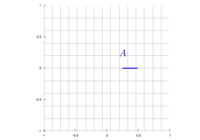
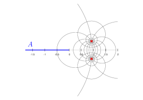
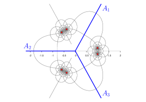
Figure 4: The cylinder $w$ with the cut $A$ is mapped via (27) to the center panel (we took $x=|u-v|/L=1/8$). The transformation (30) with $n=3$ has the effect shown in the right panel. The red crosses indicate the images $\zeta_{\infty}$, $\zeta^{\prime}_{\infty}$, $z_{k,3}$, $z^{\prime}_{k,3}$ of the points $w_{\infty}$, $w^{\prime}_{\infty}$.

Let us next compute the correlators appearing in equation (26) in the case where $A=(u,v)$. To this end we shall first introduce the complex coordinate $w=\sigma+i\tau$, which parametrizes an infinite cylinder of length $L$, i.e. $\sigma=\sigma+L$. The interval $A$ will be identified with the domain $u<w<v$. This cylinder can be mapped into the complex plane by the conformal transformation

$$\zeta=\frac{\sin\frac{\pi(w-u)}{L}}{\sin\frac{\pi(w-v)}{L}}$$ (27)

The points $w=u$ and $w=v$ are mapped into $\zeta=0$ and $\zeta=-\infty$ respectively, so that the interval $A$ corresponds to the negative real axis $\Re\,\zeta<0$. Moreover, the regions $\Im\,w\lessgtr 0$ are mapped into the regions $\Im\,\zeta\gtrless 0$. The points $(0,-\infty)$ and $(0,\infty)$, appearing in equation (26) correspond to the coordinates $w_{\infty}=-i\infty$ and $w^{\prime}_{\infty}=i\infty$, and, by equation (27), to the $\zeta$-coordinates (see fig 4)

$$w_{\infty}=-i\infty\Longrightarrow\zeta_{\infty}=e^{i\pi x},\qquad w^{\prime}_{\infty}=i\infty\Longrightarrow\zeta^{\prime}_{\infty}=e^{-i\pi x},\qquad x\equiv\frac{\ell}{L},\quad\ell=v-u$$ (28)

Notice that $x$ belong to the interval $(0,1)$ since $\ell\in(0,L)$. The Riemann surface ${\cal R}_{n}$ is constructed out by gluing cyclically $n$ copies of the complex $\zeta$-plane along the cut $A$. The uniforming parameter associated to ${\cal R}_{n}$ is given by

$$z=\zeta^{1/n}=\left(\frac{\sin\frac{\pi(w-u)}{L}}{\sin\frac{\pi(w-v)}{L}}\right)^{1/n}$$ (29)

Consequently, each of the points $\zeta_{\infty}$ and $\zeta^{\prime}_{\infty}$ give rises to $n$ points in the Riemann surface ${\cal R}_{n}$ with coordinates

$$z_{k,n}=e^{\frac{i\pi}{n}(x+2k)},\qquad z^{\prime}_{k,n}=e^{\frac{i\pi}{n}(-x+2k)},\qquad k=0,\dots,n-1$$ (30)

To compute (26) we first write it as

$$F^{(n)}_{\Upsilon}(A)\equiv F^{(n)}_{\Upsilon}(x)=\lim_{w\rightarrow-i\infty}\frac{\langle\prod_{k=0}^{n-1}\Upsilon_{k}(w,\bar{w})\,\Upsilon^{\dagger}_{k}(-w,-\bar{w})\rangle_{{\cal R}_{n}}}{\langle\Upsilon_{0}(w,\bar{w})\,\Upsilon^{\dagger}_{0}(-w,-\bar{w})\rangle_{{\cal R}_{1}}^{n}}$$ (31)

The $2n$ point correlator on ${\cal R}_{n}$, appearing in the numerator, can be transformed into a correlator on the complex $z$-plane by means on the conformal transformation of the primary field $\Upsilon$

$$\Upsilon(w,\bar{w})=\left(\frac{dz}{dw}\right)^{h}\left(\frac{d\bar{z}}{d\bar{w}}\right)^{\bar{h}}\Upsilon(z,\bar{z})$$ (32)

and a similar equation for $\Upsilon^{\dagger}$. From equation (29) one finds

$$\frac{dz}{dw}=\frac{z}{n}\frac{4\pi}{L}\sin(\pi x)\;(e^{\frac{i\pi}{L}(w-u)}-e^{-\frac{i\pi}{L}(w-u)})^{-1}(e^{\frac{i\pi}{L}(w-v)}-e^{-\frac{i\pi}{L}(w-v)})^{-1}$$ (33)

which in the limit $w\rightarrow\pm i\infty$ becomes

$$w\rightarrow-i\infty,\quad z \rightarrow z_{k,n}\Longrightarrow\frac{dz}{dw}\rightarrow\frac{z_{k,n}}{n}\;\Lambda$$ (34)

$$w\rightarrow i\infty,\quad z \rightarrow z^{\prime}_{k,n}\Longrightarrow\frac{dz}{dw}\rightarrow\frac{z^{\prime}_{k,n}}{n}\;\bar{\Lambda}$$ (35)

where

$$\Lambda=\frac{4\pi}{L}\sin(\pi x)e^{-2\pi|w|/L}e^{i\pi(u+v)/L}$$ (36)

In this limit the conformal transformation (32) yields

$$w\rightarrow-i\infty,\quad z \rightarrow z_{k,n}\Longrightarrow\Upsilon_{k}(w,\bar{w})\rightarrow\left(\frac{z_{k,n}}{n}\;\Lambda\right)^{h}\left(\frac{\bar{z}_{k,n}}{n}\;\bar{\Lambda}\right)^{\bar{h}}\,\Upsilon(z_{k,n},\bar{z}_{k,n})$$ (37)

$$w\rightarrow i\infty,\quad z \rightarrow z^{\prime}_{k,n}\Longrightarrow\Upsilon_{k}^{\dagger}(w,\bar{w})\rightarrow\left(\frac{z^{\prime}_{k,n}}{n}\;\Lambda\right)^{h}\left(\frac{\bar{z}^{\prime}_{k,n}}{n}\;\bar{\Lambda}\right)^{\bar{h}}\,\Upsilon^{\dagger}(z_{k,n},\bar{z}_{k,n})$$ (38)

Plugging these equations into (31), the factors proportional to $\Lambda$ and $\bar{\Lambda}$ cancel out and one is left with

$$F^{(n)}_{\Upsilon}(x)=n^{-2n(h+\bar{h})}\;\frac{\prod_{k=0}^{n-1}z_{k,n}^{h}\bar{z}^{\bar{h}}_{k,n}z_{k,n}^{\prime h}\bar{z}^{\prime\bar{h}}_{k,n}}{\left(z_{0,1}^{h}\bar{z}^{\bar{h}}_{0,1}z_{0,1}^{\prime h}\bar{z}^{\prime\bar{h}}_{0,1}\right)^{n}}\frac{\langle\prod_{k=0}^{n-1}\Upsilon(z_{k,n},\bar{z}_{k,n})\,\Upsilon^{\dagger}(z^{\prime}_{k,n},\bar{z}^{\prime}_{k,n})\rangle_{{\mathbb{C}}}}{\langle\Upsilon(z_{0,1},\bar{z}_{0,1})\,\Upsilon^{\dagger}(z^{\prime}_{0,1},\bar{z}^{\prime}_{0,1})\rangle_{{\mathbb{C}}}^{n}}$$ (39)

To simplify this expression, we can make a further conformal transformation from the complex plane to a cylinder of length $2\pi$,

$$z=e^{it}\rightarrow\Upsilon(t,\bar{t})=e^{i\pi(h-\bar{h})}z^{h}\,\bar{z}^{\bar{h}}\;\Upsilon(z,\bar{z})$$ (40)

which allow us to write (39) as

$$F^{(n)}_{\Upsilon}(x)=n^{-2n(h+\bar{h})}\;\frac{\langle\prod_{k=0}^{n-1}\Upsilon(t_{k,n},{t}_{k,n})\,\Upsilon^{\dagger}(t^{\prime}_{k,n},{t}^{\prime}_{k,n})\rangle_{\rm cy}}{\langle\Upsilon(t_{0,1},{t}_{0,1})\,\Upsilon^{\dagger}(t^{\prime}_{0,1},{t}^{\prime}_{0,1})\rangle_{\rm cy}^{n}}$$ (41)

where

$$t_{k,n}=\frac{\pi}{n}(x+2k),\qquad t^{\prime}_{k,n}=\frac{\pi}{n}(-x+2k),\qquad k=0,1,\dots,n-1$$ (42)

Since the latter parameters are all real we may as well write (39) in a compact form as

$$F^{(n)}_{\Upsilon}(x)=n^{-2n(h+\bar{h})}\;\frac{\langle\prod_{k=0}^{n-1}\Upsilon(\frac{\pi}{n}(x+2k))\,\Upsilon^{\dagger}(\frac{\pi}{n}(-x+2k))\rangle_{\rm cy}}{\langle\Upsilon(\pi x)\,\Upsilon^{\dagger}(-\pi x)\rangle_{\rm cy}^{n}}$$ (43)

where $\Upsilon(t)\equiv\Upsilon(t,t)$. After a shifting of the points in which the correlator is evaluated, this equation become (4), which was derived in reference Alcaraz et al. (2011) using the HLW approach. The function $F^{(n)}_{\Upsilon}(x)$ satisfies the following identities

$$F^{(n)}_{\Upsilon}(x)=\left(F^{(n)}_{\Upsilon}(x)\right)^{*}=F^{(n)}_{\Upsilon^{\dagger}}(x)=F^{(n)}_{\Upsilon}(1-x)$$ (44)

that can be derived from equation (39) using the transformation properties of correlators under inversion $z\rightarrow-1/z$ and rotations $z\rightarrow e^{i\alpha}z$. The last equality in (44) reflects the well know fact that the Rényi entropy $S_{n}(A)$ is the same as $S_{n}(B)$, where $B$ is the complement of $A$, which amounts to the replacement $\ell\rightarrow L-\ell$, that is $x\rightarrow 1-x$.

IV Bosonic theory: $XX$, $XXZ$ and excluded-$XXZ$ models

The first theory under study is a massless bosonic field $\varphi(z,\bar{z})$, with action:

$$\mathcal{A}[\varphi]=\frac{1}{8\pi}\int dz\,d\bar{z}\,\partial_{z}\varphi\,\partial_{\bar{z}}\varphi$$ (45)

This is a CFT with central charge $c=1$ and two types of primary fields. The first type is given by the vertex operators

$$V_{\alpha,\bar{\alpha}}\equiv\,:e^{i(\alpha\phi+\bar{\alpha}\bar{\phi})}:\,,$$ (46)

where $\phi$ , $\bar{\phi}$ are the chiral and anti-chiral parts of the bosonic field, solution of the equation of motion: $\varphi(z,\bar{z})=\phi(z)+\bar{\phi}(\bar{z})$. In the last equation $:\cdot:$ denotes normal ordering and $\alpha,\bar{\alpha}$ are real numbers. The vertex operator has conformal weights $(h,\bar{h})$=$(\alpha^{2}/2,\bar{\alpha}^{2}/2)$ Di Francesco et al. (1999):

$$\langle V_{\alpha_{1},\bar{\alpha}_{1}}(z_{1},\bar{z}_{1})\,V_{\alpha_{2},\bar{\alpha}_{2}}(z_{2},\bar{z}_{2})\rangle=(z_{1}-z_{2})^{\alpha_{1}\alpha_{2}}\,(\bar{z}_{1}-\bar{z}_{2})^{\bar{\alpha}_{1}\bar{\alpha}_{2}}$$ (47)

where $\langle\cdot\rangle$ denotes the correlator in the complex plane, and the neutrality condition implies that the correlator is different from zero only if $\alpha_{1}+\alpha_{2}=0$ and the same for the $\bar{\alpha}$’s. This result is indeed more general. Considering holomorphic fields $\bar{\alpha}=0$ only, one has ($z_{ij}\equiv z_{i}-z_{j}$):

$$\langle V_{\alpha_{1}}(z_{1})\dots V_{\alpha_{n}}(z_{n})\rangle=\prod_{i<j}[z_{ij}]^{\alpha_{i}\alpha_{j}}$$ (48)

if $\sum_{j}\alpha_{j}=0$, and zero otherwise. In a cylinder of length $2\pi$ parametrized by $w=-i\ln z$ this correlator is:

$$\langle V_{\alpha_{1}}(w_{1})\dots V_{\alpha_{n}}(w_{n})\rangle_{\rm{cy}}=\prod_{i<j}[2\sin(w_{ij}/2)]^{\alpha_{i}\alpha_{j}}$$ (49)

evaluating (49) in the points indicated in (4), i.e., in the set $\left\{2\pi j/n,2\pi(j+x)/n\right\}_{j},\,j=0,\dots,n-1$, one has :

$$F^{(n)}_{V_{\alpha}}(x)=\left(n^{-n}\left[\frac{\sin(\pi x)}{\sin(\pi x/n)}\right]^{n}\,\,\prod_{m=1}^{n-1}\left[\frac{\sin(\pi m/n)^{2}}{\sin{\frac{\pi(m-x)}{n}}\sin{\frac{\pi(m+x)}{n}}}\right]^{m-n}\right)^{\alpha^{2}}.$$ (50)

This function is constantly equal to one:

$$F^{(n)}_{V_{\alpha}}(x)=1\qquad\forall n,\alpha,$$ (51)

a fact that can be proved by comparing the zeroes in $x$ of the numerator and in the denominator of (50). There are zeroes of order $n$ in $x\in\mathbb{Z}$ in both the numerator and the denominator. As analytic functions, this implies they are proportional, the proportionality constant being 1 as can be immediately seen in the $x\to 0$ limit. We thus observe that the entropy of excitations corresponding to vertex operators coincide with the ground state entropy according to the CFT prediction (4).
Let us now focus our attention in the other primary field in the theory: $i\partial\phi$, with conformal weights $(h,\bar{h})=(1,0)$. We will use the correlators of $i\partial\phi$ in the plane:

$$-\langle\partial\phi(z_{1})\partial\phi(z_{2})\rangle=\frac{1}{{z_{12}}^{2}}$$ (52)

and the Wick theorem:

$$\langle\prod_{j=0}^{2n}i\partial\phi(z_{j})\rangle=\mbox{Hf}\,\left[\frac{1}{{z_{ij}}^{2}}\right]_{1\leq i,j,\leq 2n}$$ (53)

where Hf [ ] denotes the Haffnian ($S_{2n}$ is the permutation group of the $2n$ indexes):

$$\mbox{Hf}\,(A)=\frac{1}{2^{n}n!}\sum_{\pi\in S_{2n}}\prod_{i=1}^{n}\,A_{\pi(2i-1),\pi(2i)},$$ (54)

and where the matrix in (53) has a null diagonal. This matrix being dependent only on $i-j$, can actually be written as a determinant Di Francesco et al. (1999):

$$\mbox{Hf}\,\left[\frac{1}{{z_{ij}}^{2}}\right]=\mbox{det}\,\left[\frac{1}{z_{ij}}\right].$$ (55)

In the cylinder $w=-i\ln z$, and taking again the $2n$ coordinates $w_{j}$ as in (4) one gets:

$$F^{(n)}_{i\partial\phi}(x)=n^{-2n}\left[\sin{\pi x}\right]^{2n}\,\mbox{det}\,\left[\frac{1}{\sin{(w_{ij}/2)}}\right]_{1\leq i,j\leq 2n},$$ (56)

The $n=2,3$ values of (56) are reported:

$$F^{(2)}_{\Upsilon_{1}}(x)=1-2\mathbf{r}^{2}+3\mathbf{r}^{4}-2\mathbf{r}^{6}+\mathbf{r}^{8}$$ (57)

$$F^{(3)}_{\Upsilon_{1}}(x)=\frac{1}{729}\left[1-4\mathbf{s}+\frac{2\mathbf{s}^{3}}{\mathbf{s}_{+}}-\frac{2\mathbf{s}^{3}}{\mathbf{s}_{-}}+\frac{3\mathbf{s}^{2}}{\mathbf{s}_{+}\mathbf{s}_{-}}-\frac{\mathbf{s}^{3}}{\mathbf{s}_{+}^{3}}+\frac{\mathbf{s}^{3}}{\mathbf{s}_{-}^{3}}\right]^{2}$$ (58)

where $\mathbf{r}\equiv\sin\pi x/2$, $\mathbf{s}\equiv\sin{\pi x/3}$, $\mathbf{s}_{\pm}\equiv\sin{\pi(1\pm x)/3}$. These values will be compared below with the numerical values of $F^{(n)}$ obtained for the finite-size states $|i\partial\phi\rangle$ in the lattice models described by the bosonic theory.

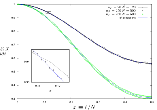
Figure 5: Rényi entropy ratio of the particle-hole excitation in the $XX$/free fermion model, $n=2,3$, and two different sizes, vs. the CFT prediction equations (57, 58) (continuous lines). For $n=2$, a system with filling fraction 1/6 is also shown. The inset is a zoom of the region defined by the small rectangle over the data-set in the body of the figure.

Figure 6: $F^{(2,3)}_{|\partial\phi|^{2}}$ for a right-left particle-hole excitation in the $XX$ model with $N=120$ sites. Two values of the external field $J$ are shown: for $J=0$ and $J=1/2$ the filling fractions are $1/2$ and $1/3$ respectively. Continuous lines (indistinguishable from the numerical data for $n=2$) are the CFT prediction.

IV.1 $XX$ model

As explained in the appendix, the $XX$ model is mapped into the lattice fermion problem (6). In the continuum limit, this becomes a massless Dirac fermion whose low-energy regime is exactly formulated, via the bosonization procedure, as a free bosonic theory (45). According to this map, $e^{i\phi}$ ($e^{-i\phi}$) corresponds in the fermionic language to the creation of a fermion (hole) (c.f. table 1).
Let us illustrate the law $F^{(n)}_{V_{\alpha,\bar{\alpha}}}(x)=1$ for three different states of the finite-size $XX$ problem. Consider $|V_{\alpha,\bar{\alpha}}\rangle$ with $(\alpha,\bar{\alpha})=$ (1,-1). It is the Umklapp excitation (c.f. table 1) which, as said in section II, presents a vanishing excess of entropy. The same applies for the state $(\alpha,\bar{\alpha})=$ (-1,0), which corresponds to the $(a)$ excitation; to $(\alpha,\bar{\alpha})=$ (1,1) which corresponds to the $(b)$ state (c.f. figure 1), and, in general, to all the low-energy compact excitations.
We now focus in the state $|i\partial\phi\rangle$ with total momentum $P=2\pi/N$. In the $XX$/free fermion model it corresponds to the particle-hole excitation (c.f. table 1). In figure 5 we present the quantity $F^{(2,3)}_{i\partial\phi}$ for lattices with different sites and filling fractions, together with the CFT predictions (57), (58). A further prediction is shown in figure 6 for the excitation $\partial\phi\bar{\partial}\bar{\phi}$, which corresponds in the lattice to a particle-hole excitation on the top of both the right and left Fermi points (c.f. table 1). The quantity $F^{(2,3)}_{\partial\phi\bar{\partial}\bar{\phi}}$ is compared with the CFT prediction, which is the square of (57,58). We observe a very good agreement.
Finally, in reference Alcaraz et al. (2011) it was shown how, in the $x<<1$, $n\to 1$ limits, (4) results in the law (10), which was tested in the $XX$ model in figure 2. Interestingly enough, and as can be seen in the figure, the law (10) works also for non-primary states.

IV.2 $XXZ$ and excluded-$XX$ models

We define the $XXZ$ spin chain:

$$H_{XXZ}=-\frac{1}{2}\sum_{j=1}^{N}\left[\sigma_{j}^{x}\sigma_{j+1}^{x}+\sigma_{j}^{y}\sigma_{j+1}^{y}+\Delta\sigma_{j}^{z}\sigma_{j+1}^{z}\right],$$ (59)

where PBCs are assumed (for $\Delta=0$ one gets the $XX$ model). This model is integrable Yang and Yang (1966) and gapless for $-1\leq\Delta<1$. In the continuum limit it is described by the aforementioned bosonic CFT compactified in a circle of radius $K=\pi/(2\cos^{-1}(\Delta))$. We had access to the exact entanglement entropy of this model through its exact diagonalization.
We first consider the vertex states $|V_{\alpha}\rangle$ in the $XXZ$ model. The studied excitations were the following: the $(a)$ and $(b)$-types defined in table 1, the Umklapp state and the states $|V_{\alpha}\rangle$ with $\alpha=1,2,3$ (c.f. Alcaraz et al. (2011)). We had access to the exact wave-function of the desired states (and hence to the entropy) through exact diagonalization. We verified that, as predicted by CFT, the $n$-Rény entropy coincides (up to oscillations) with the ground state entropy for $n=2,3$, in systems with several critical values of $\Delta$, filling fractions and sizes up to $N=30$ sites.
Secondly, we studied the state $|i\partial\phi\rangle$ which is the lowest energy one in the sector with total momentum $P=2\pi/N$. The function $F^{(2,3)}$ is compared with the CFT prediction in figure 7-(a).

The excluded-$XXZ$ model Alcaraz and Bariev (1999b, a) is an exactly integrable extension of the standard $XXZ$ chain. In this model the up spins ($\sigma^{z}$-basis) have an effective size $t+1$ ($t=0,1,2,\ldots$) in units of lattice spacing, which means that up spins are not allowed at distances smaller than $t+1$ sites. The model is defined by the Hamiltonian

$$H=-\frac{1}{2}\sum_{j=1}P_{t}(\sigma_{j}^{z}\sigma_{j+1}^{z}+\sigma_{j}^{y}\sigma_{j+1}^{y}+\Delta\sigma_{j}^{z}\sigma_{j+1}^{z})P_{t},$$ (60)

where $\Delta$ is the anisotropy and $P_{t}$ projects out states in which pairs of up spins are at distance smaller than $t+1$ sites. For $t=0$ one recovers the standard $XXZ$ model (59) where we only exclude up spins at the same site. Like the $XXZ$ model there is a $U(1)$ symmetry, due to the conservation of the number of up spins. The model is critical for $-1\leq\Delta<1$, and is ruled by a Luttinger liquid CFT ($c=1$) whose Luttinger parameter $K$ depends on the value of $t,\Delta$ and the density of up spins. For $\Delta=0$, i. e., the excluded $XX$ chain Alcaraz and Bariev (1999a) $K$ is known analytically, namely $K=(1-t\rho)^{2}$ where $\rho$ is density of up spins ($0\leq\rho\leq\frac{1}{1+t}$).
For $t=1,2$ and $\Delta=0$ we find similar results as for the $XXZ$ model. Figure 7-(b) shows some numerical results for the vertex and the particle-hole excitation.

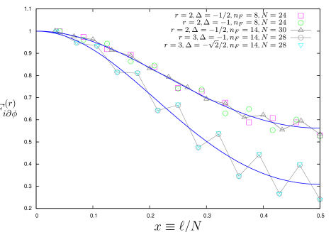
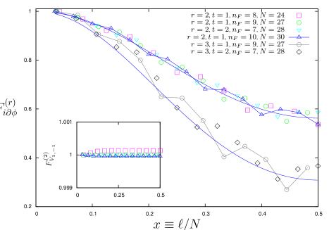
(a)	(b)

Figure 7: Entropy ratio $F^{(r)}_{i\partial\phi}$, $r=2,3$, for the particle-hole state of the $XXZ$ model for different sizes and values of the anisotropy $\Delta$ in the critical region (left) and for the excluded-$XX$ model for $t=1,2$ and several filling fractions (right). On inset the Umklapp excitation is studied instead, which confirms the law (51).

IV.3 Universality of Rényi entropy oscillations

Specially important are the models described by Luttinger Liquid field theories, which are CFTs with central charge equal to one. Their ground states obey hence the law (2) for the Rényi entropy with $c=1$. On the other hand, finite-size ground states of these models were shown in reference Calabrese et al. (2010) to obey (2) up to some oscillations whose amplitude turns out to be related to the Luttinger Liquid parameter which depends on the microscopic couplings of the Hamiltonian. In this subsection we investigate the oscillations of some elementary excitations of the $XX$ and $XXZ$ models.
For the ground state, the deviation with respect to the CFT prediction (2), $S_{n}^{\rm{CFT}}$, takes the universal form Calabrese et al. (2010); Xavier and Alcaraz (2011); Cardy and Calabrese (2010):

$$S_{n}(\ell)-S_{n}^{\rm{CFT}}(\ell)=f_{n}\,\mathcal{F}_{n}(\ell/N)\,\cos(2k_{F}\ell)\,|D(\ell,N)\sin k_{F}|^{p(n,K)},$$ (61)

where $k_{F}$ the Fermi momentum, $D(\ell,N)=\frac{N}{\pi}\sin{\pi\ell/N}$ is the chord distance, $f_{n}$ is a non-universal constant and $\mathcal{F}_{n}$ is a universal function depending in general on the parity of $N$. The exponent $p(n,K)=-2K/n$ is a function of the Rényi index and of the Luttinger Liquid parameter, $K$. In the models studied in Calabrese et al. (2010); Xavier and Alcaraz (2011); Cardy and Calabrese (2010), no oscillations are found for the von Neumann entropy (i.e. for $n=1$ in (61)). We also observe this fact for all the excitations considered in this article. In the present section we will provide numerical evidence that the same behaviour (61) holds for low-energy excitations, the function $\mathcal{F}_{n}$ depends in a universal way on the given excitation and the exponent $p(n,K)$ is given by $-2K/n$, at least for some of the excitations considered.

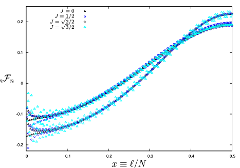
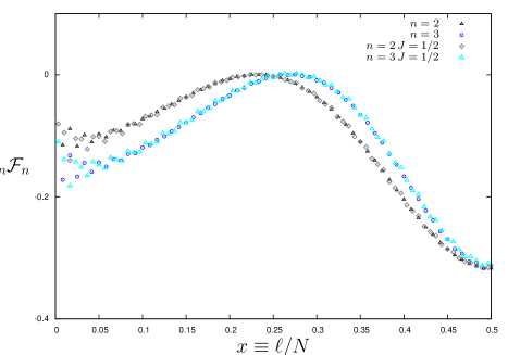
(a)	(b)

Figure 8: (a) Function $f_{n}\,\mathcal{F}_{n}$ corresponding to the particle-hole excitation of the $XX$ model with four different values of the field $J$. $n=2,3$ cases are shown (the former being the upper curve at the half of the chain). (b) idem for the right-left particle-hole excitation. Colors are as in figure 6.

For the $XX$ in an external $z$-field of strength $J$ (c.f. equation (75), $\gamma=0$), the law (61) holds for all the excitations considered. For this model $K=1$ regardless the value of $J$. The $N$-dependence of $S_{n}-S_{n}^{\rm{CFT}}$ at half of the chain shows a power law behaviour compatible with $p(n,1)=-2/n$ for $n=2,3$. Further numerical evidence can be found in figure 8 for the non-chiral and chiral particle-hole excitations: the same function $f_{n}\mathcal{F}_{n}$ can be found for common excitations in systems with different values of $J$ and filling fractions, showing the validity of equation (61) for $K=1$, the function $\mathcal{F}_{n}$ depending only on the excitation, and with $p(n,1)=-2/n$ for $n=2,3$.

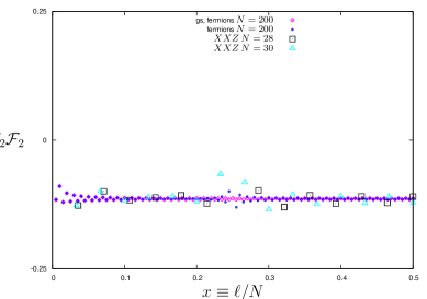
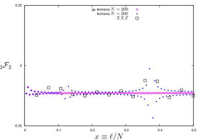
(a)	(b)

Figure 9: Functions $f_{n}\,\mathcal{F}_{n}$ describing the amplitude of the Rényi oscillations for several excitations in the $XX$ and $XXZ$ ($\Delta=-1/2$) models with $N=240,500$ and $28$ respectively. (a) and (b) correspond to the ($a$) and ($b$) excitations defined in table 1. The universality of $\mathcal{F}_{n}$ is apparent, being this function equal with the ground state case, which is shown for comparison.

On the other hand, for vertex excitations one observes the validity of the scaling (61) with $p(n,K)$ also for $K\neq 1$. A first illustration of this fact can be found in the Umklapp excitation: as mentioned before, the state $|V_{1,-1}\rangle$ of the $XX$ model has exactly the same Rényi entropy as the ground state in the lattice. Moreover, the same state in the $XXZ$ model exhibits the same entropy of the ground state up to corrections of the order of $10^{-3}$ (i.e., the same oscillations) for systems with 30 sites Alcaraz et al. (2011) (see also figure 7-(a)). This implies that, for both $XX$ and $XXZ$ models, $\mathcal{F}_{n}$ is common to the ground state and the $|V_{1,-1}\rangle$ state. Further numerical evidence is shown in figure 9-a,b, where the ($a$) and ($b$) states in the $XX$ case are compared with the $XXZ$ case with $\Delta=-1/2$. The function $\mathcal{F}_{n}$ for vertex excitations turns out to be the same as for the ground state (apparently a constant function, c.f. figure 9, in agreement with Calabrese et al. (2010)). We obtain analog results for other values of $\Delta$ and for $n=3$, with $p(n,K)=-2K/n$ as in (61). The case of the particle-hole excitation for $\Delta\neq 0$ is more controversial up to the sizes we have investigated, and will be studied in a future work which is in preparation Ibáñez Berganza (2011).

V Fermionic theory and entanglement in the critical Ising model

The second CFT we examine is the critical Ising model, whose action is given by

$$\mathcal{A}[\psi]=\frac{1}{8\pi}\,\int dz\,d\bar{z}\,\left[\psi\partial_{\bar{z}}\psi+\bar{\psi}\partial_{z}\bar{\psi}\right]$$ (62)

where $\psi$ is a free Majorana fermion. The solution to the equations of motion being $\psi(z,\bar{z})=\psi(z)+\bar{\psi}(\bar{z})$. This theory is conformal, with $c=1/2$ and with primary operators $\sigma$ and $\psi$ having the conformal weights:

$$(h,\bar{h})_{\sigma}=(\frac{1}{16},\frac{1}{16}),\qquad(h,\bar{h})_{\psi}=(\frac{1}{2},0).$$ (63)

Let us first study the function $F^{(n)}_{\sigma}$. One can compute Di Francesco et al. (1999) the correlators of the field $\sigma$ by bosonization. Two Majorana fermions (labelled 1 and 2) can be combined into a Dirac Fermion $\Psi(z)=2^{-1/2}(\psi_{1}(z)+i\psi_{2}(z))$. $\Psi$ is in this way a (1/2,0) primary field with two-point correlator:

$$\langle\Psi(z_{1})^{\dagger}\Psi(z_{2})\rangle=\langle\psi(z_{1})\psi(z_{2})\rangle=\frac{1}{z_{12}}.$$ (64)

The CFT describing the Dirac fermion has as central charge twice the Majorana fermion central charge, i.e., $c=1$. The Dirac theory can be mapped into a free bosonic theory with action (45) in such a way that the spectrum of both theories coincide and that to each operator in the Dirac theory there corresponds an operator in the bosonic theory with common algebra and correlators. For the field $\Psi$, this mapping is:

$$\Psi(z)=e^{i\phi(z)},\qquad\bar{\Psi}(\bar{z})=e^{i\bar{\phi}(\bar{z})}$$

and for $\sigma$ (as can be checked from the matching of the conformal weights):

$$\sigma_{1}(z,\bar{z})\sigma_{2}(z,\bar{z})=2^{1/2}\cos(\varphi(z,\bar{z})/2).$$

As described in Di Francesco et al. (1999), the following trick is used for the computation of a chain of $\sigma$ correlators. Two copies of $\sigma$ operator chains are constructed

$$\langle\sigma_{1}(z,\bar{z})\sigma_{2}(z,\bar{z})\sigma_{1}(w,\bar{w})\sigma_{2}(w,\bar{w})\rangle=\langle\sigma(z,\bar{z})\sigma(w,\bar{w})\rangle^{2}=2\left<\cos\frac{\varphi(z,\bar{z})}{2}\,\cos\frac{\varphi(w,\bar{w})}{2}\right>.$$

Using the vertex operator correlator (48) one arrives to:

$$\langle\sigma(z,\bar{z})\sigma(w,\bar{w})\rangle^{2}=|z-w|^{-1/2},$$

and, for a set of $2n$ fields, to:

$$\langle\sigma(z_{1}\bar{z}_{1})\dots\sigma(z_{2n}\bar{z}_{2n})\rangle^{2}=2^{-n}\sum_{\{\alpha_{j}=\pm 1\}}\,\prod_{i<j}|z_{i}-z_{j}|^{\alpha_{i}\alpha_{j}/2}$$

where the sum is subject to: $\sum_{j}\alpha_{j}=0$. In the cylinder $w=-i\ln z$ this is:

$$\langle\sigma(w_{1}\bar{w}_{1})\dots\sigma(w_{2n}\bar{w}_{2n})\rangle^{2}=2^{-n}\sum_{\{\alpha_{j}=\pm 1\}}\,\prod_{i<j}|\sin w_{ij}|^{\alpha_{i}\alpha_{j}/2}$$ (65)

With this information one can construct the function $F^{(n)}_{\sigma}$, which reads:

$$\left[F^{(n)}_{\sigma}(x)\right]^{2}=|\sin(\pi\,x)|^{n/2}\sum_{\{\alpha_{j}=\pm 1\}}\left[\prod_{q=0}^{n-1}\,\prod_{j=1}^{n-q}\left|\sin\frac{\pi(q+x)}{n}\right|^{\frac{\alpha_{2j-1}\alpha_{2(j+q)}}{2}}\right.$$

$$\left.\prod_{q=1}^{n-1}\,\prod_{j=1}^{n-q}\left|\sin\frac{\pi(q-x)}{n}\right|^{\frac{\alpha_{2j}\alpha_{2(j+q)-1}}{2}}\left|\sin\frac{\pi q}{n}\right|^{\frac{\alpha_{2j}\alpha_{2(j+q)}}{2}}\right]\,=1.$$ (66)

This function can be proved to be constantly equal to one for all values of $n$, in the same way that this fact was proved for $F^{(n)}_{V_{\alpha}}$. The square of equation (66) can be written as the product of two terms: the function $|\sin(\pi\,x)|^{n}$ on the one hand, which presents a zero of order $n$ for each $x\in\mathbb{Z}$, and the sum on the permutations squared, which presents poles in $x\in\mathbb{Z}$ of order $n$. Indeed, for each integer whose rest of the division by $n$ is $p>0$, there is a pole of order $n-p$ in the $q=p$ product in the second line of (66), and a pole of order $p$ in the $q=n-p$ product in the first line, and this happens since, for a given $p$, the permutation $\{\alpha_{j}=(-1)^{j}\}$ satisfies $\sum_{j=1}^{n-p}\alpha_{2j}\alpha_{2(j+p)-1}=n-p$ and $\sum_{j=1}^{p}\alpha_{2j-1}\alpha_{2(j+n-p)}=p$. We hence find the CFT prediction that the entropy of $\sigma$ excitations coincides again with the ground state entropy.
We repeat the game for the thermal field $\varepsilon(z,\bar{z})\equiv i\psi(z)\bar{\psi}(\bar{z})$, with conformal weights $\left(h,\bar{h}\right)=\left(\frac{1}{2},\frac{1}{2}\right)$. For the computation of $F^{(n)}_{\varepsilon}$ we use the $2n$-point correlator of $\varepsilon$’s (cf. Di Francesco et al. (1999), p. 444), which can be inferred from the $\psi$ correlator (64):

$$\langle\varepsilon(z_{1},\bar{z}_{1})\dots\varepsilon(z_{2n},\bar{z}_{2n})\rangle=$$

$$\langle\psi(z_{1})\dots\psi(z_{2n})\rangle\langle\bar{\psi}(\bar{z}_{1})\dots\bar{\psi}(\bar{z}_{2n})\rangle=\left|\mbox{Pf}\,\left[\frac{1}{z_{ij}}\right]_{1\leq i,j\leq 2n}\right|^{2},$$ (67)

where Pf means the Pfaffian:

$$\mbox{Pf}\,(A)=\frac{1}{2^{n}n!}\sum_{\pi\in S_{2n}}\mbox{sign}(\pi)\prod_{i=1}^{n}\,A_{\pi(2i-1),\pi(2i)}.$$ (68)

In the cylinder $w=-i\ln z$ and taking the $2n$ coordinates $w_{ij}$ as in (4), one arrives to:

$$\langle\prod_{j=1}^{2n}\varepsilon(w_{j},\bar{w}_{j})\rangle=\left(\mbox{Pf}\,\left[\frac{1}{\sin{(w_{ij}/2)}}\right]_{1\leq i,j\leq 2n}\right)^{2}$$ (69)

and using that the Pfaffian of an antisymmetric matrix is the square root of its determinant, one finds that $F^{(n)}_{\varepsilon}(x)$ coincides with the value computed in section IV for the field $i\partial\phi$ (c.f. equation (56)):

$$F^{(n)}_{\varepsilon}(x)=F^{(n)}_{i\partial\phi}(x).$$ (70)

Finally, using (67), one obtains:

$$F^{(n)}_{\psi}(x)=\sqrt{F^{(n)}_{i\partial\phi}(x)}.$$ (71)

V.1 Ising model on the lattice

Consider the critical Ising model on a transverse field (ITF)

$$H_{I}=-\frac{1}{2}\sum_{j=1}^{N}\,\left(\sigma_{j}^{x}\sigma_{j+1}^{x}+J\,\sigma_{j}^{z}\right).$$ (72)

The model is integrable and critical for $J=1$. The critical model is described in the continuum limit by the free Majorana fermion (62) Di Francesco et al. (1999), as can be seen from the spectra of its free-fermionic formulation (85). We identified the states $|\sigma\rangle$, $|\varepsilon\rangle$, $|\psi\rangle$ in the finite size Ising model through their finite-size scaling of energy and momentum and for these states we computed the entanglement entropies and the quantity $F^{(n)}$ via the method described in Chung and Peschel (2001) and in the appendix.

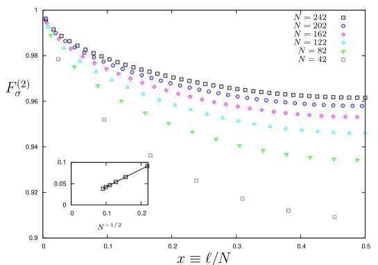
Figure 10: The function $F^{(2)}_{\sigma}$ seems to converge to the CFT prediction $F^{(n)}_{\sigma}(x)=1$ in the large $N$-limit of the critical Ising model. The inset shows the $N^{-1/2}$-dependence of $F^{(2)}(1/2)$.

The excitation $|\sigma\rangle$ corresponds in the lattice to the lowest energy state in the parity -1 sector. Figure 10 shows the quantity $F^{(2)}_{\sigma}$ for systems of several sizes up to $N=242$. One observes that, although the $N$-scaling is slower than in the bosonic case, the curve seems to converge to the CFT prediction (66) for large $N$ (see $N$ scaling of $F_{\sigma}^{(2)}(1/2)$ in the inset). For $F^{(3)}_{\sigma}$ we obtain analog results.

On the other hand, a comparison between the numerical values for the quantities $F^{(n)}_{\psi}$, $F^{(n)}_{\varepsilon}$, $n=2,3$ and the laws (70,71) is shown in figure 11. Once more, the agreement between CFT and finite-site lattices is remarkable.

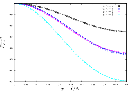
Figure 11: $n=2$ and 3-Rényi entropy ratio for the states $|\psi\rangle$, $|\varepsilon\rangle$ of a $N=200$ critical Ising, compared with the CFT predictions for these fields (continuous curves).

VI Descendant fields

The results presented so far give a strong numerical support to the validity of equation (43) for the entropy ratio $F^{(n)}_{\Upsilon}$ when $\Upsilon$ is a primary field. A natural question is whether that formula also applies when $\Upsilon$ is not a primary field but a descendant. We have not yet found a definite answer to this question but there are some observations that may eventually lead to a solution (for details see Ibáñez Berganza (2011)). Let us first recall that in the field theory construction of the reduced density matrix, $\rho_{\Upsilon}$, one inserts into the path integral an operator at $\tau=-\infty$, and another one at $\tau=\infty$, in order to create the incoming and outgoing states associated to $\Upsilon$ and $\Upsilon^{\dagger}$. These operators are inserted in a cylindrical geometry and hence the corresponding operators must be the conformal transformed of those defined on the complex plane. For primary fields, the latter conformal transformation is rather simple but for descendant fields it generates additional fields in the conformal tower. A typical example is the energy-momentum tensor, $T$, whose conformal transformation, from the complex plane to the cylinder, involves a constant term proportional to the Schwarzian derivative. Hence in this case the operators to be inserted at $\tau=\pm\infty$ involve $T$ plus a constant term. However this constant term cancels out in the conformal transformation (29) from the cylinder to the uniformizing plane $z$, so that the final expression for $F^{(n)}_{T}$ is given by equation (39) with $\Upsilon$ replaced by $T$ in the $2n$-point correlator on the complex plane. The same result can be obtained for the descendant field $\partial^{2}\phi$ of the $c=1$ theory, and we expect this result to hold in general. It would thus seem that equation (39) must also be valid for descendant fields. However the numerical results give only a partial confirmation of this conjecture, which we now explain in more detail.
Let us first consider the entropy of descendant fields in the sector with $(h,\bar{h})=(2,0)$ of the bosonic CFT. This space is the first (two-dimensional) degenerated sector of the identity tower in the bosonic CFT, and it is expanded by the fields $:(\partial\varphi)^{2}:$ and $:\partial^{2}\varphi:$ (the former being proportional to the stress-energy tensor of the theory, $T$). In the $XX$ and $XXZ$ models this sector has total energy and momentum $E=P=4\pi/N$.
In reference Alcaraz et al. (2011) it was noticed that the entropy of degenerate sectors could depend on the particular state in the sector. We will provide a example of this fact. Let $|1\rangle$, $|2\rangle$ denote a basis of the $(h,\bar{h})=(2,0)$ sector in a finite-size realization of the $XX$ chain. We computed the entropy $S_{2}$ for a general eigenvector of the $XX$ model in the mentioned sector:

$$|v\rangle=\cos\alpha|1\rangle+e^{i\beta}\sin\alpha|2\rangle$$ (73)

via exact diagonalization. Figure 12 shows $F^{(2)}_{|v\rangle}$ for several values of $\alpha$ and $\beta$, together with the entropy of the state $(1:2)$ computed with the correlation matrix method exposed in the appendix (circles). The states $(1:2)$ and $(2:1)$ constitute a basis of the sector, an both have the same entropy. Different grey levels in fig.12 denote different values of $\alpha$. There is a certain linear combination $|v\rangle$ for which the entropy coincides with the entropy of the state $(1:2)$, which turns out to have the lowest value. The CFT prediction for $T$, obtained using equation (39), is also reported in figure 12 and it seems to coincide with one of the states $|v\rangle$.
As another example, let us consider the descendant state $(1:2)$, whose field theory counterpart must be a linear combination $Y$ of the operators

$$Y=\cos\alpha\,\,\partial^{2}\phi+e^{i\beta}\sin\alpha\,\,T$$ (74)

The values of $\alpha$ and $\beta$ can be chosen to fit the numerical values of $F^{(2)}_{(1:2)}$ to the value of $F^{(2)}_{Y}$ obtained using equation (39). The result shown in fig 13, shows a remarkable agreement, which however is not as good as in the case of primary fields. Another example is the entropy of the energy-momentum tensor of the Ising model, where the CFT prediction given by equation (39) disagrees strongly with the numerical results. All this shows that the general application of this formula for descendants fields deserves further clarification.

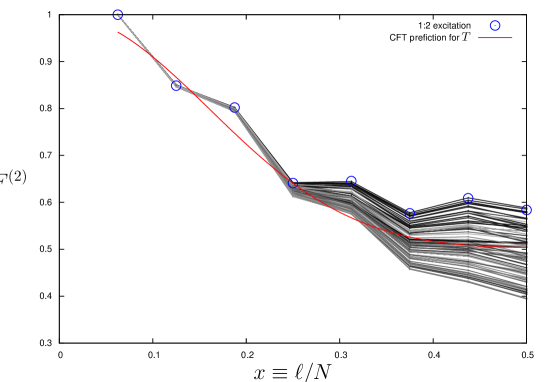
Figure 12: $n=2$ entropy ratio of several states in the $(h,\bar{h})=(2,0)$ sector of the $XX$ model with $N=16$.

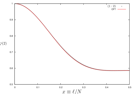
Figure 13: $n=2$ entropy ratio corresponding to the $(1:2)$ excitation of the $XX$ model with $N=400$ (points). The continuous curve is the a fit with the function $F^{(2)}_{Y}$ with $Y$ given by (74).

VII Conclusions and perspectives

The main findings reported in this article are summarized in what follows. The universality of the ground state Rényi entropy of entanglement at criticality is generalized to low-energy excitations represented by primary fields in CFT, as stated in reference Alcaraz et al. (2011), the $n$-th Rényi entropy being related to the $2n$-point correlator of the corresponding field. In this work, this result is derived in the more general framework of the Calabrese and Cardy article of 2004. The result is found to reproduce correctly the entropy of primary states of several models: the $XX$, $XXZ$ and excluded-$XXZ$ models in the $c=1$ universality class, and the Ising model in the $c=1/2$ universality class. Predictions for the low-$\ell$ behaviour of the von Neumann entropy are also numerically verified for bosons. We present numerical evidence of the universality of the parity effect of the Rényi entropy also for excited states, although further investigation is needed.
Finally, we have studied the Rényi entropies of some descendant states in the $XX$ and the Ising model, finding a partial sucess of the analytic approach which indicates that further investigation is required to fully understand the entropies of all the low energy states in critical lattice systems.

VIII Acknowledgements

This work was supported by the Spanish projects FIS2009-11654 and QuiteMad. We acknowledge the IFT (UAM/CSIC) for letting us use the high-performance computing cluster Hydra.

Appendix A Entanglement in the $XY$ model via correlation matrices

We consider the $XY$ model for $N$ spin-1/2 particles with periodic boundary conditions (PBC) in an external $z$ field.

$$H_{XY}=\frac{-1}{2}\sum_{j=1}^{N}\frac{1}{2}\left[(1+\gamma)\sigma^{x}_{j}\sigma^{x}_{j+1}+(1-\gamma)\sigma^{y}_{j}\sigma^{y}_{j+1}\right]+J\sigma_{j}^{z}$$ (75)

where $\sigma^{\alpha}$ are the Pauli matrices:

$$\sigma^{x}=\left(\begin{array}[]{cc}0&1\\ 1&0\end{array}\right),\qquad\sigma^{y}=\left(\begin{array}[]{cc}0&-i\\ i&0\end{array}\right),\qquad\sigma^{z}=\left(\begin{array}[]{cc}1&0\\ 0&-1\end{array}\right)$$

This generalizes the Ising (ITF) ($\gamma=1$) and $XX$ ($\gamma=0$, $J=0$) models. Defining the raising and lowering spin operators $\sigma^{\pm}=\frac{1}{2}(\sigma^{x}\pm i\sigma^{y})$ we have:

$$H_{XY}=\frac{-1}{2}\sum_{j=1}^{N}\,\left[\sigma^{+}_{j}\sigma^{-}_{j+1}+\gamma\,\sigma^{+}_{j}\sigma^{+}_{j+1}+\mbox{h.c.}\right]+J\sigma_{j}^{z}$$

A Jordan-Wigner transformation is now performed to express (75) in terms of true fermions $\{c_{m}^{\dagger},c_{n}\}=\delta_{m,n}$. They are defined as:

$$c_{m}=\left(\prod_{j<m}\sigma^{z}_{j}\right)\,\sigma_{m}^{-}$$ (76)

and they satisfy

$$c^{\dagger}_{N}c_{1}=-(-1)^{n_{\downarrow}}\sigma^{+}_{N}\sigma_{1}^{-}$$ (77)

where $n_{\downarrow}\equiv N-n_{F}$ is the number of down spins and

$$n_{F}=\sum_{j=1}^{N}\frac{s_{j}^{z}+1}{2}$$ (78)

is the number of up spins ($s_{j}^{z}$ being the eignevalue of $\sigma_{j}^{z}$) and also the number of fermions. Equation (77) determines the boundary conditions in the fermionic formulation of (75) and the Hamiltonian reads ($c_{N+1}=(-1)^{n_{\downarrow}}c_{1}$):

$$H_{XY}=\frac{1}{2}\sum_{j=1}^{N}\,\left[c^{\dagger}_{j}c_{j+1}+\gamma\,c^{\dagger}_{j}c^{\dagger}_{j+1}+\mbox{h.c.}\right]-2Jc^{\dagger}_{j}c_{j}$$

A Fourier transform is now performed. The $N$ fermionic modes, $\{d_{j}^{\dagger},d_{j^{\prime}}\}=\delta_{j,j^{\prime}}$ are defined:

$$d_{j}=\frac{1}{\sqrt{N}}\sum_{m=1}^{N}e^{-2ik_{j}m}\,c_{m},$$ (79)

(where $k_{j}\equiv 2\pi j/N$ is the momentum associated with index $j$), in such a way that:

$$H_{XY}=\sum_{j\in\Omega}\,A_{j}\,d_{j}^{\dagger}\,d_{j}+iB_{j}\,\left[d_{j}^{\dagger}d_{-j}^{\dagger}+d_{j}d_{-j}\right].$$ (80)

where we defined $A_{j}$, $B_{j}$ :

$$A_{j}=\cos{k_{j}}-J,\qquad B_{j}=\frac{\gamma}{2}\sin{k_{j}},$$ (81)

and where the set of momentum indexes $\Omega$ is such that the resulting allowed momenta $k_{j}$, $j\in\Omega$, are those specified later in equation A. The Hamiltonian (80) describes interacting fermions and can be diagonalized throught a Bogolubov transformation. Defining the fermionic modes ($u_{j}^{2}+v_{j}^{2}=1$):

$$b_{j}^{\dagger}=u_{j}\,d_{j}^{\dagger}+iv_{j}\,d_{-j}$$

$$b_{-j}=u_{j}\,d_{-j}+iv_{j}\,d_{j}^{\dagger},$$ (82)

and imposing that the Hamiltonian for the $j$, $-j$ modes has the diagonal form $(E_{j}\,b_{j}^{\dagger}b_{j}-E_{j}\,b_{j}b_{j}^{\dagger})/2$, i.e., that:

$$H_{XY}=\frac{1}{2}\sum_{j}\,E_{j}\,b_{j}^{\dagger}b_{j}-E_{j}\,b_{j}b_{j}^{\dagger}=\sum_{j}\,E_{j}\,b_{j}^{\dagger}b_{j}-\frac{1}{2}E_{j}$$ (83)

we obtain the Bogolubov equations to be satisfied by $u_{j}$, $v_{j}$:

$$u_{j}^{2}-v_{j}^{2}=A_{j}/E_{j}$$

$$-u_{j}v_{j}=B_{j}/E_{j}$$ (84)

and (83) with

$$E_{j}^{2}=\left(\cos{k_{j}}-J\right)^{2}+\gamma^{2}\sin^{2}{k_{j}}.$$ (85)

There is an ambiguity in the sign of $E_{j}$ in (85). Each $j,-j$ being diagonalized independently, one can choose the sign of $E_{j}$ independently, $E_{j}=E_{-j}=|E_{j}|s_{j}$. With the election $s_{j}=-1$, the ground state of $H_{XX}$ corresponds to the ground state of the free fermion system (83) at half filling, as said in section II (even $N$ is supposed).
In conclusion, via the Bogolubov transformation (82,83,84), we have expressed the $XY$ problem in terms of a free fermion problem, in such a way that the eigenstates of $H_{XY}$ in this free fermionic formulation are:

$$\prod_{q\in\mathbf{K}}b_{q}^{\dagger}|0\rangle$$ (86)

and that the spectra of $H_{XY}$ is $\sum_{j\in\mathbf{K}}E_{j}-K$, being $|0\rangle$ the fermion vaccum and $\mathbf{K}\subset\Omega$ is one of the a set of $n_{F}$ integers or half-integers characterizing the state, such that $k_{j}=2\pi\,j/N$ is the momentum corresponding to index $j\in\mathbf{K}$. The set of allowed momenta depends on the boundary conditions of the fermionic problem, which are in their turn determined by the parity of $n_{\downarrow}$ (77):

l (APBCs)N-nF even { N even:Nϕ=±π,±3π,…,±(N-1)πN odd:Nϕ=±π,±3π,…,±(N-2)π,Nπ
(PBCs)N-nF odd { N even:Nϕ=0,±2π,±4π,…,±(N-2)π,NπN odd:Nϕ=0,±2π,±4π,…,±(N-1)π .

A.1 Correlation matrix in terms of Majorana fermions

The $2N$ spatial Majorana modes $\bar{c}_{r}$ are defined:

$$c_{m} = \frac{\bar{c}_{2m-1}+i\bar{c}_{2m}}{2}$$

$$\bar{c}_{2m-1} = c_{m}^{\dagger}+c_{m}$$

$$\bar{c}_{2m} = i(c_{m}^{\dagger}-c_{m})$$ (87)

they satisfy Majorana anticommutation rules: $\{\bar{c}_{r},\bar{c}_{s}\}=2\delta_{r,s}$. We want to construct the correlation matrix $\langle\bar{c}_{r}\bar{c}_{s}\rangle_{\mathbf{K}}$ for a given state defined by $\mathbf{K}$. We first express the $\bar{c}$’s in terms of the $d$’s, then the $\bar{c}$’s in terms of $b$’s using the inverse Bogolubov transformation (82). Finally, the set $\mathbf{K}$ determines the occupancies of the free fermions: $\langle b_{j}^{\dagger}b_{j^{\prime}}\rangle_{\mathbf{K}}=\delta_{j,j^{\prime}}$ if $j,j^{\prime}\in\mathbf{K}$, and zero otherwise, and $\langle b_{j}^{\dagger}b^{\dagger}_{j^{\prime}}\rangle=\langle b_{j}b_{j^{\prime}}\rangle=0$, and one gets for $\langle\bar{c}_{r}\bar{c}_{s}\rangle$:

$$\langle\bar{c}_{r}\bar{c}_{s}\rangle=\delta_{rs}+i\Gamma_{rs}$$ (88)

with $\Gamma\in\mathcal{M}_{2N}(\mathbb{C})$:

$$\Gamma=\left(\begin{array}[]{cccc}\Pi_{0}&\Pi_{1}&\ldots&\Pi_{N-1}\\ \Pi_{-1}&\Pi_{0}&\ldots&\vdots\\ \vdots&&\ddots&\\ \Pi_{-N+1}&\ldots&&\Pi_{0}\end{array}\right),$$ (93)

$$\Pi_{m}=\left(\begin{array}[]{cc}g^{(1)}_{m}&g^{(2)}_{m}\\ g^{(3)}_{m}&g^{(1)}_{m}\\ \end{array}\right)$$ (96)

and where:

$$g^{(1)}_{m}=\frac{1}{N}\left[\sum_{k\in\mathbf{K}}e^{i\phi_{k}m}+\sum_{k\notin\mathbf{K}}e^{-i\phi_{k}m}\right]$$

$$g^{(2)}_{m}=\frac{i}{N}\left[\sum_{k\in\mathbf{K}}-e^{-i\phi_{k}m}(u_{k}-iv_{k})^{2}+\sum_{k\notin\mathbf{K}}e^{i\phi_{k}m}(u_{k}+iv_{k})^{2}\right]$$

$$g^{(3)}_{m}=\frac{i}{N}\left[\sum_{k\in\mathbf{K}}e^{-i\phi_{k}m}(u_{k}+iv_{k})^{2}-\sum_{k\notin\mathbf{K}}e^{i\phi_{k}m}(u_{k}-iv_{k})^{2}\right].$$ (97)

From the antisymmetry of $\langle\bar{c}_{r}\bar{c}_{s}\rangle$ one can see that $g^{(2)}_{m}=-g^{(3)}_{-m}$ and $g^{(1)}_{m}=-g^{(1)}_{-m}$. For the ground state, it is $\mathbf{K}=-\mathbf{K}$ and the same for the complementary of $\mathbf{K}$ (this is not true for a general state). One now uses this condition: $\sum_{j}\to\sum_{-j}$ in the expression for $g_{m}$, and also the fact that, for the ground state, $E_{j}=-|E_{j}|$ if $j\in\mathbf{K}$, $E_{k}=|E_{k}|$ otherwise, and we obtain:

$$g_{m}=\frac{1}{N}\sum_{j\mbox{ all}}\frac{A_{j}-2iB_{j}}{|E_{j}|}\,e^{-i\phi_{j}m}$$ (98)

which in the continuum limit becomes equation (3.47) in  Latorre et al. (2004), of which (88) is a generalization for arbitrary states characterized by $\mathbf{K}$ and for finite-size systems.

A.2 Computation of entanglement

We are interested in the entanglement between a spatial partition containing the first $\ell$ sites of the system, and the rest of the system. Being $\bar{c}_{2m}$, $\bar{c}_{2m-1}$ related to the $m$-th site, the reduced density matrix of the subsystem defined by $1\leq\ell\leq N$ is encoded  Latorre et al. (2004) in a $2\ell$-block of matrix $\Gamma$, $\Gamma_{\ell}\in\mathcal{M}_{2\ell}(\mathbb{C})$:

$$\Gamma_{\ell}=\left(\begin{array}[]{cccc}\Pi_{0}&\Pi_{1}&\ldots&\Pi_{\ell-1}\\ \Pi_{-1}&\Pi_{0}&\ldots&\vdots\\ \vdots&&\ddots&\\ \Pi_{-\ell+1}&\ldots&&\Pi_{0}\end{array}\right).$$ (103)

In particular, the entanglement is computed in the following way. As $(\langle\bar{c}_{r}\bar{c}_{s}\rangle)_{rs}$, $\Gamma_{\ell}$ is an antisymmetric matrix whose eigenvalues are complex coniugated pure imaginary numbers $\pm i\nu_{r}$, $\nu_{r}$ being real and depending on $\ell$. Such a diagonal matrix can be transformed into a block-diagonal form:

$$\tilde{\Gamma}_{\ell}=\bigoplus_{r=1}^{\ell}\nu_{r}\left(\begin{array}[]{cc}0&1\\ -1&0\end{array}\right).$$ (104)

Now suppose that $\bar{a}_{m}$ is the basis in which this happens, i. e., $\langle\bar{a}_{r}\bar{a}_{s}\rangle=\delta_{rs}+i(\tilde{\Gamma}_{\ell})_{rs}$. It is easy to see that the corresponding true fermions $a_{m}=\bar{a}_{2m-1}+i\bar{a}_{2m}$ are in a product of uncorrelated states:

$$\langle a_{m}a_{n}\rangle=0,\qquad\langle a^{\dagger}_{m}a_{n}\rangle=\delta_{mn}\frac{1+\nu_{m}}{2}.$$ (105)

This product being uncorrelated, the reduced correlation matrix of the $\ell$-block is a product $\otimes_{m}^{\ell}\varrho_{m}$ of correlation matrices of single-site blocks $\varrho_{j}=p_{j}\,a_{j}^{\dagger}|0\rangle\langle 0|a_{j}+(1-p_{j})|0\rangle\langle 0|$, $p_{j}=(1+\nu_{j})/2$. The entanglement entropy $S(\ell)$ of the $\ell$-lengthed block is, hence, the sum of the entropies of the $\varrho_{m}$’s:

$$S(\ell)=\sum_{j=1}^{\ell}H_{2}(\frac{1+\nu_{j}}{2}).$$ (106)

being $H_{2}(x)=-x\ln x-(1-x)\ln(1-x)$. The strategy is hence to construct the matrix (103) numerically for a given state caracterized by the set $\mathbf{K}$. By diagonalyzing $\Gamma_{\ell}$ we obtain $\nu_{r}$ and finally the entropy via (106). In the same way, the Rényi entropy can be computed:

$$S_{n}(\ell)=\sum_{j=1}^{\ell}\ln\left[{p_{j}}^{n}+(1-p_{j})^{n}\right].$$ (107)

The total time cost of the operation being $O(\ell^{3})$.

References

Alcaraz et al. (2011)
F. C. Alcaraz,
M. I. Berganza,
and G. Sierra,
Physical Review Letters 106,
201601+ (2011).
Nielsen and Chuang (2004)
M. A. Nielsen and
I. L. Chuang,
Quantum Computation and Quantum Information
(Cambridge University Press, 2004),
1st ed., ISBN 0521635039.
Amico et al. (2008)
L. Amico,
R. Fazio,
A. Osterloh, and
V. Vedral,
Reviews of Modern Physics 80,
517 (2008), ISSN 0034-6861.
Eisert et al. (2010)
J. Eisert,
M. Cramer, and
M. B. Plenio,
Reviews of Modern Physics 82,
277 (2010).
Bombelli et al. (1986)
L. Bombelli,
R. K. Koul,
J. Lee, and
R. D. Sorkin,
Physical Review D 34,
373 (1986).
Srednicki (1993)
M. Srednicki,
Physical Review Letters 71,
666 (1993).
Cirac and Verstraete (2009)
J. I. Cirac and
F. Verstraete,
Journal of Physics A: Mathematical and Theoretical
42, 504004+
(2009), ISSN 1751-8113.
White (1992)
S. R. White,
Physical Review Letters 69,
2863 (1992).
Calabrese et al. (2010)
P. Calabrese,
M. Campostrini,
F. Essler, and
B. Nienhuis,
Physical Review Letters 104,
095701+ (2010).
Belavin et al. (1984)
A. A. Belavin,
A. M. Polyakov,
and A. B.
Zamolodchikov, Nuclear Physics B
241, 333 (1984),
ISSN 05503213.
Cardy (2005)
J. Cardy,
Annals of Physics 318,
81 (2005), ISSN 00034916.
Mussardo (2009)
G. Mussardo,
Statistical Field Theory: An Introduction to Exactly
Solved Models in Statistical Physics (Oxford Graduate Texts)
(Oxford University Press, USA, 2009),
ISBN 0199547580.
Holzhey et al. (1994)
C. Holzhey,
F. Larsen, and
F. Wilczek,
Nuclear Physics B 424,
443 (1994), ISSN 05503213.
Vidal et al. (2003)
G. Vidal,
J. I. Latorre,
E. Rico, and
A. Kitaev,
Physical Review Letters 90,
227902+ (2003).
Calabrese and Cardy (2004)
P. Calabrese and
J. Cardy,
Journal of Statistical Mechanics: Theory and Experiment
2004, P06002+
(2004), ISSN 1742-5468.
Alcaraz and Sarandy (2008)
F. C. Alcaraz and
M. S. Sarandy,
Physical Review A 78,
032319+ (2008).
Masanes (2009)
L. Masanes,
Physical Review A 80,
052104+ (2009).
Alba et al. (2009)
V. Alba,
M. Fagotti, and
P. Calabrese,
Journal of Statistical Mechanics: Theory and Experiment
2009, P10020+
(2009), ISSN 1742-5468.
Calabrese
et al. (2011a)
P. Calabrese,
M. Mintchev, and
E. Vicari,
Physical Review Letters 107,
020601+ (2011a).
Calabrese
et al. (2011b)
P. Calabrese,
M. Mintchev, and
E. Vicari
(2011b), eprint 1107.3985.
Lieb et al. (1961)
E. Lieb,
T. Schultz, and
D. Mattis,
Annals of Physics 16,
407 (1961), ISSN 00034916.
Di Francesco et al. (1999)
P. Di Francesco,
P. Mathieu, and
D. Senechal,
Conformal Field Theory
(Springer, 1999),
corrected ed., ISBN 038794785X.
Yang and Yang (1966)
C. N. Yang and
C. P. Yang,
Physical Review Online Archive (Prola)
150, 321 (1966).
Alcaraz and
Bariev (1999a)
F. C. Alcaraz and
R. Z. Bariev, pp.
412–424 (1999a),
eprint cond-mat/9904042.
Alcaraz and
Bariev (1999b)
F. C. Alcaraz and
R. Z. Bariev,
Physical Review E 60,
79 (1999b).
Cardy and Calabrese (2010)
J. Cardy and
P. Calabrese,
Journal of Statistical Mechanics: Theory and Experiment
2010, P04023+
(2010), ISSN 1742-5468.
Xavier and Alcaraz (2011)
J. C. Xavier and
F. C. Alcaraz,
Physical Review B 83,
214425+ (2011).
Ibáñez
Berganza (2011)
M. Ibáñez Berganza,
Ph.D. thesis (in preparation) (2011).
Chung and Peschel (2001)
M. C. Chung and
I. Peschel,
Physical Review B 64,
064412+ (2001).
Latorre et al. (2004)
J. I. Latorre,
E. Rico, and
G. Vidal
(2004), eprint quant-ph/0304098.