Zusammenfassung.

Die kosmologische Information, die im Signal des schwache-Gravitationslinsen-Effekts verborgen ist, lässt sich mit Hilfe des Potenzspektrums der sogenannten Konvergenz analysieren. Wir verwenden den Fisher-Information-Formalismus mit dem Konvergenz-Potenzspektrum als Observable, um abzuschätzen, wie gut zukünftige Vermessungen schwacher Gravitationslinsen die Expansionrate und die Wachstumsfunktion als Funktionen der Rotverschiebung einschränken können, ohne eine bestimmtes Modell zu deren Parametrisierung zu Grunde zu legen. Hierfür unterteilen wir den Rotverschiebungsraum in Bins ein und interpolieren diese beiden Funktionen linear zwischen den Mittelpunkten der Rotverschiebungsbins als Stützpunkte, wobei wir für deren Berechnung ein Bezugsmodell verwenden. Gleichzeitig verwenden wir diese Bins für Potenzspektrum-Tomographie, wo wir nicht nur das Potenzspektrum in jedem Bin sondern auch deren Kreuzkorrelation analysieren, um die extrahierte Information zu maximieren.

Wir stellen fest, dass eine kleine Anzahl von Bins bei der gegebenen Präzision der photometrischen Rotverschiebungsmessungen ausreicht, um den Großteil der Information zu erlangen. Außerdem stellt sich heraus, dass die prognostizierten Einschränkungen vergleichbar sind mit derzeitigen Einschränkungen durch Beobachtungen von Clustern im Röntgenbereich. Die Daten von schwachen Gravitationslinsen alleine könnten manche modifizierte Gravitationstheorien nur auf dem $2\sigma$ Niveau ausschließen, aber wenn man den Prior von Vermessungen der kosmischen Hintergrundstrahlung berücksichtigt, könnte sich dies zu einem $3\sigma$ Niveau verbessern.

Abstract.

The cosmological information encapsulated within a weak lensing signal can be accessed via the power spectrum of the so called convergence. We use the Fisher information matrix formalism with the convergence power spectrum as the observable to predict how future weak lensing surveys will constrain the expansion rate and the growth function as functions of redshift without using any specific model to parameterize these two quantities. To do this, we divide redshift space into bins and linearly interpolate the functions with the centers of the redshift bins as sampling points, using a fiducial set of parameters. At the same time, we use these redshift bins for power spectrum tomography, where we analyze not only the power spectrum in each bin but also their cross-correlation in order to maximize the extracted information.

We find that a small number of bins with the given photometric redshift measurement precision is sufficient to access most of the information content and that the projected constraints are comparable to current constraints from X-ray cluster growth data. This way, the weak lensing data alone might be able to rule out some modified gravity theories only at the $2\sigma$ level, but when including priors from surveys of the cosmic microwave background radiation this would improve to a $3\sigma$ level.

Contents

1. 1 Introduction
   1. 1.1 Motivation
   2. 1.2 Objective
   3. 1.3 Symbols and notation
2. 2 Theoretical preliminaries
   1. 2.1 Dark energy: A historical summary
   2. 2.2 Weak lensing
   3. 2.3 Power spectra
   4. 2.4 Fisher matrix formalism
      1. 2.4.1 Calculation rules
3. 3 Constraints by future surveys
   1. 3.1 Power spectrum tomography
   2. 3.2 The matter power spectrum
      1. 3.2.1 Fitting formulas
      2. 3.2.2 Non-linear corrections
      3. 3.2.3 Parameterized post-Newtonian formalism
   3. 3.3 The Fisher matrix for the convergence power spectrum
   4. 3.4 Survey parameters
      1. 3.4.1 Ground based surveys: LSST
      2. 3.4.2 Space based surveys: Euclid, WFIRST
   5. 3.5 Fiducial model
   6. 3.6 Model-independent parameterization
      1. 3.6.1 Expansion rate
      2. 3.6.2 Growth function
   7. 3.7 The figure of merit
   8. 3.8 An implementation in Mathematica 
4. 4 Results
   1. 4.1 Consistency checks
   2. 4.2 Improving the figure of merit
      1. 4.2.1 Impact of the number of redshift bins
      2. 4.2.2 On $\ell_{\mathrm{max}}$ and $\Delta{\lg\ell}$
   3. 4.3 Fixing various parameters
   4. 4.4 Uncertainties
   5. 4.5 Including priors
      1. 4.5.1 WMAP
      2. 4.5.2 Planck
      3. 4.5.3 Summary
   6. 4.6 Comparison to current constraints
   7. 4.7 Possibility of ruling out modified gravity models
   8. 4.8 Problems and outlook
5. 5 Conclusion
6. A Weak lensing Fisher matrix for coupled quintessence

Cosmologists are often in error, but never in doubt.

Contributed to Lev Landau
Before 1962

I am certain that it is time to retire Landau’s quote.

Michael Turner
Physics Today 2001,
Vol. 54 Issue 12, p. 10

Chapter 1 Introduction

1.1 Motivation

It is a truth universally acknowledged that any enlightened human being in possession of a healthy curiosity must be in want of an understanding of the world around him. In the past few decades, two mysterious phenomena have emerged in cosmology that challenge our understanding of the Universe in the post provoking way: dark matter and dark energy. The “stuff” that we observe, that makes up the galaxies and stars, the protons and the neutrons, the planets and the moons, the plants and the animals and even ourselves, everything we ever knew and all of what we thought there ever was, makes up only a meager 4% of the cosmos. At first glance, this presents a huge problem for cosmology. But in the grand picture, it might be an opportunity for all of physics to make progress. Now, for the first time in history, cosmology is inspiring particle physics via dark matter for the hunt of a new particle, bringing physics to a full circle. At the same time, dark energy is causing embarrassment in the quantum field theory department by deviating from the predicted value by 120 orders of magnitude. Closing all gaps in our knowledge about the Universe on a large scale is therefore necessary in order to understand physics and our world as a whole.

Experiments are the physicist’s way of unlocking the Universe’s secrets, but they are incredibly limited in the field of cosmology. The studied object is unique and cannot be manipulated, only be observer through large telescopes either on the ground or in space. There is no shortage of theories that could explain some of the issues that are troubling cosmologists these days, but they all look very similar and it is hard to tell them apart by looking at the sky. Subtle clues need to be picked up to succeed, and for this we need better and better surveys. To shed light onto the dark Universe, several missions are being planned, designed, or are already in progress. In the design stage in particular, it is interesting to see what kind of results one can expect depending on the experiment’s specifications.

A lot of dark energy models are degenerate in the sense that some of their predictions match or are indistinguishable by reasonable efforts. The most popular ones predict critical values for some parameters, so unless we are provided with a method that allows for infinite precision in our measurements, we will never know, for instance, whether the Universe is flat or has a tiny, but non-zero curvature that is too small to be detectable, or whether dark energy is really a cosmological constant or is time-dependent in an unnoticeable way. We hope to break at least some of the degeneracies by investigating how growth of structure in the matter distribution evolved throughout the history of the Universe.

Information about how the matter used to be distributed is naturally obtained by analyzing far away objects, since the finite speed of light allows us to look as far into the past as the Universe has been transparent. But the nature of dark matter is hindering us from getting a full picture of the matter distribution, because only 20% of all matter interacts electromagnetically. The only sensible way to detect all of matter is via its influence on the geometry of space-time itself. Distortions of background galaxies will reveal perturbations in the fabric of the cosmos through which their light has passed, unbiased in regard of matter that happens to be luminous or not. In particular, the signal coming from the so-called weak lensing effect is sensitive to the evolution of both dark energy and growth related parameters. To make the most out of this phenomenon, we “slice up” the Universe into shells in redshift space and study the correlation of these redshift bins, a technique which has been dubbed weak lensing tomography.

1.2 Objective

By assuming the validity of Einstein’s general relativity, all observations are biased towards the standard model and the growth of structure might not have been measured correctly. Instead, we want to allow for the possibility of modified gravity. Our goal is to investigate how future weak lensing surveys like Euclid can constrain the expansion rate $H(z)$ and the growth function $G(z)$ without assuming a particular model parameterizing those two quantities. We first select a suitable number of redshift bins in which we divide a given galaxy distribution function. Starting from a fiducial model with a list of cosmological parameters that take on particular values determined by Wilkinson Microwave Anisotropy Probe (WMAP), we then take the values of $H$ and $G$ in each bin as a constant, treat them as additional cosmological parameters, and rebuild these two functions as linear interpolations between supporting points in the redshift bins.

Using these new functions, we calculate the weak lensing power spectrum in each bin as well as their cross-correlation spectra based on the non-linear matter power spectrum, which we take from fitting formulae found by other groups. The weak lensing power spectrum is then used in the powerful Fisher matrix formalism, which allows us to estimate the uncertainty of all cosmological parameters, including the values of $H$ and $G$ at the chosen redshifts. With these forecast error bars, we can compare competing theories of modified gravity to our simulated results of next generation weak lensing surveys.

1.3 Symbols and notation

We use units where the speed of light equals unity. Vectors are lower case and printed in bold (e.g. $\bm{x}$), while matrices are upper case and printed sans serifs (e.g. $\mathbf{\mathsf{F}}$). The metric has signature $-$+++. Derivatives are sometimes written using the comma convention: $\partial\phi/\partial x^{i}=\phi_{,i}$. The logarithm to base ten is denoted by $\lg$, and the logarithm to base $e$ by $\ln$. The Fourier transform of a function $f(x)$ is written with a tilde: $\tilde{f}(k)$. Due to the one-to-one correspondence of the redshift and the scale factor, $a=1/(1+z)$, we may denote the dependence on either one of those quantities interchangeably, for instance it is obvious that $H(a)=H(1/(1+z))$, so we might as well consider $H(a)$ as a function of $z$ and write $H(z)$. Sometimes, the value of redshift dependent quantities like $\Omega_{m}(z)$ as of today is given as just $\Omega_{m}$, for instance. A list of commonly used symbols follows.

$a$	Scale factor
$\chi$	Complex ellipticity
$C_{ij}$	Covariance matrix
$\delta_{ij}$	Kronecker delta
$\delta_{\mathrm{D}}$	Dirac delta function
$\delta_{m}(z)$	Matter density contrast
$\Delta_{z}$	Photometric redshift error
$E(z)$	Dimensionless Hubble parameter, $E(z)=H(z)/H_{0}$
$F_{ij}$	Fisher matrix
$f(z)$	Growth rate
$G$	Newton’s gravitational constant
$G(z)$	Growth function
$\gamma$	Growth index
$\gamma_{\mathrm{int}}$	Intrinsic galaxy ellipticity
$\gamma_{i}$	Shear, $i=1,2$
$\gamma_{\mathrm{ppn}}$	Parameterized post-Newtonian parameter
$h_{i},g_{i}$	Values of the logarithm of $H(z),G(z)$ at redshift $z_{i}$, $i=1,\dots,\mathcal{N}$
$H_{0}$	Hubble constant
$h$	Dimensionless Hubble constant, $h=H_{0}/100\,\mathrm{km/s/Mpc}$
$J_{ij}$	Jacobian matrix
$k$	Wave number
$\kappa$	Convergence
$\ell$	Multipole
$\mathcal{L}$	Likelihood, Lagrangian
$n(z)$	Galaxy distribution function
$n_{i}(z)$	Galaxy distribution function for the $i$-th redshift bin
$n_{i}$	Average galaxy density in the $i$-th redshift bin
$n_{s}$	Scalar perturbation spectral index
$n_{\vartheta}$	Angular galaxy density
$\mathcal{N}$	Number of redshift bins
$\omega_{x}$	Reduced fractional density for component $x$: $\omega_{x}=\Omega_{x}h^{2}$
$\Omega_{x}(a)$	Fractional density for component $x$ as a function of the scale factor or redshift ($x=m,b,c$ for matter, baryons, cold dark matter)
$\Omega_{m}$	Fractional matter density today
$P_{m}(k)$	Matter power spectrum
$P(\ell)$	Convergence power spectrum
$p$	Pressure
$P(A|B)$	Probability of $A$ given $B$
$\Phi,\Psi$	Scalar gravitational potentials
$r(z)$	Comoving distance
$\rho$	Density
$\sigma_{8}$	Fluctuation amplitude at $8\,\mathrm{Mpc}/h$
$\sigma(x)$	Uncertainty of the quantity $x$
$\tau$	Reionization optical depth
$t$	Cosmic time
$\bm{\theta}$	Vector in parameter space; angular position
$w$	Equation-of-state ratio
$W(z)$	Window function
$z$	Redshift
$z_{m}$	Median redshift
$z_{i},\hat{z}_{i}$	Endpoint, center of the $i$-th redshift bin

Chapter 2 Theoretical preliminaries

This section outlines the basic theory behind dark energy by giving a brief historical introduction. Furthermore, the basics of weak lensing and the Fisher information matrix formalism are explained, as well as the concept of power spectra, an immensely important tool not only in the remainder of this thesis, but in all of modern cosmology. A much more detailed treatment of the topics presented in this section can be found in many excellent standard text books, such as Carroll (2003) for the derivation of cosmology from general relativity, Weinberg (2008) and Amendola and Tsujikawa (2010) (hereafter referred to as A&T) for an up to date reference to modern cosmology, dark energy and useful statistical tools, Peebles (1980) also for the statistics and Bartelmann and Schneider (1999) for a comprehensive treatment of weak gravitational lensing.

2.1 Dark energy: A historical summary

A short while after Albert Einstein derived his famous field equations he proposed the idea of inserting a cosmological constant originally in order to allow for a non-expanding Universe, because he felt that a world that was spatially closed and static was the only logical possibility (Einstein, 1917). This view was the general consensus at the time, considering that all visible stars seemed static and other galaxies had not been discovered yet. From the first and second Friedmann equations

$$\left(\frac{\dot{a}}{a}\right)^{2} =\frac{8\pi G}{3}\rho-\frac{k}{a^{2}}\,,$$ (2.1)

$$\frac{\ddot{a}}{\dot{a}} =-\frac{4\pi G}{3}(\rho+3p)\,,$$ (2.2)

we can easily see, that for a static solution with $\ddot{a}=\dot{a}=0$, we need a component in the Universe that bears a negative pressure

$$p=-\frac{1}{3}\rho$$ (2.3)

with an overall positive spatial curvature that is finely tuned to

$$\frac{k}{a^{2}}=\frac{8\pi G}{3}\rho.$$ (2.4)

At this point, we mention that it is often useful to plug the time derivative of eq. (2.1) into eq. (2.2) to arrive at the continuity equation

$$\dot{\rho}=-2\frac{\dot{a}}{a}(\rho+p)\,.$$ (2.5)

It can be shown that for dust, i.e. non-relativistic baryonic or dark matter, the pressure vanishes and for radiation or ultra-relativistic matter the pressure is one third of the energy density. This means that ordinary forms of energy cannot produce the desired result. Einstein recognized that we the Lagrangian in the Hilbert-Action can be changed to

$$S=\frac{1}{16\pi G}\int\mathrm{d}^{4}x\sqrt{-g}(R-2\Lambda)$$ (2.6)

by introucing a constant $\Lambda$. We can interpret this term as a form of energy density $\rho_{\Lambda}=\Lambda/8\pi G$ that does not depend on the scale factor, which leads to $p=-\rho$ according to eq. (2.5). Thus $\rho$ in eqs. (2.1) and (2.2) can be replaced by $\rho_{m}+\rho_{\Lambda}$. Then a Universe in which $\rho_{m}=2\rho_{\Lambda}$ or $\Lambda=4\pi G\rho_{m}$ satisfies eq. (2.3).

However, Einstein’s conservative view of the world did not live up to experimental facts. Only a short time later, after Edwin Hubble’s revolutionary discovery of apparently receding galaxies in 1923, Einstein readily discarded the idea of a static Universe. Because an expanding Universe does not necessarily need a cosmological constant (see fig. 2.1), the introduction of the cosmological constant was considered a mistake for decades after that (Peebles and Ratra, 2003).

It was not until the early 1960s, when $\Lambda$ had to be revived to explain a new measurement of $H_{0}$ by Allen Sandage that was more accurate than the original one by Hubble by one order of magnitude. After a proper recalibration of the distance measure, he found $H_{0}\approx 75\,\mathrm{km/s/Mpc}$, causing an incompatibility of what was then concluded to be the age of the Universe ($7.42\,\mathrm{Gyr}$) with that of the age of the oldest known star in the Milky Way, which was at the time estimated to be greater than $15\,\mathrm{Gyr}$ (Sandage, 1961). Even though the numbers were slightly off according to our current knowledge, Sandage was on the right track and immediately suggested that a cosmological constant could easily resolve this issue. This was the first hint that the Universe was not only expanding, but expanding in an accelerated manner.

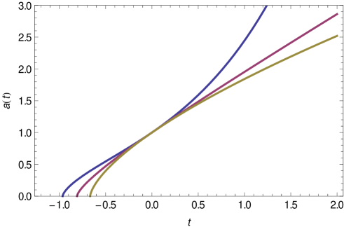
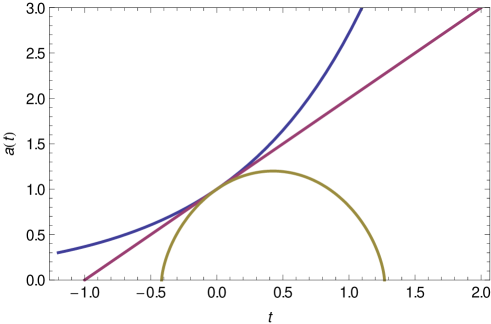
Figure 2.1: Solutions of the Friedmann equation demonstrating the evolution of the Universe. We have set the Hubble constant $H_{0}$ to unity for convenience, which implies that $t=-1$ corresponds to the Hubble time $-13.9\,\mathrm{Gyr}$. All curves pass $t=0$ (today) with $a(0)=\dot{a}(0)=1$. Top panel: From the top: The expansion history and future for our Universe with $(\Omega_{m}=0.3,\Omega_{\Lambda}=0.7)$, an open matter-only Universe $(0.3,0)$ and the Einstein–de Sitter model $(1,0)$. Bottom panel: Some more exotic solutions: A pure cosmological constant $(0,1)$, the Milne model $(0,0)$ and a closed Universe $(6,0)$.

Several decades later, the highest authority in physics—the experiment—put an end to all speculations. In the late 1990s Riess et al. (1998) observed ten supernovae of type Ia that they used as standard candles to infer their luminosity distance as a function of redshift and found that they were on average 10%–15% farther away than one would expected in an open, mass dominated Universe. They were able to rule out the $\Omega_{\Lambda}=0$ case at the $9\sigma$ confidence level, leading the way for precision cosmology. Almost simultaneously, an independent measurement by Perlmutter et al. (1998) confirmed their findings by analyzing 42 high–redshift supernovae of type Ia. Thus, the notion that the expansion of the Universe was accelerating was confirmed. Our failure to understand the nature of this accelerated expansion is reflected in the name for this phenomenon: dark energy. It is important to stress that the underlying physical cause of the acceleration does not have to be a new form of energy, it might as well be a new form of physics that mimics the effects of a cosmological constant, which is often misunderstood even by physicists unfamiliar with cosmology. Whether we are faced with a “physical darkness or dark physics”, to say it with the words of Huterer and Linder (2007), is the whole crux of the matter. Evidence independent of the distance-luminosity relation for type 1a supernovae which supports the idea of acceleration has steadily increased since the findings of Riess and Perlmutter. For instance, the late integrated Sachs-Wolfe effect (Scranton et al., 2003), or the cosmic microwave background radiation (Komatsu et al., 2010) and a dark energy component is part of today’s standard model of the Universe. But does this mean that cosmology as a science is done?

On the contrary. Even though the so called flat $\Lambda$CDM model (cold dark matter with a cosmological constant) with only six free parameters ($\omega_{m}$,$\omega_{b}$,$\Omega_{\Lambda}$,$n_{s}$,$\sigma_{8}$,$\tau$) agrees remarkably well with all observations, most physicists are still not satisfied with it for a number of reasons. First of all, the value of the cosmological constant is incredibly small. When we express $\Lambda$ in natural units, i.e. where the Planck length $l_{P}=\sqrt{\hbar G}=1$, we get $\Lambda=3.5\times 10^{-122}$. Even worse, when we interpret the cosmological constant simply as the vacuum energy predicted from quantum field theory, the value diverges. Because it is widely believed that new physics are needed at the Planck scale where neither quantum effects nor gravity are negligible, namely a theory of quantum gravity (Carroll et al., 1992), one can renormalize the integral over all modes of a scalar, massive field (e.g. a spinless boson) with zero point energy $\hbar\omega/2$ by introducing a cutoff at Planck length. This generates a finite value, but one that is still 120 orders of magnitude too large, making it arguably the worst prediction in the history of physics. Finding a mechanism that would cause fields to cancel out each other’s contributions to the vacuum energy density would be a challenge, but a mechanism that leaves a tiny, positive value seems completely out of reach for now. The most promising resolution might lie in super symmetry, super gravity or super string theory. This is commonly referred to as the cosmological constant problem (Weinberg, 1989).

The second problem is the coincidence problem, which describes the curious fact that we live exactly in a comparably short era in which matter surrenders its dominance to dark energy. This can be visualized if we consider the time dependence of the dimensionless dark energy density:

$$\Omega_{\Lambda}(a)=\frac{\rho_{\Lambda}}{\rho_{\mathrm{crit}}(a)}=\frac{\rho_{\Lambda}}{\rho_{m}(a)+\rho_{\Lambda}}=\frac{1}{\frac{\rho_{m}(a_{0})}{\rho_{\Lambda}}a^{-3}+1}\approx\frac{1}{\frac{3}{7}a^{-3}+1},$$ (2.7)

because $\rho_{m}$ scales as $a^{-3}$ while $\rho_{\Lambda}$ stays constant, when $a_{0}$ is the scale factor today, usually normalized to unity. Plotting this with its derivative on a logarithmic scale (see fig. 2.2) shows the coincidence.

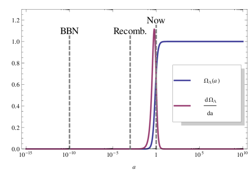
Figure 2.2: Visualization of the coincidence problem. Shown here is the dimensionless dark energy density $\Omega_{\Lambda}(a)$ in dependence of the scale factor $a$ and its derivative on a logarithmic scale. Highlighted with dashed lines are the times of big bang nucleosynthesis (BBN) at $a\approx 10^{-10}$, recombination at $a\approx 1/1000$ and today at $a=1$. Dark energy started to dominate right when structures emerged in the Universe.

Until now, there is no satisfactory solution to these problems. String theorists argue that we might live in one of $10^{500}$ realizations of the Universe, corresponding to the number of false vacua that are allowed by string theory (Douglas, 2003). This approach comes down to an anthropic argument, stating that it is no surprise that the cosmological constant has the value that it has, since any other value might be realized in a different Universe, but would not lead to the growth of structure required for sentient life that can ponder the value of natural constants (Susskind, 2005). This argument is controversial amongst physicists. As one of the leading cosmologists Paul Steinhard puts it in a Nature article (Brumfiel, 2007): “Anthropics and randomness don’t explain anything.”

Alternative theories include the postulation of Quintessence, a new kind of energy in the form of a scalar field with tracker solutions mimicking a cosmological constant (Zlatev et al., 1999), or a modification of Einstein’s theory of general relativity, where, in the most popular case, the Ricci scalar in general relativity is replaced as the Lagrangian by some function $f(R)$ (De Felice and Tsujikawa, 2010). Unfortunately, current observational constraints are insufficient when it comes to discriminating between competing theories.

2.2 Weak lensing

When light passes through a gravitational potential, its trajectory is bent in a way described by general relativity. This process, dubbed “lensing”, can alter the shape, size and brightness of the original image. We usually distinguish between strong, weak and micro lensing. The mechanism of micro lensing relies on small objects of low magnitude being the lens, such as brown or white dwarfs, neutron stars, planets and so on, that transit a bright source and temporarily increase the source’s brightness on time scales of several seconds to several years (Paczynski, 1996). The other two cases are static on those time scales, since more massive lenses like galaxies or clusters are involved, which means that the distances involved are several orders of magnitude larger. Strong lensing occurs when multiple images of the same galaxy from behind a super massive object can be observed, as seen in the bottom left corner of the left panel in fig. 2.3.

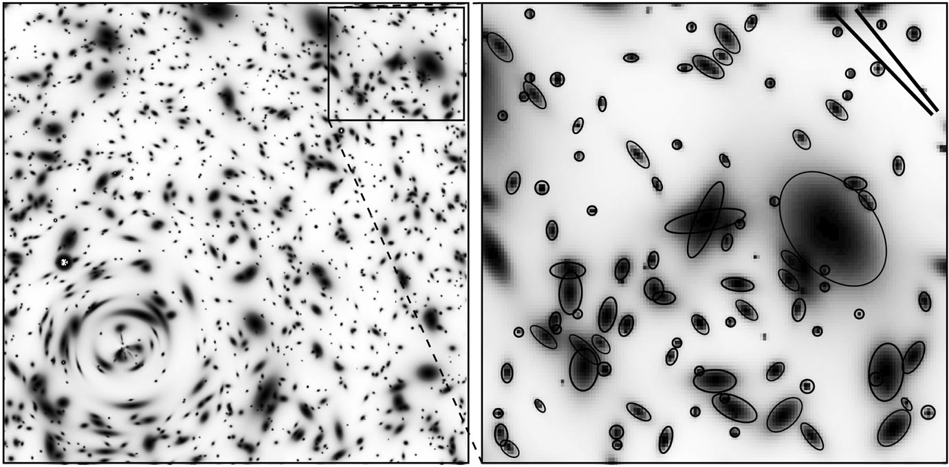
Figure 2.3: Left panel: Simulation of a gravitational lens with a case of strong lensing in the lower left corner at an average redshift of one. Right panel: Enhancement of the upper right section of the left panel, depicting lensing in the weak regime. The contours are ellipses derived from the quadrupole moment of each galaxy image. The two bars in the upper right corner show the average shear, where the lower one represents the expected shear and the upper one the actual shear. The deviation stems from shot noise due to the intrinsic ellipticity and random orientation of the galaxies. Taken from Mellier (1998).

While strong and micro lensing are relatively rare, weak lensing is an effect that can be observed over large areas of the sky (see upper right corner of the right panel in fig. 2.3). Its power lies in statistical analysis, since weakly lensed objects are only slightly distorted and impossible to detect individually. Only the average distortion field reveals the cosmological information that we are looking for. As it turns out, weak lensing changes the ellipticity of galaxies (in a first order approximation), but the intrinsic ellipticity always dominates the shape. We need to gather large enough samples and then subtract the noise, which is relatively simple if the magnitude and direction of the intrinsic ellipticity is uncorrelated to the signal. This is unfortunately not entirely the case due to tidal effects (intrinsic alignment), and this is only one of the many challenges that weak lensing harbors. The most obvious one is illustrated in fig. 2.4. Others include photometric redshift errors, calibration errors and uncertainties in power spectrum theory. A lot of these systematic errors can be accounted for by introducing several nuisance parameters (Bernstein, 2009). The trade-off is that a high number of nuisance parameters diminish the merit of the Fisher matrix formalism, as there are degeneracies to be expected, so we will only account for photometric redshift error and the intrinsic ellipticity in this thesis.

a) b) c) d) e)

Figure 2.4: A schematic illustration of the process of weak lensing detection, demonstrating its difficulty. a) The original source galaxy. b) Weak lensing distorts the shape and adds a shear to the image. c) The image is convolved by the telescopes point spread function and, in case of ground based surveys, the atmosphere. d) The effect of the finite resolution of the detector. e) Additional noise is applied to the image. The challenge now is to infer b) from e). (Image of M31 by courtesy of Robert Gendler.)

An expression describing the shear can be obtained by perturbing the Friedmann-Lemaître-Robertson-Walker metric in the Newtonian gauge

$$\,\mathrm{d}s^{2}=-(1+2\Psi)\,\mathrm{d}t^{2}+a^{2}(t)(1+2\Phi)(\,\mathrm{d}x_{1}^{2}+\,\mathrm{d}x_{2}^{2}+\,\mathrm{d}x_{3}^{2})\,,$$ (2.8)

where $\Psi$ and $\Phi$ are scalar gravitational potentials. We can then solve the geodesic equation for a light ray

$$\frac{\,\mathrm{d}k^{\mu}}{\,\mathrm{d}\lambda}+\Gamma_{\alpha\beta}^{\mu}k^{\alpha}k^{\beta}=0\,,$$ (2.9)

which can be rewritten in our case as

$$\frac{\,\mathrm{d}^{2}}{\,\mathrm{d}r^{2}}(r\theta_{i})=\Phi_{,i}-\Psi_{,i}\,.$$ (2.10)

Thus, we obtain the lensing equation

$$\theta_{i}=\theta_{0i}+\int_{0}^{r}\,\mathrm{d}r^{\prime}\left(1-\frac{r^{\prime}}{r}\right)\phi_{,i}(r^{\prime}\theta_{01},r^{\prime}\theta_{02},r^{\prime})$$ (2.11)

with the lensing potential $\psi=\Phi-\Psi$. Here $r$ is the radial comoving coordinate, $\theta_{i}=x_{i}/r$ is the angle of the light ray with respect to the $r$-axis, and $(x_{1},x_{2})$ are displacement coordinates perpendicular to the $r$-axis.

Figure 2.5: Description of the lensing configuration. Note that comoving distances cannot be added trivially, i.e. $r_{s}\neq r_{l}+r_{ls}$.

The distortion of a source image at distance $r_{s}$ to first order is a linear transformation described by the symmetric matrix

$$A_{ij}\equiv\frac{\partial\theta_{si}}{\partial\theta_{0j}}=\delta_{ij}+D_{ij}$$ (2.12)

with

$$D_{ij}(r_{s})=\int_{0}^{r_{s}}\,\mathrm{d}r^{\prime}\left(1-\frac{r^{\prime}}{r_{s}}\right)r^{\prime}\psi_{,ij}=\left(\begin{array}[]{cc}-\kappa_{\mathrm{wl}}-\gamma_{1}&-\gamma_{2}\\ -\gamma_{2}&-\kappa_{\mathrm{wl}}+\gamma_{1}\end{array}\right)\,.$$ (2.13)

Here we introduced the convergence

$$\kappa_{\mathrm{wl}}=-\frac{1}{2}\int_{0}^{r_{s}}\,\mathrm{d}r^{\prime}\left(1-\frac{r^{\prime}}{r_{s}}\right)r^{\prime}(\psi_{,11}+\psi_{,22})\,,$$ (2.14)

which is a measure for the magnification of the image, and the shear

$$\gamma_{1} =-\frac{1}{2}\int_{0}^{r_{s}}\,\mathrm{d}r^{\prime}\left(1-\frac{r^{\prime}}{r_{s}}\right)r^{\prime}(\psi_{,11}-\psi_{,22})\,,$$ (2.15)

$$\gamma_{2} =-\int_{0}^{r_{s}}\,\mathrm{d}r^{\prime}\left(1-\frac{r^{\prime}}{r_{s}}\right)r^{\prime}\psi_{,12}\,,$$ (2.16)

which describes the distortion. These quantities will become important when we want to describe the cosmic shear by statistical means, in particular its power spectrum.

We can measure the ellipticity of real astronomical images by computing their quadrupole moment, which is defined as

$$q_{ij}=\int I(\bm{\theta})\theta_{i}\theta_{j}\,\mathrm{d}^{2}\theta\,,$$ (2.17)

where $I(\bm{\theta})$ is the luminous intensity of the galaxy image with its center at $\bm{\theta}=0$. The complex ellipticity is then given by

$$\chi\equiv\frac{q_{11}-q_{22}+2iq_{12}}{q_{11}+q_{22}}\,.$$ (2.18)

It is straight forward to show that according to this definition the complex ellipticity for an ellipse with semiaxes $a$ and $b$, rotated by an angle $\phi$, is

$$\chi=\frac{a^{2}-b^{2}}{a^{2}+b^{2}}e^{2i\phi}\,.$$ (2.19)

To first order, a weak lens distorts a spherical object into an ellipse with a simple relation between the shear and the complex ellipticity, namely

$$\chi=2(\gamma_{1}+i\gamma_{2})\,.$$ (2.20)

We can use this to compute the power spectra $P_{\gamma_{i}}(\ell)$, which describe the auto-correlation of the shear field at the multipole $\ell$, the adjoint variable to $\theta$. It can be shown that the convergence power spectrum $P$ is related to the matter power spectrum and can be written to first order as a linear combination $P=P_{E}=c_{1}P_{\gamma_{1}}+c_{2}P_{\gamma_{2}}$. Another linear combination, $P_{B}=c_{1}P_{\gamma_{1}}-c_{2}P_{\gamma_{2}}$, must vanish. These are usually referred to as the electric and magnetic part of the shear field. Thus, the convergence power spectrum contains all the information while the magnetic part provides a good check for systematics.

But, as mentioned before, not all galaxies appear circular even if their intrinsic shape was a perfectly circular disc and there was no gravitational lensing distorting our view of the sky, as they are randomly oriented and thus, viewed from the side, look like ellipses. This intrinsic ellipticity, denoted by $\gamma_{\mathrm{int}}$, can be reflected in a noise term that is added to the power spectrum, if we assume that the noise is uncorrelated to the weak lensing signal:

$$P=P_{\mathrm{signal}}+\gamma_{\mathrm{int}}^{2}n^{-1}\,,$$ (2.21)

where $n$ is the average galaxy density (A&T, ch. 14.4).

The shear field is a vector field of dimension two. To access the full power of weak lensing, we must also include the third dimension, which can be done by considering the redshift of each source galaxy. Weak lensing works linearly, so we can add up the transformation matrices of all galaxies and find for the full transformation matrix

$$\mathcal{D}_{ij}=\int_{0}^{\infty}\,\mathrm{d}r^{\prime}n(r^{\prime})D_{ij}(r^{\prime})\,,$$ (2.22)

where $n(r)\,\mathrm{d}r$ is the number of galaxies in a shell with width $\,\mathrm{d}r$ and the galaxy distribution function $n(r)$ is normalized to unity. Making use of the fact that for any real, integrable functions $f(x)$ and $g(x,y)$ the identity

$$\int_{0}^{\infty}\,\mathrm{d}xf(x)\int_{0}^{x}\,\mathrm{d}yg(x,y)=\int_{0}^{\infty}\,\mathrm{d}y\int_{y}^{\infty}\,\mathrm{d}xf(x)g(x,y)$$ (2.23)

holds, we can rewrite eq. (2.22) to get

$$\mathcal{D}_{ij}=\int_{0}^{\infty}\,\mathrm{d}rw(r)\psi_{,ij}\,.$$ (2.24)

Here we abbreviated the weight function as

$$w(r)\equiv\int_{r}^{\infty}\,\mathrm{d}r^{\prime}\left(1-\frac{r}{r^{\prime}}\right)rn(r^{\prime})\,.$$ (2.25)

Thus, the total convergence field from eq. (2.14) now reads

$$\kappa_{\mathrm{wl}}=-\frac{1}{2}\int_{0}^{\infty}\,\mathrm{d}rw(r)\left(\psi_{,11}+\psi_{,22}\right)\,.$$ (2.26)

By grouping all observed galaxies into redshift bins, we are able to extract more information out of the given data by calculating the power spectrum in each each redshift bin as well as their cross correlation. This is called power spectrum tomography (Hu, 1999). We shall cover this in more detail in section 3.1.

2.3 Power spectra

Almost every book and every lecture on modern cosmology begins with the cosmological principle: the assumption that the Universe is, simply put, homogeneous and isotropic. Now obviously the average density, say, $100\,\mathrm{m}$ below the University Square in Heidelberg is quite different than the average density $100\,\mathrm{m}$ above, and it is still quite different at the midpoint between the Sun and Alpha Centauri – we say that the Universe has structure. But if we look at the Universe at sufficiently large scales of $\gtrsim 1\,\mathrm{Gpc}$, the overall success of the standard model confirms our initial assumption (Komatsu et al., 2010). While there are research groups who investigate the possibility of genuine large scale inhomogeneities (Barausse et al., 2005; Kolb et al., 2005), we remain confident that there is good reason to believe that the cosmological principle applies to the Universe as a whole.

The matter distribution in tour Universe consists mostly of structures at different scales, which can be roughly classified as voids, super clusters, clusters, groups, galaxies, solar systems, stars, planets, moons, asteroids and so on. This “lumpiness” is inherently random, but like all randomness it can be characterized by an underlying set of well defined rules by using statistics. The matter distribution in our Universe is one sample drawn from an imaginary ensemble of Universes with an according probability distribution function (PDF), and we are now facing the challenge of determining that PDF.

We require our models to make precise predictions regarding the structure of matter. Naturally, no model will be able to predict the distance between the Milky Way and Andromeda for instance, but it should be able to predict how likely it is for two objects of that size to have the separation that they have. To quantify and measure the statistics of the irregularities in the matter distribution in the cosmos, we define the two-point correlation function $\xi$ as the average of the relative excess number of pairs found at a given distance. That is, if $n_{i},\,i\in\{1,2\},$ denotes the number of point-like objects (nucleons, or galaxies, or galaxy clusters) found in some volume element $\,\mathrm{d}V_{i}$ at position $\bm{r}_{i}$ with a sample average $\langle n_{i}\rangle=n_{0}\,\mathrm{d}V_{i}$, we can write the average number of pairs found in $\,\mathrm{d}V_{1}$ and $\,\mathrm{d}V_{2}$ as

$$\langle n_{1}n_{2}\rangle=n_{0}^{2}\,\mathrm{d}V_{1}\,\mathrm{d}V_{2}[1+\xi(\bm{r}_{1},\bm{r}_{2})],$$ (2.27)

where $n_{0}=N/V$ is the mean number density. If the matter distribution was truly random, then any two volume elements would be uncorrelated, which means that $\xi$ would vanish and the average number of pairs would simply be the product of the average amount of objects in each volume element. If $\xi$ is positive (negative), then we say those two volume elements are correlated (anti-correlated).

Assuming a statistically homogeneous Universe, $\xi$ can only depend on the difference vector $\bm{r}_{12}=\bm{r}_{2}-\bm{r}_{1}$. Further assuming statistical isotropy allows $\xi$ to only depend on the distance $r$ between $\bm{r}_{1}$ and $\bm{r}_{2}$. Hence, we denote the two-point correlation function as $\xi(r)$. Solving eq. (2.27) leads to

$$\xi(|\bm{r}_{2}-\bm{r}_{1}|)=\frac{\langle n_{1}n_{2}\rangle}{n_{0}^{2}\,\mathrm{d}V_{1}\,\mathrm{d}V_{2}}-1=\langle\delta_{m}(\bm{r}_{1})\delta_{m}(\bm{r}_{2})\rangle,$$ (2.28)

which can be easily checked by plugging in the definition of the density contrast

$$\delta_{m}\left(\bm{r}_{i}\right)=\frac{n_{i}-\langle n_{i}\rangle}{\langle n_{i}\rangle}.$$ (2.29)

Thus, the correlation function is often written as the average over all possible positions

$$\xi(|\bm{r}|)=\frac{1}{V}\int_{V}\delta_{m}(\bm{x})\delta_{m}(\bm{x}+\bm{r})\,\mathrm{d}^{3}x.$$ (2.30)

Another important tool that will later prove to be invaluable is the power spectrum, which is in a cosmological context the square of the Fourier transform of a perturbation variable (up to some normalization constant). For instance, the matter power spectrum is defined as

$$P_{m}(\bm{k})\equiv V\tilde{\delta}_{m}(\bm{k})\tilde{\delta}_{m}^{*}(\bm{k})=\frac{1}{V}\left|\int\delta_{m}(\bm{x})e^{-i\bm{k}\cdot\bm{x}}\,\mathrm{d}^{3}x\right|^{2}.$$ (2.31)

Rewriting the norm yields

$$P_{m}(\bm{k})=\frac{1}{V}\int\delta_{m}(\bm{x})\delta_{m}(\bm{y})e^{-i\bm{k}\cdot(\bm{x}-\bm{y})}\,\mathrm{d}^{3}x\,\mathrm{d}^{3}y$$ (2.32)

or, if we substitute $\bm{r}=\bm{x}-\bm{y}$

$$P_{m}(\bm{k})=\frac{1}{V}\int\delta_{m}(\bm{x})\delta_{m}(\bm{x}-\bm{r})e^{-i\bm{k}\bm{r}}\,\mathrm{d}^{3}x\,\mathrm{d}^{3}r=\int\xi(r)e^{-i\bm{k}\bm{r}}\,\mathrm{d}^{3}r\,,$$ (2.33)

where we used eq. (2.30) in the last step. Hence the power spectrum is the Fourier transform of the two-point correlation function.

The power spectrum is amongst the cosmologist’s favorite tool to describe our Universe in a meaningful way. It is often applied for instance to the matter distribution, the anisotropies of the cosmic microwave background radiation or the shear field of weak lensing.

The convergence power spectrum describing the cosmic shear of galaxy images can be expressed in terms of the matter power spectrum. Since the matter distribution is 3-dimensional, but the convergence is a function of the 2-dimensional sky, we need Limber’s theorem to relate those two. It states that the power spectrum for a projection

$$F(\theta_{x},\theta_{y})=\int_{0}^{\infty}w(r)f(\theta_{x}r,\theta_{y}r,r)\,\mathrm{d}r\,,$$ (2.34)

where $w(r)$ is a weight function (normalized to unity), turns out to be

$$P(q)=\int_{0}^{\infty}\,\mathrm{d}r\frac{w(r)^{2}}{r^{2}}p\left(\frac{q}{r}\right)\,,$$ (2.35)

where $p(k)$ is the power spectrum of $f$. This theorem is directly applicable to the total convergence field in eq. (2.26), so that its power spectrum becomes

$$P_{\kappa_{\mathrm{wl}}}(q) =\frac{1}{4}\int_{0}^{\infty}\,\mathrm{d}r\frac{w(r)^{2}}{r^{2}}P_{\Sigma_{i}\psi_{,ii}}\left(\frac{q}{r}\right)$$ (2.36)

$$=\frac{1}{4}\int_{0}^{\infty}\,\mathrm{d}z\frac{W(z)^{2}}{H(z)}P_{\Sigma_{i}\psi_{,ii}}\left(\frac{q}{r}\right)$$ (2.37)

with

$$W(z)\equiv\frac{w(r(z))}{r(z)}$$ (2.38)

being the window function. All we need to know now is the power spectrum of $\psi_{,ij}$, which is simply

$$P_{\psi_{,ij}}=k_{i}^{2}k_{j}^{2}|\tilde{\psi}|^{2}$$ (2.39)

because the Fourier transform of $\psi_{,ij}$ is $-k_{i}k_{j}\tilde{\psi}$. Then we can plug in the Poisson equation in Fourier space, which is

$$k^{2}\tilde{\psi}=3a^{2}H(a)^{2}\Omega(a)\delta_{m}(a)$$ (2.40)

(in the absence of anisotropic stress, i.e. $\psi=2\Phi$) to obtain

$$P_{\Sigma_{i}\psi_{,ii}}(k)=k^{4}\tilde{\psi}=9H(a)^{4}\Omega_{m}^{2}/(1+z)^{4}P_{m}(k)\,.$$ (2.41)

Putting it all together, and replacing $q$ with the multipole $\ell/\pi$, finally yields the power spectrum for the convergence,

$$P(\ell)=\frac{9H_{0}^{3}}{4}\int_{0}^{\infty}\frac{W(z)^{2}E(z)^{3}\Omega_{m}(z)^{2}}{(1+z)^{4}}P_{m}\left(\frac{\ell}{\pi r(z)}\right)\,\mathrm{d}z\,.$$ (2.42)

More details can be found in A&T (ch. 4.11, 14.4) or Hu and Jain (2004).

In fig. 2.6 we can see the matter power spectrum derived from linear perturbation theory as well as non-linear corrections. Fig. 2.6 shows the convergence power spectrum, derived from the linear and non-linear matter power spectrum according to eq. (2.42).

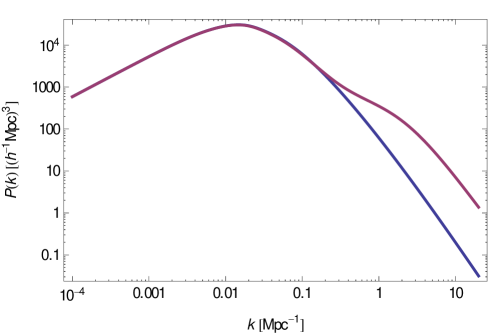
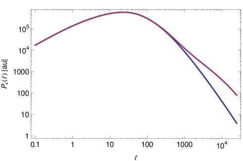
Figure 2.6: Top panel: Comparison between a matter power spectrum with (purple) and without (blue) non-linear corrections in arbitrary units. The fitting formulae were taken from Eisenstein and Hu (1999) and Smith et al. (2003). Non-linear corrections become important only at wave numbers $k>0.1\,\mathrm{Mpc}^{-1}$. Note that $k$ is not in units of $h\,\mathrm{Mpc}^{-1}$ in this case. Bottom panel: Comparison between a convergence power spectrum from eq. (2.42) based on the linear and non-linear matter power spectrum (no redshift binning).

2.4 Fisher matrix formalism

The last tool we will need is the powerful theory of Bayesian statistics. In physics we define a theory by a set of parameters encapsulated in the vector $\bm{\theta}$. The ultimate goal is to deduce the value of $\bm{\theta}$ by performing a series of experiments that yield the data $\bm{x}$. If we were given the values of $\bm{\theta}$, we could calculate the probability density function $f(\bm{x},\bm{\theta})$ and thus predict the probability $P$ of getting a realization of the data $\bm{x}$ given the theory $\bm{\theta}$, which is usually denoted by $P(\bm{x}|\bm{\theta})$. But since we rarely are given the exact theory, all we can do is draw samples $\bm{x}_{i}$ of an unknown PDF by conducting experiments in order to estimate the parameters $\bm{\theta}$. In a frequentist approach, we would take those parameters as the true ones that maximize the so-called likelihood function

$$\mathcal{L}(\bm{\theta},\bm{x}_{i})\equiv\prod\limits_{i}f(\bm{x}_{i},\bm{\theta})\,,$$ (2.43)

which is nothing but the joined PDF, with $\bm{\theta}$ now being interpreted as a variable and $\bm{x}$ as a fixed parameter. But in cosmology, we often have prior knowledge about the parameters from other observations or theories that we would like to account for. For this, we need Bayes’ theorem:

$$P(\bm{\theta}|\bm{x},I)=\frac{P(\bm{\theta}|I)P(\bm{x}|\bm{\theta},I)}{P(\bm{x}|I)}\,.$$ (2.44)

In this Bayesian approach, we turn the situation around so that we are asking the question: What is the probability of the theory, given the observed data? Note that we included the background information $I$ in every term even though it is hardly relevant to the derivation. It is to remind ourselves that we always assume some sort of prior knowledge, even when we do not realize it. For instance, we might implicitly assume that the Copernican principle holds true, or that the Universe is described by the Einstein field equations.

Here the prior knowledge (or just prior) is given by $P(\bm{\theta}|I)$, and $P(\bm{x}|I)$ is the marginal probability of the data $\bm{x}$ which acts as a normalization factor, requiring that $\int\mathcal{L}(\bm{\theta},\bm{x}_{i})\,\mathrm{d}^{n}\theta=1$. $P(\bm{x}|\bm{\theta},I)$ is identical to the likelihood, which is given by the model. This could be for instance a Gaussian PDF

$$\prod\limits_{i=1}^{n}\frac{1}{\sigma_{i}\sqrt{2\pi}}\exp\left(-\frac{(\hat{x}_{i}-x_{i}(\bm{\theta}))^{2}}{2\sigma_{i}^{2}}\right)\,.$$ (2.45)

The left hand side of eq. (2.44) is then called the posterior (Hobson et al., 2009, p. 42). We now have all the ingredients to calculate the posterior probability of the parameters given the data. This quantity is important for computing the so-called evidence, which is defined by the integral over the numerator in eq. (2.44) and needed for model selection.

Unfortunately, the likelihood is often not a simple Gaussian. Finding the values of $\bm{\theta}$ that maximize the PDF given by eq. (2.44) can be computationally demanding, since a (naïve) algorithm for finding the extremum scales exponentially with the number of dimensions of the parameter space. This will becomes a problem when considering 30 parameters as we will later in this thesis. It is not unusual for Bayesian statistics to suffer from the “curse of dimensionality”(Bellman, 2003). One way to overcome this curse is by using Markov chain Monte Carlo methods. In the case of a likelihood that is not a multivariate Gaussian, we can simply assume that it can at least be approximated by one. This is not an unreasonable assumption, since the logarithm of the likelihood can always be Taylor expanded up to the second order around its maximum, denoted by $\hat{\bm{\theta}}$:

$$\ln\mathcal{L}(\bm{\theta})\approx\ln\mathcal{L}(\hat{\bm{\theta}})+\frac{1}{2}\sum\limits_{i,j}\left.\frac{\partial^{2}\ln\mathcal{L}(\bm{\theta})}{\partial\theta_{i}\partial\theta_{j}}\right|_{\bm{\theta}=\hat{\bm{\theta}}}(\theta_{i}-\hat{\theta}_{i})(\theta_{j}-\hat{\theta}_{j})\,.$$ (2.46)

No first order terms appear since they vanish in a maximum by definition. It is now quite useful to define the Fisher matrix as the negative of the Hessian of the likelihood,

$$F_{ij}\equiv-\left.\frac{\partial^{2}\ln\mathcal{L}(\bm{\theta})}{\partial\theta_{i}\partial\theta_{j}}\right|_{\bm{\theta}=\hat{\bm{\theta}}}\,.$$ (2.47)

This definition is not very useful when we need to find the maximum of a multi-dimensional function and then compute the derivatives numerically anyway, since many expensive evaluations is what we wanted to avoid in the first place. However, since this thesis deals with constraints by future surveys, using some fiducial model which we already know the expected outcome of and thus the peaks of the likelihood. This is the reason why the Fisher matrix is a perfect tool in assessing the merit of future cosmological surveys.

Let us consider a survey in which we measure some set of observables $\bm{x}$ (along with their respective standard errors $\bm{\sigma}$) whose theoretical values $\hat{\bm{x}}(\bm{\theta})$ depend on our model. These observables could be the same quantity at different redshifts, i.e. $x_{i}=x(z_{i})$, or different quantities all together, e.g. $\bm{x}=(z_{\mathrm{CMB}},c_{s},\Omega_{k})$, or a mixture of both. Assuming a Gaussian PDF we can write down the likelihood as

$$\mathcal{L}(\bm{\theta})\propto\exp\left(-\frac{1}{2}\sum\limits_{i}\frac{(x_{i}-\hat{x_{i}}(\bm{\theta}))^{2}}{\sigma_{i}^{2}}\right)\,.$$ (2.48)

Using the definition in eq. (2.47) we get for the Fisher matrix

$$F_{ij}=-\sum\limits_{k}\left.\frac{1}{\sigma_{k}^{2}}\frac{\partial^{2}\hat{x}_{k}(\bm{\theta})}{\partial\theta_{i}\partial\theta_{j}}\right|_{\bm{\theta}=\hat{\bm{\theta}}}\,.$$ (2.49)

2.4.1 Calculation rules

We will not go into a full derivation of the rules, as they can be found in A&T (ch. 13.3) and are quite straight forward, but rather simply state them here.

Fixing a parameter.

If we want to know what the Fisher matrix would be given that we knew one particular parameter $\theta_{i}$ precisely, we simply remove the $i$-th row and column of the Fisher matrix.

Marginalizing over a parameter.

If, on the other hand, we want to disregard a particular parameter $\theta_{i}$, we remove $i$-th row and column from the inverse of the Fisher matrix (the so-called correlation matrix) and invert again afterwards. If we are only interested in exactly one parameter $\theta_{i}$, then we cross out all other rows and columns until the correlation matrix only has one entry left. Thus, we arrive at the important result

$$\sigma(\theta_{i})^{2}=(\mathbf{\mathsf{F}}^{-1})_{ii}\,.$$ (2.50)

This implies that the Fisher matrix must be positive definite, as it must be as the Hessian in a maximum.

Combination of Fisher matrices.

Including priors in our analysis is extremely simple in the Fisher matrix formalism, since all we need to do is add the Fisher matrix:

$$\mathbf{\mathsf{F}}^{\prime}=\mathbf{\mathsf{F}}+\mathbf{\mathsf{F}}^{\mathrm{prior}}\,.$$ (2.51)

This only holds if both matrices have been calculated with the same underlying fiducial model, i.e. the maximum likelihood is the same. The only difficulty lies in ensuring that the parameters of the model belonging to each matrix are identical and line up properly. If one matrix covers additional parameters, then the other matrix must be extended with rows and columns of zeros accordingly.

Parameter transformation.

Often a particular parameterization of a model is not unique and there exists a transformation of parameters

$$\bm{\theta}^{\prime}=\bm{\theta}^{\prime}(\bm{\theta})\,,$$ (2.52)

which might happen when combining Fisher matrices from different sources. Then the Fisher matrix transforms like a tensor, i.e.

$$\mathbf{\mathsf{F}}^{\prime}=\mathbf{\mathsf{J}}^{T}\mathbf{\mathsf{F}}\mathbf{\mathsf{J}}\,,$$ (2.53)

where $\mathbf{\mathsf{J}}$ is the Jacobian matrix

$$J_{ij}=\frac{\partial\theta_{i}}{\partial\theta_{j}^{\prime}}\,,$$ (2.54)

which does not necessarily need to be a square matrix. If it is not, however, note that the new Fisher matrix will be degenerate and using it only makes sense when combining it with at least one matrix from a different source.

Chapter 3 Constraints on cosmological parameters by future dark energy surveys

With the knowledge of the observational specifications of future weak lensing surveys, we can use the Fisher matrix formalism to forecast the errors that said surveys will place on cosmological parameters. In particular, we want to expand the list of those parameters with values of the Hubble parameter and growth function at certain redshifts. An invaluable resource for this chapter is the book by A&T (ch. 14)

3.1 Power spectrum tomography

It has been shown that dividing up the distribution of lensed galaxies into redshift bins and measuring the convergence power spectrum in each of these bins as well as their cross-correlation can increase the amount of information extracted from weak lensing surveys (Hu, 1999; Huterer, 2002). This means on one hand that we need to have additional redshift information on the lensed galaxies, but on the other that we are possibly rewarded with gaining knowledge about the evolution of dark energy parameters. Note that the purpose of the redshift bins in this thesis is two-fold, and power spectrum tomography is only one of them. The other is the linear interpolation of $H(z)$ and $G(z)$, where the centers of the redshift bins act as supporting points, making our analysis independent of assumptions about the growth function by any particular model. We choose to divide the redshift space into $\mathcal{N}$ bins such that each redshift bin contains roughly the same amount of galaxies according to the galaxy density function $n(z)$, i.e.

$$\int_{z_{i-1}}^{z_{i}}n(z)\,\mathrm{d}z=\frac{1}{\mathcal{N}}\int_{0}^{\infty}n(z)\,\mathrm{d}z$$ (3.1)

for each $i$. We infer the values of the $z_{i}$ via a series of successive numerical integrations with $z_{0}=0$ and $z_{\mathcal{N}}=3$ (see fig. reffig:2-zbins). A common parametrization of $n(z)$ is

$$n(z)\propto z^{\alpha}e^{-\left({z}/{z_{p}}\right)^{\beta}},$$ (3.2)

with $\alpha=2$ and $\beta=\frac{3}{2}$. Here $z_{p}$ is related to the median redshift $z_{m}=1.412z_{p}$ (Amara and Refregier, 2007).

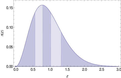
Figure 3.1: The area under the curve of the galaxy density function is the same in each redshift bin for $\mathcal{N}=5$.

We need a galaxy density function for each bin, and the naïve choice would be

$$\hat{n}_{i}(z)=\left\{\begin{array}[]{ll}n(z)&z_{i-1}<z\leq z_{i}\,,\\ 0&\mathrm{else.}\end{array}\right.$$ (3.3)

But to account for redshift measurement uncertainties, we will convolve $\hat{n}(z)$ with the probability distribution of the measured redshift $z_{\mathrm{ph}}$ given the real value $z$:

$$n_{i}(z)=\int_{0}^{\infty}\,\mathrm{d}z^{\prime}\hat{n}_{i}(z^{\prime})P_{i}(z_{\mathrm{ph}}=z^{\prime}|z)\,.$$ (3.4)

Note that the integral vanishes if $z^{\prime}$ lies outside the $i$th bin, so the limits can be adjusted to the according finite values. This convolution reflects the fact that we cannot assign a galaxy to a particular bin by measuring the photometric redshift with finite precision. The probability distribution is here modeled by Gaussian, i.e.

$$P_{i}(z_{\mathrm{ph}}|z)=\frac{1}{\sqrt{2\pi}\sigma_{i}}\exp\left(-\frac{\left(z_{\mathrm{ph}}-z\right)^{2}}{2\sigma_{i}^{2}}\right)$$ (3.5)

with $\sigma_{i}=\Delta_{z}(1+(z_{i-1}+z_{i})/2)$ (see Ma et al. (2006) for details). Finally, we normalize each function to unity, such that

$$\int_{0}^{\infty}n_{i}(z)\,\mathrm{d}z=1\,.$$ (3.6)

The resulting functions can be visualized as in fig. 3.2.

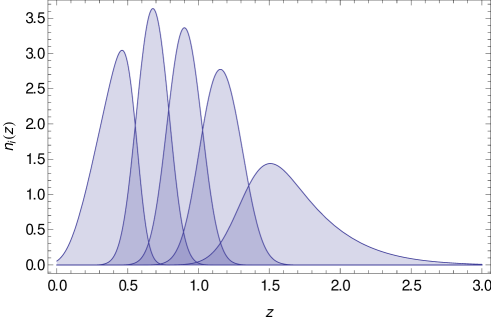
Figure 3.2: Normalized galaxy density functions for each bin with $\mathcal{N}=5$, convolved with a Gaussian to account for photometric redshift measurement errors.

3.2 The matter power spectrum

Future weak lensing surveys will supply us with the convergence power spectrum in which the cosmological information we are seeking is imprinted. However, for now we will have to rely on simulated data. As we will see in section 3.3, the convergence power spectrum depends on the matter power spectrum which can be simulated by a fitting formula derived by Eisenstein and Hu (1999). Non-linear corrections need to be accounted for, since we are assuming an angular galaxy density of $35\,\mathrm{arcmin}^{-2}$, which corresponds to a multipole up to a order of magnitude of

$$\lg\left(\sqrt{35\,\mathrm{arcmin}^{-2}}\right)\approx 4\,.$$ (3.7)

As we saw in fig. 2.6, non-linear corrections are required for $\ell\gtrsim 10^{3}$, and for this we need to use the results by Smith et al. (2003). Here we will give a brief overview of the essential results found in the two papers cited above, using our notation and some simplifications (no massive neutrinos, flat cosmology).

3.2.1 Fitting formulas

It should be stressed that the growth function $D(z)$ in Eisenstein’s paper differs from ours by a factor of $a=1/(1+z)$, so $D(z)=aG(z)$. A precise definition of the growth function will be given in section. 3.6.2. They also define $\Theta_{2.7}\equiv T_{\mathrm{CMB}}/2.7\,\mathrm{K}$. Only in this section will we differentiate between the linear and the non-linear power spectrum. Later on, the expression “power spectrum” or $P_{m}(k)$ will always imply that non-linear corrections have been applied.

Using the definition of the growth function, the matter power spectrum in the linear regime can be written as (cf. eq. (3.72))

$$P_{\mathrm{L}}(k)\propto k^{n_{s}}\frac{G(z)^{2}}{(1+z)^{2}}T(z,k)^{2}\,,$$ (3.8)

where $n_{s}$ is called the scalar spectral index. The transfer function $T(k)$ can now be fitted by a series of functions as follows.

$$T(k)=\frac{LB(k)}{L+Cq_{\mathrm{eff}}^{2}}\,,$$ (3.9)

with (we assume that there are no massive neutrinos, in which case $B(k)$ equals unity)

$$L =\ln(e+1.84\beta_{c}\sqrt{\alpha_{\nu}}q_{\mathrm{eff}})$$ (3.10)

$$C =1.44+\frac{325}{1+60.5q_{\mathrm{eff}}^{1.11}}$$ (3.11)

where

$$q_{\mathrm{eff}} =\frac{k\Theta^{2}_{2.7}}{\Gamma_{\mathrm{eff}}\,\mathrm{Mpc}^{-1}}$$ (3.12)

$$\Gamma_{\mathrm{eff}} =\omega_{m}\left(\sqrt{\alpha_{\nu}}+\frac{1-\sqrt{\alpha_{\nu}}}{1+(0.34ks)^{4}}\right)$$ (3.13)

and

$$\alpha_{\nu}=\frac{\omega_{c}}{\omega_{m}}\frac{5-2(p_{c}+p_{m})}{5-4p_{m}}\left(1-0.553\omega_{b}+0.126\omega_{b}^{3}\right)(1+y_{d})^{p_{m}-p_{c}}\\ \times\left\{1+\frac{p_{c}-p_{cb}}{2}\left[1+\frac{1}{(3-4p_{c})(7-4p_{m})}\right](1-y_{d})^{-1}\right\}\,.$$ (3.15)

Here, we used the abbreviations

$$p_{x} =\frac{1}{4}(5-\sqrt{1+24\omega_{x}})$$ (3.16)

$$y_{d} =\frac{1+z_{\mathrm{eq}}}{1+z_{d}}$$ (3.17)

with

$$z_{\mathrm{eq}} =2.50\times 10^{4}\omega_{m}\Theta_{2.7}^{-4}$$ (3.18)

$$z_{d} =1291\frac{\omega_{m}^{0.251}}{1+0.659\omega_{m}^{0.828}}(1+b_{1}\omega_{m}^{b_{2}})$$ (3.19)

$$b_{1} =0.313\omega_{m}^{-0.419}(1+0.607\omega_{m}^{0.674})$$ (3.20)

$$b_{2} =0.238\omega_{m}^{0.223}\,.$$ (3.21)

By definition, the power spectrum needs to be normalized such that

$$\sigma_{8}^{2}=\int_{0}^{\infty}\frac{\,\mathrm{d}k}{k}\frac{k^{3}}{2\pi^{2}}P_{\mathrm{L}}(k)|\tilde{W}_{8}(k)|^{2}\,,$$ (3.22)

where $\tilde{W}_{R}(k)$ is the Fourier transform of the real-space window function, in this case a spherical top hat of radius $R$ (in Mpc), i.e.

$$W_{R}(r) \propto\left\{\begin{array}[]{ll}1&\mathrm{if}\>\>r\leq R\\ 0&\mathrm{otherwise}\end{array}\right.$$ (3.25)

$$\tilde{W}_{R}(k) =\frac{3}{(kR)^{3}}(\sin kR-kR\cos kR)\,.$$ (3.26)

3.2.2 Non-linear corrections

When applying non-linear corrections, we use the dimensionless power spectrum, which is defined by

$$\Delta_{\mathrm{L}}^{2}(k)=\frac{4\pi k^{3}}{(2\pi)^{3}}P_{\mathrm{L}}(k)\,,$$ (3.27)

and similarly for other indices. It turns out that the non-linear power spectrum can be decomposed into a quasi-linear term and contributions from self-correlations

$$\Delta_{\mathrm{NL}}^{2}=\Delta^{2}_{\mathrm{Q}}(k)+\Delta^{2}_{\mathrm{H}}(k)\,,$$ (3.28)

which are given by

$$\Delta_{\mathrm{Q}}^{2}(k) =\Delta_{\mathrm{L}}^{2}(k)\left(\frac{(1+\Delta_{\mathrm{L}}^{2}(k))^{\beta_{n}}}{1+\alpha_{n}\Delta_{\mathrm{L}}^{2}(k)}\right)\exp(-y/4-y^{2}/8)$$ (3.29)

$$\Delta_{\mathrm{H}}^{2}(k) =\frac{{\Delta_{\mathrm{H}}^{2}}^{\prime}(k)}{1+\mu_{n}y^{-1}+\nu y^{-2}}\,,$$ (3.30)

with $y\equiv k/k_{\sigma}$ and

$${\Delta^{2}_{\mathrm{H}}}^{\prime}=\frac{a_{n}y^{3f_{1}(\Omega_{m})}}{1+b_{n}y^{f_{2}(\Omega_{m})}+(c_{n}f_{3}(\Omega_{m})y)^{3-\gamma_{n}}}\,.$$ (3.31)

In these equations, $k_{\sigma}$ is defined via

$$\sigma(R_{\mathrm{G}})^{2}\equiv\int_{\infty}^{\infty}\Delta_{\mathrm{L}}^{2}(k)\exp(-k^{2}R_{\mathrm{G}})^{2}\,\mathrm{d}\ln k$$ (3.32)

by

$$\sigma(k_{\sigma}^{-1})=1\,,$$ (3.33)

while the effective index is

$$n=-3-\left.\frac{\,\mathrm{d}\ln\sigma(R)^{2}}{\,\mathrm{d}\ln R}\right|_{\sigma=1}$$ (3.34)

and the spectral curvature is

$$C=\left.\frac{\,\mathrm{d}^{2}\ln\sigma(R)^{2}}{\,\mathrm{d}\ln R}\right|_{\sigma=1}\,.$$ (3.35)

The best fit yielded the following values for the coefficients:

$$\lg a_{n} =1.4861+1.8369n+1.6762n^{2}+0.7940n^{3}+0.167n^{4}-0.6206C$$

$$\lg b_{n} =0.9463+0.9466n+0.3084n^{2}-0.9400C$$ (3.36)

$$\lg c_{n} =-0.2807+0.6669n+0.3214n^{2}-0.0793C$$ (3.37)

$$\alpha_{n} =1.3884+0.3700n-0.1452n^{2}$$ (3.38)

$$\beta_{n} =0.8291+0.9854n+0.3401n^{2}$$ (3.39)

$$\gamma_{n} =0.8649+0.2989n+0.1631C$$ (3.40)

$$\lg\mu_{n} =-3.5442+0.908n$$ (3.41)

$$\lg\nu_{n} =0.9589+1.2857n\,.$$ (3.42)

Also, the functions $f_{i}$ in a flat universe are given by

$$f_{1}(\Omega_{m}) =\Omega^{-0.0307}_{m}$$ (3.43)

$$f_{2}(\Omega_{m}) =\Omega^{-0.0585}_{m}$$ (3.44)

$$f_{3}(\Omega_{m}) =\Omega^{0.0743}_{m}\,.$$ (3.45)

3.2.3 Parameterized post-Newtonian formalism

We shall allow another degree of freedom in our equations that stems from scalar theories in more than four dimensions. The Gauss-Bonnet theorem in differential geometry connects the Euler characteristic of a two-dimensional surface with the integral over its curvature. In general relativity, it gives rise to a term with unique properties: It is the most general term that, when added to the Einstein-Hilbert action in more than four dimensions, leaves the field equation a second order differential equation. In four dimensions, the equation of motion does not change at all under this generalization, unless we are working in the context of a scalar-tensor theory, in which the Gauss-Bonnet term couples to the scalar part and modifies the equation of motion. For our purposes, this will effectively make Newton’s gravitational constant $G$ a variable, denoted by $G_{*}(\eta)$ (for details, see Amendola et al. (2006) and references therein). This is called the parameterized post-Newtonian (PPN) formalism.

By defining

$$Q\equiv\frac{G_{*}}{G}\,,$$ (3.46)

one can write the Poisson equation in Fourier space as

$$k^{2}\phi=-4\pi Ga^{2}Q\rho_{m}\Delta_{m}\,,$$ (3.47)

where $\Delta_{m}$ accounts for comoving density perturbations of matter. If we admit anisotropic stress, then the two scalar gravitational potentials do not satisfy $\Psi=-\Phi$, and we parameterize this by

$$\Psi\equiv-(1+\eta(k,a))\Phi\,.$$ (3.48)

With weak lensing, only the combination

$$\Sigma\equiv Q(1+\eta/2)$$ (3.49)

appears in the convergence power spectrum in a very simple way, where we can just replace the matter power spectrum $P_{m}(k)$ by $\Sigma P_{m}(k)$. Obviously, in the standard $\Lambda$CDM model, we have $\Sigma=1$, so we allow it to vary in time and parameterize it as

$$\Sigma(a)=1+\Sigma_{0}a\,,$$ (3.50)

such that initially it looks like the standard model and then gradually diverges from there (Amendola et al., 2008). Finally, we add $\Sigma_{0}$ to our list of cosmological parameters with a fiducial value of 0.

3.3 The Fisher matrix for the convergence power spectrum

Building on the methods outlined in chapter 2, we can now compute the weak lensing Fisher matrix. A full derivation of its expression can be found in A&T, ch. 14.4 or Hu (1999), with the final result being

$$F_{\alpha\beta}=f_{\mathrm{sky}}\sum_{\ell}\frac{(2\ell+1)\Delta\ell}{2}\sum\limits_{ijkm}\frac{\partial P_{ij}(\ell)}{\partial\theta_{\alpha}}C^{-1}_{jk}\frac{\partial P_{km}(\ell)}{\partial\theta_{\beta}}C^{-1}_{mi}\,.$$ (3.51)

For this we need a multitude of cosmological functions that will be defined in this section from the bottom up. First of all, note that the sum should go over all multipoles $\ell$ inside an interval $\ell_{\mathrm{min}}..\ell_{\mathrm{max}}$ that is determined by the fractional survey size $f_{\mathrm{sky}}$ and the angular galaxy density $n_{\vartheta}$. However, this poses a computational challenge. Hence, we rather sum over bands with width $\Delta\ell$ while keeping in mind that one multipole $\ell$ contains $(2\ell+1)$ modes (Hu and Jain, 2004). The multipole intervals will be logarithmically spaced and the choice $\lg\Delta\ell$ shall be justified in section 4.2.2.

$C_{jk}$ is the covariance matrix, given by

$$C_{jk}=P_{jk}+\delta_{jk}\gamma_{\mathrm{int}}^{2}n^{-1}_{j}\,,$$ (3.52)

where $\gamma_{\mathrm{int}}$ is the shot noise due to the intrinsic ellipticity and $n_{j}$ is the number of galaxies per steradians belonging to the $j$-th bin:

$$n_{j}=3600\left(\frac{180}{\pi}\right)^{2}n_{\vartheta}\int_{0}^{\infty}n_{j}(z)\,\mathrm{d}z,$$ (3.53)

where $n_{\vartheta}$ is the galaxy density per $\,\mathrm{arcmin}^{2}$. The convergence spectrum $P_{ij}$ depends on the matter power spectrum $P_{m}$ and is given by (now with the PPN parameter)

$$P_{ij}(\ell)=\frac{9}{4}\int_{0}^{\infty}\frac{W_{i}(z)W_{j}(z)H^{3}(z)\Omega_{m}(z)^{2}}{(1+z)^{4}}\Sigma(z)P_{m}\left(\frac{\ell}{\pi r(z)}\right)\,\mathrm{d}z\,,$$ (3.54)

which can be slightly simplified, by using $\Omega_{m}(z)=\Omega_{m}\times(1+z)^{3}/E(z)^{2}$, to

$$P_{ij}(\ell)=\frac{9H_{0}^{3}}{4}\Omega_{m}^{2}\int_{0}^{\infty}\frac{W_{i}(z)W_{j}(z)(1+z)^{2}}{E(z)}\Sigma(z)P_{m}\left(\frac{\ell}{\pi r(z)}\right)\,\mathrm{d}z\,.$$ (3.55)

Here, $H(z)$ denotes the Hubble parameter, which is given by the first Friedmann equation (eq. (2.1)) as

$$H(z)=H_{0}\sqrt{\Omega_{m}(1+z)^{3}+(1-\Omega_{m})\exp(f_{w}(z))}\,,$$ (3.56)

and $E(z)\equiv H(z)/H_{0}$ is its dimensionless equivalent. The function

$$f_{w}(z)=3\int_{0}^{z}\frac{1+w(z)}{1+z^{\prime}}\,\mathrm{d}z^{\prime}\,.$$ (3.57)

describes how the dark energy density scales with the scale factor and is the solution of the continuity equation (2.5). The equation-of-state ratio $w(z)\equiv\rho/p$ is from now on assumed to take the common CPL parameterization (Chevallier and Polarski, 2001; Linder, 2003)

$$w(z)=w_{0}+w_{1}\frac{z}{1+z}\,,$$ (3.58)

in which case the above function can be calculated analytically and takes the form

$$f_{w}(z)=3\left((w_{0}+w_{1}+1)\ln(z+1)-\frac{w_{1}z}{z+1}\right)\,.$$ (3.59)

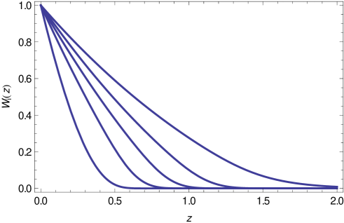
Figure 3.3: The window functions $W_{i}(z)$ for five redshift bins.

One of the most crucial functions being used in this calculation is the window function

$$W_{i}(z)=\int_{z}^{\infty}\frac{\,\mathrm{d}z^{\prime}}{H(z^{\prime})}\left(1-\frac{r(z)}{r(z^{\prime})}\right)n_{i}(r(z^{\prime})),$$ (3.60)

where $r(z)$ is the comoving distance at redshift $z$, i.e.

$$r(z)=\int_{0}^{z}\frac{\,\mathrm{d}z^{\prime}}{H(z^{\prime})}\,.$$ (3.61)

Lastly, we need the matter power spectrum $P_{m}$ to infer the convergence power spectrum. For this we use the fitting formulae covered in section 3.2.

3.4 Survey parameters

The quality of any weak lensing survey is determined by a set of parameters that includes the fraction of the sky covered, the median redshift, and so on. In table 3.1 all of the parameters that are used in our simulation are shown. Weak lensing surveys should aim at wide and deep field coverage. Since these projects are all still in development, the exact numbers that will be used in the end may vary, and some are still undecided.

Parameter	Value	Comment
$f_{\mathrm{sky}}$	0.5	Fraction of sky surveyed
$z_{m}$	0.9	Median redshift
$\Delta_{z}$	0.05	Relative photometric redshift error
$n_{\vartheta}$	35	Galaxy density per $\,\mathrm{arcmin}^{2}$
$\gamma_{\mathrm{int}}$	0.22	Intrinsic shear

Table 3.1: Shown here are typical values of survey parameters determining the quality of the experiment, which we will use in our calculation (cf. Huterer et al., 2006).

3.4.1 Ground based surveys: LSST

The Large Synoptic Survey Telescope, funded partially privately and by the U.S. Department of Energy, is a wide field survey telescope working in the visible band, located on the Cerro Pachón in Chile. It is currently in the design and development stage and is scheduled to be fully operational by 2020 with a lifetime of at least ten years. It will feature a 3.2 Gigapixel camera and a large aperture with an 8.4m (6.5m effective) primary mirror and cover the entire extra galactic sky of 20 000 deg² with a depth up to an apparent magnitude of $r\sim 27.7$ for point sources. Besides weak lensing measurements, the mission will observe super novae as well as map the Milky Way and small objects in the solar system (such as asteroids). This ultra wide and deep survey will provide a good data source for weak lensing observations.

3.4.2 Space based surveys: Euclid, WFIRST

Euclid is a proposed mission from ESA for a satellite orbiting the second Lagrangian point as part of their cosmic vision program. It is still in the definition phase and currently competing with PLATO and Solar Orbiter to be one the two missions that will be approved by ESA in mid 2011. It is foreseen to be launched in 2017 with a nominal mission lifetime of five years. This survey might also cover up to 20 000 deg². The telescope will be a 1.2m Korsch operating within the visible and infrared wavelengths with the ability of detecting galaxies in the redshift range $0.5<z<2$ and therefore provide an excellent probe for dark energy.

The Wide Field Infrared Survey Telescope (WFIRST, formerly known as JDEM-Omega) is another survey investigating dark energy, funded by NASA and the U.S. Department of Energy and proposed by the Joint Dark Energy Mission. In addition to weak lensing and baryon acoustic oscillations, WFIRST will also probe supernovae with high precision. It is still at a very early stage and has been postponed to launch at an unknown date, possibly not before 2025, due to budgeting and scheduling issues on a seperate project, the James Webb Space Telescope (Overbye, Jan 4, 2011).

Survey	$f_{\mathrm{sky}}$	$\Delta_{z}$	$z_{m}$	$n_{\vartheta}/\,\mathrm{arcmin}^{-2}$	Reference
LSST	$0.37$	0.02	$0.7$	$30$	Huterer et al. (2006); Ivezic et al. (2008)
Euclid	0.5	$0.05$	0.8	30-40	Laureijs (2009)
WFIRST	$0.25$	0.04	?	$\geq 30$	Gehrels (2010)

Table 3.2: Overview of current and planned surveys.

3.5 Fiducial model

In order to apply the Fisher matrix formalism, we need a fiducial cosmological model which represents the vector in parameter space where the likelihood has its maximum. We use the standard model of cosmology, a flat universe with cold dark matter and a cosmological constant (called $\Lambda$CDM, which makes six parameters). We additionally consider some extra parameters which are allowed to vary in a non-standard way, in particular

$$\bm{\theta}=(\omega_{m},\omega_{b},\tau,n_{s},\Omega_{m},w_{0},w_{1},\gamma,\Sigma_{0},\sigma_{8})\,,$$ (3.62)

where $\omega_{m}=\Omega_{m}h^{2}$ is the reduced fractional matter density, and $\omega_{b}$ is defined analogous for baryons. Their numerical values according to the WMAP 7-year data (Komatsu et al., 2010) can be seen in table 3.3. The growth index $\gamma$ is taken to be $6/11\approx 0.55$ in the standard model (Wang and Steinhardt, 1998).

It should be pointed out that the reionization optical depth $\tau$ is merely a remnant, and none of the functions in the code in later section depend on $\tau$; however, it was not removed, however, due to the possibility of future modifications to the code. The inclusion of functions that depend on $\tau$ will thus be easier, as long as we remember to cross out the according row and column in the resulting Fisher matrix.

Parameter	Fiducial value	Description
$\omega_{m}$	$0.1352(36)$	Reduced matter density today
$\omega_{b}$	$0.02255(54)$	Reduced baryon density today
$\Omega_{m}$	$0.275(11)$	Matter density today
$\tau$	$0.088(14)$	Reionization optical depth
$n_{s}$	$0.968(12)$	Scalar spectral index
$\sigma_{8}$	$0.816(24)$	Fluctuation amplitude at $8\,\mathrm{Mpc}/h$
$w_{0}^{\dagger}$	$-1$	Current equation-of-state ratio
$w_{1}^{\dagger}$	$0$	Higher order equation-of-state ratio
$\gamma^{\dagger}$	$6/11$	Growth index
$\Sigma_{0}^{\dagger}$	$0$	Parameterized Post-Newtonian parameter

Table 3.3: Our ten-parameter fiducial model. The second column represents the WMAP7+BAO+$H_{0}$ Mean taken from Komatsu et al. (2010). Quantities with a dagger are fixed in the standard flat $\Lambda$CDM model and thus not included here by the WMAP measurement. Uncertainties in the last two digits are given in parenthesis. They will be needed in Section 4.5.

3.6 Model-independent parameterization

3.6.1 Expansion rate

In order to see how observations can constrain the history of the expansion rate without assuming a particular parameterization of it, we take the values of the Hubble parameter at a series of redshifts determined in section 3.1 using our fiducial model and build a linearly interpolated function going through these supporting points. For this, we define

$$h_{i}=\ln H(\hat{z}_{i}),$$ (3.63)

where $\hat{z}_{i}$ is at the center of the $i$-th redshift bin. The use of the logarithm is purely for convenience. The Hubble parameter itself from now on is a linearly interpolated function through these points. It is evident that the dependency of the Hubble parameter on the other cosmological quantities changes from $H(z;\Omega_{m},w_{0},w_{1})$ to $H(z;h_{1},\ldots,h_{\mathcal{N}})$. The consequence of this is that all cosmological functions that depend on $H(z)$ are now treated as functions of the $h_{i}$s, resulting in $\mathcal{N}$ additional parameters being added to the fiducial model.

3.6.2 Growth function

The growth function is defined by

$$G(a)\equiv\frac{\Phi(a)}{\Phi(a_{T})}\,,$$ (3.64)

where $\Phi$ is the scalar gravitational potential from (2.8) and $a_{T}$ stands for the transfer epoch, which typically has a value of $0.03$ (see for instance A&T or Dodelson (2003)). Be advised that in relevant literature the growth function is often defined such that $G(a)$ needs to be replaced with $aG(a)$ in eq. (3.64). Also, it is sometimes referred to as $D$ or $D_{1}$. The growth function can be identified with the matter density contrast over the scale factor, i.e.

$$G(a)=\frac{\delta_{m}(a)}{a\delta_{m}(0)}\,,$$ (3.65)

which is given by

$$\delta_{m}(a)\equiv\frac{\rho(a)}{\langle\rho\rangle}-1\,.$$ (3.66)

A practical quantity in cosmology is the so called growth index $\gamma$, defined by

$$f(a)\equiv\Omega_{m}(a)^{\gamma}\,,$$ (3.67)

where $f$ is the growth rate

$$f(a)\equiv\frac{\,\mathrm{d}\ln\delta_{m}(a)}{\,\mathrm{d}\ln a}\,.$$ (3.68)

Note that the power law in eq. (3.67) is an empirically found fit for the growth rate (Wang and Steinhardt, 1998), which was shown to be accurate to within 0.2% of the exact solution (Linder, 2005).

After reminding ourselves that

$$\,\mathrm{d}\ln a=\frac{\,\mathrm{d}a}{a}=(1+z)\,\mathrm{d}\left(\frac{1}{1+z}\right)=-\frac{\,\mathrm{d}z}{1+z}\,,$$ (3.69)

we can eliminate $\delta_{m}(a)$ and $f$ from eqs. (3.64 - 3.67) to find

$$G(z)=G_{0}\exp\left({-\int_{0}^{z}\frac{\Omega_{m}(z^{\prime})^{\gamma}-1}{1+z^{\prime}}\,\mathrm{d}z^{\prime}}\right)\,,$$ (3.70)

where the matter density is

$$\Omega_{m}(z)=\frac{\rho_{m}(z)}{\rho_{m}(z)+\rho_{\Lambda}}=\frac{\Omega_{m}\times(1+z)^{3}}{E(z)}\,.$$ (3.71)

The only point where the growth function enters the calculation is via the matter power spectrum, which is given by (see A&T, p. 75; cf. eq. (3.8))

$$P_{m}(k,z)=\frac{2\pi^{2}\delta^{2}_{H}}{\Omega_{m}^{2}}\left(\frac{k}{H_{0}}\right)^{n_{s}}T(k)^{2}\frac{G(z)^{2}}{(1+z)^{2}}H_{0}^{-3}.$$ (3.72)

Just as in section 3.6.1 we can now finally define

$$g_{i}\equiv\ln G(\hat{z}_{i})$$ (3.73)

and replace the original growth function with a linear interpolation through the $\hat{z}_{i}$s. The number of parameters in our model thus increases to $10+2\mathcal{N}$. Naturally, every function that depends on the matter power spectrum now also becomes a function of the $g_{i}$s.

3.7 The figure of merit

In order to have a quantifiable gauge of the information content of the final result, we define the figure of merit (FOM) for the error bars on the $h_{i}$s and $g_{i}$s, respectively, as

$$\mathop{\mathrm{FOM}}(H)\equiv \sum_{i=1}^{\mathcal{N}}\sigma(h_{i})^{-2}\,,$$ (3.74)

$$\mathop{\mathrm{FOM}}(G)\equiv \sum_{i=1}^{\mathcal{N}}\sigma(g_{i})^{-2}\,.$$ (3.75)

It is obvious that the smaller the error bars are, the larger the FOM becomes. The idea of using this definition is that the FOM should not change too much if only one error bar is significantly larger than all the other ones.

While the particular value of the FOM has no deeper meaning, it provides a convenient tool to easily compare the errors resulting from different sets of parameters. Note that this definition does not match the popular definition by the Dark Energy Task Force, which suits a different purpose (Albrecht et al., 2006).

3.8 An implementation in Mathematica 

To do the actual computation, we use Mathematica 8.0.1.0, which supplies us with all necessary numerical procedures.

In an attempt to seperate all the parameters that determine the final outcome of the computation from the rest of the code, they are all defined at the beginning of the Mathematica notebook. We further calculate a checksum, a digital fingerprint of those parameters via an injective map from the set of all parameters onto the set of integers, comparable to a hash function. This will be useful when we store results in a file when changing the parameters without having to worry about overwriting previous results. We can roughly differentiate between physical parameters (such as matter density, baryon density, etc.) and technical parameters (the limit of a certain integral, step size in an interpolating function, etc.). For an overview, we refer to tables 3.4, 3.5, and 3.6.

Functions
logprint[string]	Prints messages and saves them to a log file
loadfile[filename]	Uses pre-calculated expressions if applicaple
ngal[[i]][z]	$n_{i}(z)$
hub[z,dbins]	$H(z;h_{1},\dots,h_{\mathcal{N}})$
dist[z,dbins]	$r(z)$
omgen[z,om,w0,w1]	$\Omega_{m}(z)$
growthfastgen[z,gbins]	$G(z;g_{1},\dots,g_{\mathcal{N}})$
wind[i,z,om,dbins]	$W_{i}(z)$
pk[k,z,...]	$P_{m}(k)$ (Linear)
pknl[k,z,...]	$P_{m}(k)$ (Non-linear)
clnngen[i,j,ell,...]	$P_{ij}(\ell)$
dcdp[pi,i,j,ell,ref]	$\partial P_{ij}/\partial\theta_{pi}$

Table 3.4: Functions as used in the Mathematica notebook.

Physical parameters
omh2	$\omega_{m}$	obh2	$\omega_{b}$
tau	$\tau$	ns	$n_{s}$
om	$\Omega_{m}$	w0	$w_{0}$
w1	$w_{1}$	gamma	$\gamma$
gppn	$\Sigma_{0}$	s8	$\sigma_{8}$
dbins[[i]]	$h_{i}$	gbins[[i]]	$g_{i}$

Table 3.5: Variables referring to physical parameters as used for arguments in functions in the Mathematica notebook. Their fiducial value is stored in a variable that has the string ref attached.

Technical parameters
zlimit	3	Redshift limit after which we assume $n(z)\approx 0$
nbins	5	Number of redshift bins $\mathcal{N}$
eps	0.025	Step size for numerical differentiation
zsigma	4	Integration length in units of standard deviations
zsmax	4	Maximum redshift for interpolated functions
fitstepz	0.2	Step size for interpolated functions
lellmax	4	Decadic logarithm of upper limit of the multipole
lellmin	2	Decadic logarithm of lower limit of the multipole
lstep	0.2	Decadic logarithmic step size of the multipole
piv		List of parameters that are not fixed
dir		Directory where data is stored

Table 3.6: Parameters determining the accuracy of the result and their default value.

In the first section of actual computation, we infer the boundaries of the redshift bins depending only on $\mathcal{N}$, $\Delta_{z}$, and the galaxy distribution function $n(z)$. The definition of the necessary cosmological functions is straight forward. They often involve the computation of time intensive numerical integrals, especially the highly used window function. These functions are interpolated by cubic splines. All functions are sufficiently “nice” (not more than one extremum) so that we do not have to retreat to more conservative linear splines.

In order to save processing time and memory (especially in sequenced executions of the notebook) we employ a little trick when computing expensive functions. To avoid loss of data after unexpected computer crashes, it makes sense to store not only the final result, i.e. the Fisher matrix, but also intermediate results on the hard drive. For this, the function loadfile evaluates the expression given in the second argument only if the file given in the first argument does not exist, and then stores the result in said file and returns it. If the file does exist, the expression in it will be loaded and returned. This is applied to all time sensitive functions. All files are saved in dir, which contains the checksum of all parameters, except for the window functions $W_{i}(z)$. Because they only depend on $\Omega_{m}$, $\mathcal{N}$, the $h_{i}$s and the number of the redshift bin, they are stored in a sibling directory to save computing time when calculating the Fisher matrix after only, say, $\Delta\lg\ell$ has changed. The computation of the interpolating functions of the window functions has also been parallelized by using the Mathematica command ParallelTable.

Very often we have to interpolate a function depending on several parameters, such as the window function $W_{i}(z;\Omega_{m},h_{1},\dots h_{\mathcal{N}})$, which generally needs to be evaluated for the derivatives at all $0<z<3$ for $\Omega_{m}$, $\Omega_{m}(1\pm\epsilon)$ and so on. We define the function such that it is computed only when needed, which can be achieved in Mathematica by writing schematically

fAux[a_] := fAux[a] =
    Interpolation[Table[{x,f[x,a]},{x,x0,x1,dx}]];
fFast[x,a] := fAux[a][x];

The fFast[x,a] is a fast, interpolated version of f[x,a], where x is the variable and a a parameter. The extra = sign in the first line makes Mathematica look up the cached value if there is one, preventing it from making an expensive computation more than once.

What follows is a relatively straight forward implementation of sections 3.2 and 3.3. It is important to note, however, that all the functions that ultimately depend on the growth function, i.e. all functions that depend on the linear matter power spectrum, have been overloaded such that they might take gbins as an argument, in which case the power spectrum uses the interpolated growth function. The reason for this will become apparent in chapter 4.

Most functions have been carefully defined to avoid warnings by Mathematica concerning numerical issues like non-converging integrals. Vanishing integrals are hard to detect with numerical methods, since a sufficiently sharp, high peak would require an arbitrary large number of sampling points. Many functions have been tweaked (if possible) to avoid these warnings. Very often, Mathematica also tries to simplify an expression before plugging in actual values, which causes a lot of warnings and can slow down the computation significantly. To prevent this, we declared certain arguments as “numerical” so that Mathematica plugs in these values immediately. For instance the comoving distance is defined as

    dist[z_?NumericQ, dbins_] := NIntegrate[1/hub[zx, dbins],
        {zx, 0, z}];

This way, Mathematica will not try to numerically evaluate the integral in a subsequent definition of a function (which would be futile) before a specific value for the redshift is given. We found that this significantly reduces numerical instabilities and improves the overall results.

Chapter 4 Results

Before we cover the analysis of the results, it needs to be pointed out that two Fisher matrices have been calculated. The first Fisher matrix was computed while using the standard expression in eq. (3.70) for $G(z)$ and linearly interpolating $H(z)$, and the second Fisher matrix was computed by linearly interpolating both $H(z)$ and $G(z)$. We will refer to this as the $H$-case and the $G$-case respectively. This introduces a certain degeneracy, since the variables $h_{i}$ occur in both the $H$-case and the $G$-case and generally take on different values. Hence we will denote those variables in the $H$-case as $\hat{h}_{i}$ to avoid confusion, although they will be barely used.

Unless mentioned otherwise, the Fisher matrix has been calculated using the parameters shown in tab. 3.6, where we cross out the rows and columns corresponding to $(\tau,w_{0},w_{1},\gamma,\Sigma_{0})$ in the standard case. The order of our parameters was given in eq. (3.62); here is a reminder:

$$\bm{\theta}=(\omega_{m},\omega_{b},\tau,n_{s},\Omega_{m},w_{0},w_{1},\gamma,\Sigma_{0},\sigma_{8})\,.$$ (4.1)

From the resulting Fisher matrix, we can easily extract the errors on each cosmological parameter. A typical example of plotting the error bars on the Hubble parameter and growth function can be seen in fig. 4.1.

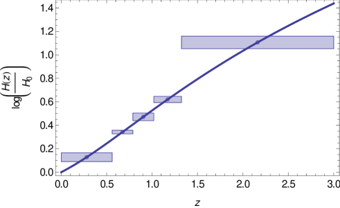
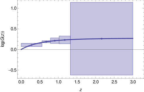
Figure 4.1: A typical plot of the error bars on the $h_{i}$s (top) and $g_{i}$s (bottom) for $\mathcal{N}=5$ with a figure of merit of 7634 and 2865 respectively. The bins are chosen such that they all contain the same number of galaxies.

4.1 Consistency checks

Since we naturally cannot compare our results with observations within the next decade, we have limited means to make sure that they are meaningful and error free. One way to check is to see whether the matrix satisfies basic properties, another is to compute intermediate, partial results and compare them with the numerical results. A first approach would be to visually compare the derivative of the convergence power spectrum in two particular bins with respect to a particular cosmological parameter, e.g.

$$\frac{\partial P_{12}(\ell)}{\partial g_{1}}\,,$$ (4.2)

with and without interpolated functions. However, this turned out to be unpractical due to the long runtime of over three days even with the use of four parallel kernels and reducing the sampling points in the numerical integration down to 50.

But we can still easily do another check. As the negative of the Hessian of a function at its maximum, the Fisher matrix needs to be positive definite. Looking at the eigenvalues of the Fisher matrix, we find in the $H$-case (descending order)

$$\bm{\lambda}_{H}=(1.03\times 10^{8},4.87\times 10^{6},1.89\times 10^{5},7.29\times 10^{4},3.34\times 10^{4},\\ 9.11\times 10^{3},6.71\times 10^{3},6.57\times 10^{2},3.2\times 10^{2},1.06\times 10^{2},\\ 4.76\times 10^{1},1.67\times 10^{1},3.53,1.04\times 10^{-2},1.4\times 10^{-15})\,.$$ (4.3)

Note that the last eigenvalue is thirteen orders of magnitude smaller than the next largest eigenvalue. The corresponding normalized eigenvector is, while neglecting numbers that are smaller than $10^{-13}$,

$$\bm{e}_{H,15}=(0,0,-1.0,0,0,0,0,0,0,0,0,0,0,0,0)\,.$$ (4.4)

This reveals that it points only in the $\tau$-direction in parameter space, as we can see in eq. (4.1). This degeneracy is expected, since the convergence power spectrum does not depend on $\tau$. All other eigenvalues are positive, so this check is passed.

In the $G$-case, the eigenvalues of the Fisher matrix are

$$\bm{\lambda}_{G}=(1.24\times 10^{8},5.21\times 10^{6},6.63\times 10^{5},1.86\times 10^{5},8.85\times 10^{4},\\ 4.08\times 10^{4},9.26\times 10^{3},7.65\times 10^{3},2.96\times 10^{3},1.\times 10^{3},\\ 5.16\times 10^{2},1.4\times 10^{2},30.3,7.36,3.56,0.83,\\ -1.92\times 10^{-14},5.33\times 10^{-15},-5.31\times 10^{-15},1.07\times 10^{-46})\,.$$ (4.5)

There are two negative eigenvalues among the last four of them, but as they are at least thirteen orders of magnitude smaller than the next largest eigenvalue, they are consistent with zero. Again, analyzing the according eigenvectors while neglecting values below $10^{-13}$ yields

$$\bm{e}_{G,17} =(0,0,0,0,0,0.085,-0.23,0.97,0,0,0,0,0,0,0,0,0,0,0,0)$$ (4.6)

$$\bm{e}_{G,18} =(0,0,0,0,0,0.98,0.17,-0.047,0,0,0,0,0,0,0,0,0,0,0,0)$$ (4.7)

$$\bm{e}_{G,19} =(0,0,0,0,0,-0.15,0.96,0.24,0,0,0,0,0,0,0,0,0,0,0,0)$$ (4.8)

$$\bm{e}_{G,20} =(0,0,1.0,0,0,0,0,0,0,0,0,0,0,0,0,0,0,0,0,0)\,.$$ (4.9)

Comparing again with eq. (4.1) shows that these eigenvectors lie in the parameter subspace spanned by $\tau$, $w_{0}$, $w_{1}$ and $\gamma$, as we would expect since now the growth function depends on the $g_{i}$s instead of the equation-of-state parameters $w_{i}$ and the growth index $\gamma$. At this point, the convergence power spectrum does not depend on any quantity that in turn depends on those parameters, so the Fisher matrix will be degenerate if we do not cross out the according rows and columns. Just like in the $H$-case, all remaining eigenvalues are positive.

4.2 Improving the figure of merit

In this section we want to find out how the FOM behaves when we modify various parameters. This provides us with a way of gauging the quality of the tomography process, seeing how much information we were able to extract out of the weak lensing signal.

4.2.1 Impact of the number of redshift bins

Running the Mathematica notebook for various values of $\mathcal{N}$ lets us compare the FOM for different binning. To get optimal results, we let the number of redshift bins $\mathcal{N}$ run between 2 and 20, using the values 2, 3, …, 10, 15 and 20. In fig. 4.2, we can clearly see a peak at $\mathcal{N}=3$ in the $H$-case with a decreasing trend for higher numbers of redshift bins.

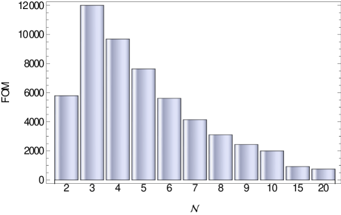
Figure 4.2: Comparing the FOM for various values of $\mathcal{N}$ in the $H$-case.

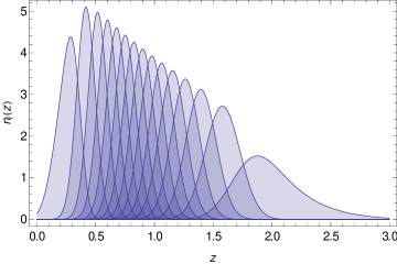
Figure 4.3: The galaxy distribution function in 15 redshift bins, which are overlapping heavily.

Doing the same in the $G$-case yields a slightly different result, shown in fig. 4.4. Here the FOM for $H$ peaks at $\mathcal{N}=6$ while the FOM for $G$ peaks at $\mathcal{N}=3$.

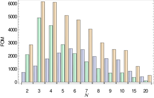
Figure 4.4: In the $G$-case, the FOM in dependence of $\mathcal{N}$ takes a slightly different shape. Blue represents $\mathop{\mathrm{FOM}}(H)$, green is $\mathop{\mathrm{FOM}}(G)$ and yellow is the sum of both.

When examining the galaxy distribution function for each bin (see fig. 4.3) in the case of 15 redshift bins, we can see that with our assumed photometric redshift error they are “smeared out” to the point where it becomes impossible to confidently assign a redshift bin to a given galaxy.

4.2.2 On $\ell_{\mathrm{max}}$ and $\Delta{\lg\ell}$

It is not obvious how far the sum in eq. (3.51) should go or what the step size for $\ell$ should be. Estimating a realistic value for the upper limit $\ell_{\mathrm{max}}$ has been done in eq. (3.7), but it is interesting to see how the FOM behaves for larger values. We therefore try several values for $\ell_{\mathrm{max}}$ and see whether the FOM approaches some constant or not. The result can be seen in fig. 4.5.

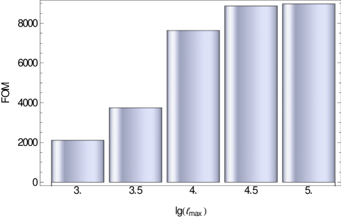
Figure 4.5: When increasing $\ell_{\mathrm{max}}$, the upper limit of the sum in eq. (3.51), the FOM changes, but increases by less than 15% beyond $\ell_{\mathrm{max}}=10^{4}$. Shown here is the $H$-case, the $G$-case looks similar.

We observe that the FOM only changes slightly for values above 4, as we would expect due to the finite angular galaxy density.

Doing the same for some values for $\Delta{\lg\ell}$ at a fixed $\ell_{\mathrm{max}}=10^{4}$ yields the numbers used in fig. 4.6. We see that essentially all the information is being extracted at a logarithmic multipole step size of $0.2$. This figure roughly matches the result of $0.3$ found in Bernstein (2009), where it is argued that the broad window function “smoothes away fine structure” in the convergence power spectrum, such that at some point further increasing of the number of multipole bins will no longer have beneficial effects. On the other hand, it is interesting to note that the FOM increases almost by an order of magnitude by going from $\Delta\lg\ell=0.8$ to $0.4$.

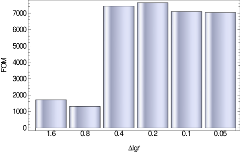
Figure 4.6: The figure of merit for various values of $\Delta{\lg\ell}$ in the $H$-case. Going beyond $0.2$ does not change much. The situation is the same in the $G$-case and thus not shown here.

4.3 Fixing various parameters

In order to determine the parameter which the Fisher matrix is most sensitive, we will fix one additional parameter after another and analyze the behavior of the FOM. Remember, fixing a parameter within the Fisher matrix formalism is as easy as crossing out the according row and column of the Fisher matrix. As we can see in fig. 4.7, knowing the scalar spectral index $n_{s}$ in the $H$-case as well as possible pays off the most, as the FOM increases roughly by a factor of three if we know it exactly.

On the other hand, in the $G$-case, depicted in fig. 4.8, it is most beneficial to know $\Omega_{m}$ (factor of six) to get the highest increase in $\mathop{\mathrm{FOM}}(H)$, but knowing $\sigma_{8}$ exactly gives another factor of two for $\mathop{\mathrm{FOM}}(G)$.

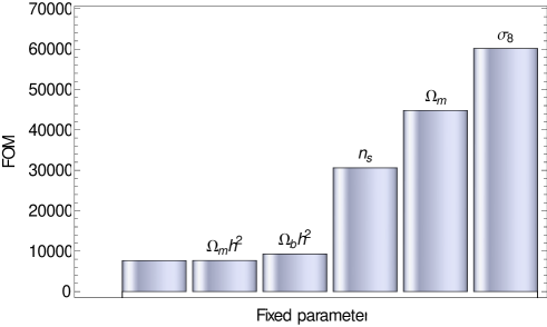
Figure 4.7: Various parameters are being fixed successively ($H$-case). Each bar is labeled with the parameter that has been fixed on top of the previous one, such that all of them are fixed on the right side of the diagram. Fixing the scalar spectral index is most beneficial, as the FOM triples in the best case.

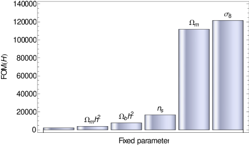
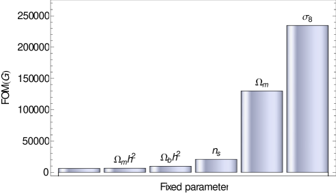
Figure 4.8: Various parameters are, again, being fixed successively ($G$-case). Here, knowledge about $\Omega_{m}$ and $\sigma_{8}$ pays off most for $\mathop{\mathrm{FOM}}(H)$ (top) and $\mathop{\mathrm{FOM}}(G)$ (bottom) respectively.

4.4 Uncertainties

Finally, we can present the uncertainties on the values of $H$ and $G$ at different redshifts. We use the parameters $\mathcal{N}=5$, $\ell_{\mathrm{max}}=10^{4}$ and $\Delta{\lg\ell}=0.2$ and find the results shown in tables 4.1 and 4.2. These are derived from the full Fisher matrix as seen in tab. 4.3 (for the $G$-case). As expected, the constraints in the $G$-case are not as tight as those in the $H$-case, since we allow the growth function to vary in a more general way.

	$\sigma(\omega_{m})$	$\sigma(\omega_{b})$	$\sigma(n_{s})$	$\sigma(\Omega_{m})$	$\sigma(\sigma_{8})$
$H$-case	0.17	0.065	0.049	0.012	0.011
$G$-case	0.17	0.066	0.059	0.021	0.041

$i$	1	2	3	4	5
$\sigma(\hat{h}_{i})$	0.038	0.015	0.033	0.026	0.053
$\sigma(h_{i})$	0.044	0.036	0.044	0.049	0.48
$\sigma(g_{i})$	0.039	0.023	0.068	0.094	0.88

Table 4.1: Errors on the cosmological parameters as well as $\hat{h}_{i},h_{i},g_{i}$ while fixing $\tau,w_{0},w_{1},\Sigma_{0},\gamma$ and keeping $\mathcal{N}=5$, $\ell_{\mathrm{max}}=10^{4}$, $\Delta{\lg\ell}=0.2$.

$\sigma(\omega_{m})$	$\sigma(\omega_{b})$	$\sigma(n_{s})$	$\sigma(\Omega_{m})$	$\sigma(w_{0})$	$\sigma(w_{1})$	$\sigma(\gamma)$	$\sigma(\Sigma_{0})$	$\sigma(\sigma_{8})$
0.23	0.081	0.077	0.045	3.0	9.3	0.67	0.40	0.11

Table 4.2: Errors on the cosmological parameters while fixing $\tau$, marginalizing everything else, and keeping $\mathcal{N}=5$, $\ell_{\mathrm{max}}=10^{4}$, $\Delta{\lg\ell}=0.2$ in the $H$-case.

$\Omega_{m}h^{2}$	$\Omega_{b}h^{2}$	$n_{s}$	$\Omega_{m}$	$\sigma_{8}$	$h_{1}$
5.89991e6	-1.29794e7	3.04031e6	1.77766e7	8.47979e6	-3.10712e6
-1.29794e7	2.85559e7	-6.68462e6	-3.91594e7	-1.86837e7	6.8399e6
3.04031e6	-6.68462e6	1.57342e6	9.0384e6	4.30423e6	-1.59096e6
1.77766e7	-3.91594e7	9.0384e6	6.56348e7	3.13299e7	-1.06167e7
8.47979e6	-1.86837e7	4.30423e6	3.13299e7	1.50269e7	-5.05321e6
-3.10712e6	6.8399e6	-1.59096e6	-1.06167e7	-5.05321e6	1.99529e6	…
-1.94576e6	4.28365e6	-9.92991e5	-7.29185e6	-3.45161e6	9.6474e5
-1.16652e5	2.56784e5	-5.94073e4	-4.72584e5	-2.22597e5	4.63944e4
4.1346e6	-9.11132e6	2.09669e6	1.51661e7	7.2877e6	-2.56814e6
1.91022e6	-4.20561e6	9.75038e5	6.89405e6	3.2877e6	-9.21068e5
4.52229e4	-9.9446e4	2.3215e4	1.77003e5	8.31533e4	-1.48989e4

	$h_{2}$	$h_{3}$	$g_{1}$	$g_{2}$	$g_{3}$
	-1.94576e6	-1.16652e5	4.1346e6	1.91022e6	4.52229e4
	4.28365e6	2.56784e5	-9.11132e6	-4.20561e6	-9.9446e4
	-9.92991e5	-5.94073e4	2.09669e6	9.75038e5	2.3215e4
	-7.29185e6	-4.72584e5	1.51661e7	6.89405e6	1.77003e5
	-3.45161e6	-2.22597e5	7.2877e6	3.2877e6	8.31533e4
…	9.6474e5	4.63944e4	-2.56814e6	-9.21068e5	-1.48989e4
	1.03799e6	7.90972e4	-1.55933e6	-9.6674e5	-3.22527e4
	7.90972e4	7.59839e3	-9.07882e4	-7.37654e4	-3.24212e3
	-1.55933e6	-9.07882e4	3.61394e6	1.48555e6	3.17958e4
	-9.6674e5	-7.37654e4	1.48555e6	9.18941e5	3.03478e4
	-3.22527e4	-3.24212e3	3.17958e4	3.03478e4	1.4814e3

Table 4.3: The full Fisher matrix in the $G$-case for three redshift bins.

4.5 Including priors

As mentioned in section 2.4.1, the magic of Fisher lets us easily include priors from other experiments. All we need to do is line up the right rows and columns of two different Fisher matrices and take their sum, i.e.

$$F_{ij}^{\prime}=F_{ij}+F_{ij}^{\mathrm{prior}}.$$ (4.10)

We can do this for two measurements of the cosmic microwave background radiation. The first one is an already completed experiment, namely WMAP, and the second one a planned mission, Planck, both of which use the same fiducial model as in this thesis.

4.5.1 WMAP

A Gaussian prior, that is a fiducial value $p_{i}$ with Gaussian error $\sigma(p_{i})$, is represented simply by a Fisher matrix that has $\sigma(p_{i})^{-2}$ as its $i$-th diagonal entry (Albrecht et al., 2006). Gaussian priors can be obtained from recent observations. We use the data from the WMAP survey, one of the most precise measurements of cosmological parameters as of now. The standard deviations can be taken from table 3.3 and—while taking into consideration the order we are using—the corresponding Fisher matrix thus becomes

$$\mathbf{\mathsf{F}}^{\mathrm{WMAP7}}=\mathrm{diag}\, [77160.5,3.42936\text{e6},5102.04,$$

$$6944.44,9291.96,0,0,0,0,1736.11,0,\dots,0]\,.$$ (4.11)

4.5.2 Planck

The Fisher matrix $\hat{\mathbf{\mathsf{F}}}^{\mathrm{Planck}}$ for the planned Planck mission is shown in table 4.4.

	$w_{0}$	$w_{a}$	$\Omega_{\mathrm{DE}}$
$w_{0}$	.172276e+06	.490320e+05	.674392e+06
$w_{a}$	.490320e+05	.139551e+05	.191940e+06
$\Omega_{\mathrm{DE}}$	.674392e+06	.191940e+06	.263997e+07
$\Omega_{k}$	$-$.208974e+07	$-$.594767e+06	$-$.818048e+07	…
$\omega_{m}$	.325219e+07	.925615e+06	.127310e+08
$\omega_{b}$	$-$.790504e+07	$-$.224987e+07	$-$.309450e+08
$n_{S}$	$-$.549427e+05	$-$.156374e+05	$-$.215078e+06

	$\Omega_{k}$	$\omega_{m}$	$\omega_{b}$	$n_{S}$
	$-$.208974e+07	.325219e+07	$-$.790504e+07	$-$.549427e+05
	$-$.594767e+06	.925615e+06	$-$.224987e+07	$-$.156374e+05
	$-$.818048e+07	.127310e+08	-.309450e+08	$-$.215078e+06
…	.253489e+08	$-$.394501e+08	.958892e+08	.666335e+06
	$-$.394501e+08	.633564e+08	$-$.147973e+09	$-$.501247e+06
	.958892e+08	$-$.147973e+09	.405079e+09	.219009e+07
	.666335e+06	$-$.501247e+06	.219009e+07	.242767e+06

Table 4.4: Fisher matrix $\hat{\mathbf{\mathsf{F}}}^{\mathrm{Planck}}$ for ($w_{0}$, $w_{a}$, $\Omega_{\mathrm{DE}}$, $\Omega_{k}$, $\omega_{m}$, $\omega_{b}$, $n_{s}$) derived from the covariance matrix for $(R,l_{a},\Omega_{b}h^{2},n_{s})$ from Planck (Mukherjee et al., 2008).

This matrix needs to be transformed for compatibility with our Fisher matrix. The parameter transformation is given by

$$\bm{\theta}^{\prime}(\bm{\theta})=(\theta_{5},\theta_{6},\text{const.},\theta_{7},1-\theta_{3},\theta_{1},\theta_{2},\text{const.},\dots,\text{const})\,,$$ (4.12)

where $\bm{\theta}^{\prime}=(\omega_{m},\omega_{b},\tau,n_{s},\Omega_{m},w_{0},w_{1},\gamma,\Sigma_{0},\sigma_{8},h_{1},\dots,g_{1},\dots)$ is the vector in parameter space in our formalism, and $\bm{\theta}=(w_{0},w_{a},\Omega_{\mathrm{DE}},\Omega_{k},\omega_{m},\omega_{b},n_{s})$ is the vector in parameter space in the formalism of Mukherjee et al. (2008). The Jacobian matrix thus reads

$$J_{ij}=\left(\frac{\partial\theta^{\prime}_{i}}{\partial\theta_{j}}\right)^{T}=\underbrace{\left(\begin{array}[]{cccccccccc}0&0&0&0&0&1&0&0&\dots&0\\ 0&0&0&0&0&0&1&0&\dots&0\\ 0&0&0&0&-1&0&0&0&\dots&0\\ 0&0&0&0&0&0&0&0&\dots&0\\ 1&0&0&0&0&0&0&0&\dots&0\\ 0&1&0&0&0&0&0&0&\dots&0\\ 0&0&0&1&0&0&0&0&\dots&0\\ \end{array}\right)}_{10+\mathcal{N}(+\mathcal{N})\textrm{ columns}}\,.$$ (4.13)

The zeros on the right hand side account for the $\hat{h}_{i}$s (or $h_{i}$s and $g_{i}$s), which the original Planck Fisher matrix naturally does not contain. The Fisher matrix with the Planck prior for our use is then

$$\mathbf{\mathsf{F}}^{\mathrm{Planck}}=\mathbf{\mathsf{J}}^{T}\hat{\mathbf{\mathsf{F}}}^{\mathrm{Planck}}\mathbf{\mathsf{J}}.$$ (4.14)

4.5.3 Summary

We can now examine how including priors from WMAP, Planck, or both will affect the constraints on $H(z)$ or $G(z)$. For this, we will choose $\mathcal{N}=5$ while marginalizing over all other parameters, although $G(z)$ is fixed when calculating the $\mathop{\mathrm{FOM}}(H)$. The results are summarized in table 4.5.

	WL	WL+WMAP7	WL+Planck	WL+Planck+WMAP7
$\mathop{\mathrm{FOM}}(H)$	7636	13778	25194	26096
$\mathop{\mathrm{FOM}}(G)$	2865	5697	4350	6805

Table 4.5: Comparison of the FOM when including different priors for the $H$-case and the $G$-case, respectively.

Naturally, the FOM improves in both cases as we include additional priors. Unexpectedly, the growth function is more constrained by assuming WMAP priors compared to Planck priors. With Planck being one generation ahead of WMAP, it should be the other way around. But if we take fig. 4.8 into consideration, it is clear that while fixing $\Omega_{m}$ is most important for constraining $G$, fixing $\sigma_{8}$ also almost doubles the FOM. Unlike the WMAP prior, the Planck prior does not constrain $\sigma_{8}$ at all, thus even though Planck constrains $\Omega_{m}$ much more than WMAP in this parameter configuration, it is not as important with regard to constraining the growth function. Another observation we can make is that in either case the FOM does not increase significantly compared to the next higher value when including the second prior, i.e. the FOM in the $H$-case, when including WMAP and Planck, is almost the same as only including Planck. In the $G$-case, the FOM is almost the same when including both priors as compared to only including WMAP. This is to be expected, as both experiments probe the cosmic microwave background radiation, except with different sensitivities. Therefore, no more cosmological information can be extracted.

4.6 Comparison to current constraints

When we try to compare how weak lensing in this context will constrain the growth function compared to current constrains, we notice that our constraints are very poor at high redshifts. Rapetti et al. (2010) measured the growth index via a combination of X-ray cluster growth data with cluster gas mass fraction, type 1a supernovae, baryon acoustic oscillations and cosmic microwave background data, where they found that $\gamma=0.55^{+0.13}_{-0.10}$. As shown in fig. 4.9, these constraints are not very tight when applied to the growth function (even when assuming that $\Omega_{m}$ is known exactly), but the error bars from the Fisher matrix analysis hardly seem any better, especially at high redshifts. It is interesting, though, to have a model independent confirmation of our observations that is comparable with current constraints.

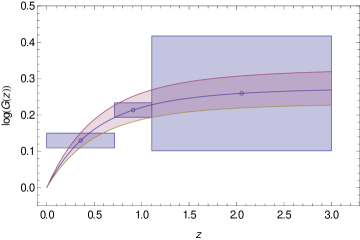
Figure 4.9: Current constraints on the growth function via the growth index by using X-ray cluster growth data. Shown is the $1\sigma$ confidence band of the growth funcion.

4.7 Possibility of ruling out modified gravity models

According to the data displayed in fig. 4.4, we get the best results for the growth function when using three redshift bins, which is why we shall adopt this number for this and the next section. Fig. 4.10 shows the error bars on $G(z)$ in this case, along with the growth function as predicted by the Starobinsky model with $\gamma_{\mathrm{Sta}}=0.42$ (Fu et al., 2010; Starobinsky, 2007) and the DGP model with $\gamma_{\mathrm{DGP}}$ by Dvali, Gabadadze and Porrati (Gong, 2008; Dvali et al., 2000). We also see the same diagram with priors from WMAP and Planck included. From the visual, we recognize a slight disagreement at low redshifts while the error bars at high redshifts are too large to make any statements about the competing models.

One caveat: The Starobinsky model actually predicts a redshift dependent growth index. Trying to fit a power law to the growth rate in this case, i.e. $f=\Omega_{m}(z)^{\gamma}_{\mathrm{Sta}}$ with a constant $\gamma_{Sta}$, yields a deviation of up to 10% at intermediate redshifts, which indicates that the result cited above is biased. A linear expression for the growth index, $\gamma_{\mathrm{Sta}}=\gamma_{0}+\gamma_{1}z$, is more accurate but fails at high redshifts with $z>0.5$. However, the result, $\gamma_{1}\approx-0.24$ indicates a decreasing growth index (Fu et al., 2010). Thus, in the case of the Starobinsky model the power law does not seem to be a good fit and the following discussion should be taken with a grain of salt.

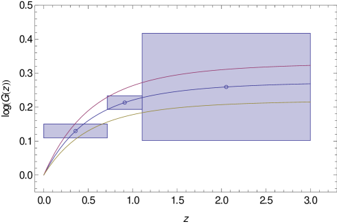
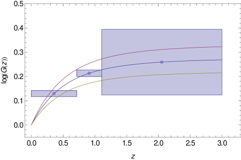
Figure 4.10: The growth function with error bars for the binning with the highest FOM. Also shown (from the top): The growth function from eq. (3.70) for the DGP model $\gamma_{\mathrm{DGP}}=11/16\approx 0.69$, the standard model $\gamma=6/11\approx 0.55$ and the Starobinsky model with $\gamma_{\mathrm{Sta}}=0.42$. Top panel: Weak lensing only. Bottom panel: Including priors from WMAP and Planck.

We now want to attempt to quantify the deviation from these two models. Assuming the errors on the growth function are Gaussian, we can compute the likelihood function for the growth index $\gamma$ as

$$\mathcal{L}(\gamma)=\exp\left(-\frac{1}{2}\sum_{i=1}^{3}\frac{(G(z_{i};\gamma)-g_{i})^{2}}{\sigma(g_{i})^{2}}\right)$$ (4.15)

using the error estimates from the Fisher matrix and keeping $\Omega_{m}$ fixed. The likelihood is plotted in fig. 4.11. Obviously, the maximum of the likelihood is found at the fiducial value $\gamma=0.55$. In this case, the likelihood can be approximated by a Gaussian with good agreement, and we find a standard deviation of $\sigma_{0}(\gamma)=0.056$ with weak lensing only and $\sigma_{1}(\gamma)=0.037$ while including priors from WMAP and Planck. Considering that both the DGP model as well as the Starobinsky model deviate from the fiducial value by at least $\Delta\gamma=0.13$, they could both be ruled out at the $2\sigma$ confidence level with weak lensing only and at the $3\sigma$ confidence level with priors. This does not seem to be entirely conclusive, especially when we consider the uncertainty in the $\gamma_{\mathrm{Sta}}$ that we mentioned earlier. However, we need to keep in mind that these constraints are model independent.

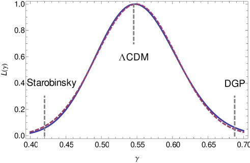
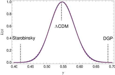
Figure 4.11: The likelihood for the growth index with a fitted Gaussian (dashed line). Indicated are the predicted values for the Starobinsky, DGP and standard model. Top panel: Weak lensing only. The Gaussian has a standard deviation of $\sigma=0.056$. Bottom panel: Including priors from WMAP and Planck. Here, the standard deviation is $\sigma=0.037$.

4.8 Problems and outlook

It is not surprising that the Fisher matrix formalism can only provide a lower bound on the expected error bars. This bound is called the Cramér-Rao bound, which expresses the fact that the maximum likelihood estimate constrains the model parameters at best with the value given by the Fisher matrix (Shao, 2003). We should also keep in mind that when the errors become too large, the approximation of the likelihood by a Gaussian may lose its validity.

Besides that, we did not take into account several systematic errors that might present itself while observing the weak lensing signal, like the aforementioned intrinsic alignment. Other potential error sources include: shear calibration errors, intrinsic galaxy alignment, and non-Gaussian statistics, some of which are discussed in Bernstein (2009) and Albrecht et al. (2009).

Regarding the source code of the notebook, while it does satisfy all the requirements for calculating the Fisher matrix, there certainly is still substantial room for improvement. One desirable feature would be the abstraction of cosmological parameters, such that they would not have to be hard coded into the arguments of any function, making it easier to add or remove parameters later on. In appendix A, large parts of the code were reused, but almost all arguments had to be adjusted manually, a cumbersome and error prone job. Another issue, that the runtime on a typical machine is of order several hours to a few days with parallelizing part of the code, which could perhaps be reduced significantly by examining the step size of interpolated functions more carefully. Many of them (and especially the window functions, a very central part of the computation) only have a single extremum and tend to approach zero after that. Limiting the evaluation of sampling points specifically to regions where the function takes non-negligible values might speed up the computation drastically. From a more structural point of view, a more modular setup by using Mathematica packages would be desirable to avoid duplicate code fragments, which would make the program more expandable, robust, and easier to use.

Chapter 5 Conclusion

We presented and developed the formal basis of the theory of dark energy, weak lensing, and statistics in cosmology (in particular the Fisher matrix formalism), on which the remainder of this thesis built. Furthermore, we described the specifics of the methods of weak lensing tomography using fitting formulas for the matter power spectrum with non-linear corrections and how it is used to compute the observable, the convergence power spectrum. It was demonstrated how we avoided assuming an underlying model for the Hubble parameter and growth function by using linear interpolation based on a choice of redshift bins. We showed how the convergence power spectrum is related to the matter power spectrum and how the matter power spectrum can be separated into the growth function and the transfer function. We gave the fitting formula for the transfer function and how the non-linear corrections are applied. Finally, we outlined how to implement the computation in Mathematica and what kind of challenges might arise in doing so.

Then we analyzed the behavior of the Fisher matrix when varying different parameters and why it makes sense to use their particular values. We showed how to include priors from other experiments and how it improves the FOM, a quantity that we defined as a quality measure. We found that a small number number of redshift bins is sufficient to extract most of the cosmological information from the weak lensing signal – five for best constraints of $H(z)$ and three for $G(z)$. It turned out that the error bars on the growth function are most sensitive to the fractional matter density $\Omega_{m}$ and power spectrum amplitude $\sigma_{8}$. The results indicated that the constraints that we can expect are comparable to current constraints from several probes combined. According to a likelihood analysis, we conclude that future weak lensing surveys, using this kind of technique on $H(z)$ and $G(z)$, might be able to rule out the Starobinsky and DGP model for modified gravity only at a $2\sigma$ level when used by itself. Together with priors from surveys of the cosmic microwave background like Planck, this might improve to a $3\sigma$ level instead.

It may not have the kind of certainty that meets the ambitious standards of physics, but this the price we pay for parameterizing cosmological quantities this way. As a model independent approach it represents an important check that is not biased towards a model, supplementary to other measurements.

Regardless, the next decade promises to be an exciting one for cosmology and dark energy research as new probes and unprecedented high precision data will become available from Euclid and similar surveys. Perhaps it is weak lensing what will unravel the mystery that is dark energy by providing the necessary insights into the evolution of the growth of structure…we can only imagine what the consequences for physics will be.

Appendix A Weak lensing Fisher matrix for coupled quintessence

With quintessence being one of the most popular candidates for dark energy (Copeland et al., 2006), it is interesting to study the coupling between a scalar field and matter. A simple case would manifest in the conservation equations with a coupling constant $C$ such that

$$T^{\mu\nu}_{(m);\mu} =-CT_{(m)}\phi^{;\nu}$$ (A.1)

$$T^{\mu\nu}_{(\phi);\mu} =CT_{(\phi)}\phi^{;\nu}\,,$$ (A.2)

where $T_{(m)}^{\mu\nu}$ and $T_{(\phi)}^{\mu\nu}$ describe the energy-momentum tensor of matter and the scalar field respectively (see Amendola (1999); Di Porto and Amendola (2008)). It is convenient to define a dimensionless coupling constant $\beta$ proportional to $C$, i.e.

$$\beta\equiv\frac{C}{\sqrt{8\pi G}}\,.$$ (A.3)

The evolution of the density contrast $\delta(a)$ must then satisfy

$$\delta^{\prime\prime}(\alpha)+\left(\frac{1}{2}-\frac{\Omega_{m}^{\prime}}{2\Omega_{m}}\right)\delta^{\prime}(\alpha)-\frac{3}{2}\Omega_{m}(1+2\beta^{2})\delta(\alpha)=0\,,$$ (A.4)

where $\alpha\equiv\ln a$ and ${}^{\prime}=\,\mathrm{d}/\,\mathrm{d}\ln a$. In an attempt to approximate the solution $\delta(a)$ and considering that $G(z)=\delta(z)$, one can try to generalize the solution of the original equation (with $\beta=0$) phenomenologically as

$$G(z)=\exp\left(-\int_{0}^{z}\Omega_{m}(z^{\prime})^{\gamma}(1+c\beta^{2})\frac{\,\mathrm{d}z^{\prime}}{1+z}\right)\,.$$ (A.5)

Di Porto and Amendola (2008) found that a well working least square fit to the exact solution, derived numerically, yields the values

$$\gamma=0.56\,,\qquad c=2.1\,.$$ (A.6)

Provided that we are given the transfer function for this scenario to plug into eq. (3.8), we can skip the fitting procedure for the matter power spectrum in section 3.2.1 and proceed directly with the non-linear corrections and the convergence power spectrum. Now we can run the code with a slightly modified growth function and a fiducial model with the parameters

$$(\beta,\sigma,\Omega_{c},h,\Omega_{b},n_{s})=(0.01,0.2,0.226,0.703,0.0451,0.966)\,,$$ (A.7)

where $\sigma$ is the exponent in the potential for the scalar field, which we take here to be

$$V(\phi)=V_{0}\phi^{-\sigma}\,.$$ (A.8)

$\beta$	$\sigma$	$\Omega_{c}$	$h$	$\Omega_{b}$	$n_{s}$
6.08293e5	$-$1.28992e5	5.48499e6	3.73233e6	3.3104e6	5.02321e5
$-$1.28992e5	2.80677e4	$-$1.2008e6	$-$8.22476e5	$-$7.44588e5	$-$1.044e5
5.48499e6	$-$1.2008e6	5.28593e7	3.61948e7	3.27805e7	4.54416e6
3.73233e6	$-$8.22476e5	3.61948e7	2.48333e7	2.26252e7	3.06263e6
3.3104e6	$-$7.44588e5	3.27805e7	2.26252e7	2.1013e7	2.62304e6
5.02321e5	$-$1.044e5	4.54416e6	3.06263e6	2.62304e6	4.55493e5

Table A.1: The weak lensing Fisher matrix for coupled quintessence with $\mathcal{N}=5$, $\ell_{\mathrm{max}}=10^{4}$, $\Delta\lg\ell=0.2$.

Using $\mathcal{N}=5$, $\ell_{\mathrm{max}}=10^{4}$, $\Delta\lg\ell=0.2$, we find the resulting Fisher to be as in tab. A.1.We can now show the correlation of all possible parameter pairs by marginalizing over all other parameters such that the correlation matrix takes the form

$$\mathbf{\mathsf{C}}=\left(\begin{array}[]{cc}\sigma_{1}^{2}&\rho\sigma_{1}\sigma_{2}\\ \rho\sigma_{1}\sigma_{2}&\sigma_{2}^{2}\end{array}\right)\,.$$ (A.9)

Then we can plot ellipses whose semiaxes are proportional to the square root of the eigenvalues of $\mathbf{\mathsf{C}}$, i.e.

$$a_{1,2}^{2}=\frac{1}{2}\left(\sigma_{1}^{2}+\sigma_{2}^{2}\mp\sqrt{\sigma_{1}^{4}-2\sigma_{1}^{2}\sigma_{2}^{2}+4\rho^{2}\sigma_{1}^{2}\sigma_{2}^{s}+\sigma_{2}^{4}}\right)$$ (A.10)

with an angle with respect to the coordinate axes of

$$\tan 2\alpha=\frac{2\rho\sigma_{1}\sigma_{2}}{\sigma_{1}^{2}-\sigma_{2}^{2}}\,.$$ (A.11)

The semiaxes need to be scaled by a factor of 1.51, 2.49, 3.44 so that the area of the ellipsis corresponds to the $1\sigma$, $2\sigma$, $3\sigma$ probability content respectively (A&T, ch. 13.3). The result can be seen in fig. A.1 and A.2 (Amendola et al., 2011). These plots enable us to judge how different surveys can complement each other, e.g. we could overlay ellipses derived from CMB (if we had it available) data and see how much the confidence regions overlap. Ideally, we would want to see thin, perpendicular ellipses.

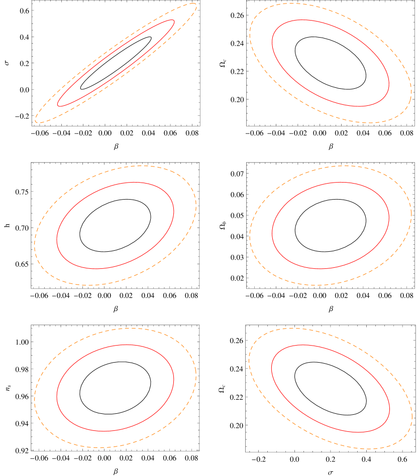
Figure A.1: Confidence ellipses for dark energy parameters in the coupled quintessence model. Shown are the ellipses for the 68%, 95% and 99% confidence level.

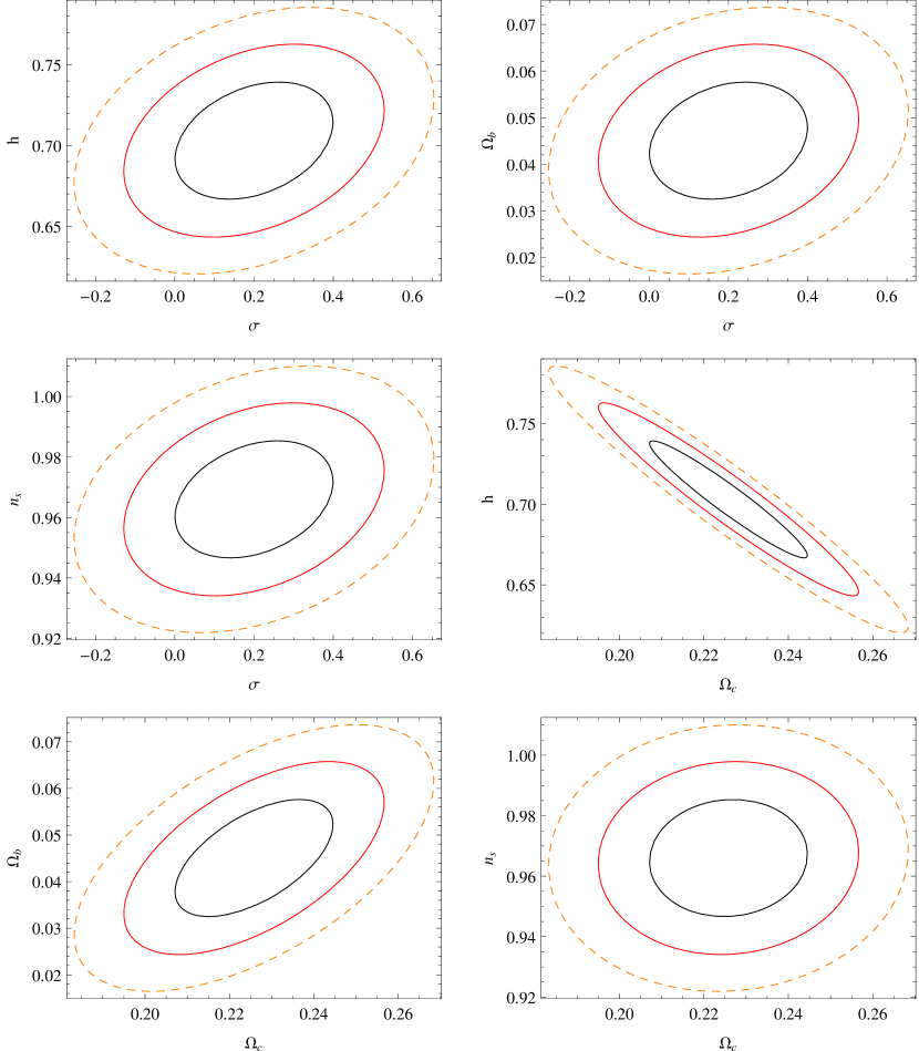
Figure A.2: Confidence ellipses for dark energy parameters in the coupled quintessence model (continued).

Erklärung

Ich versichere, dass ich diese Arbeit selbstständig verfasst habe und keine anderen als die angegebenen Quellen und Hilfsmittel benutzt habe.
Heidelberg, den 8. Juni 2011                           
(Adrian Vollmer)

References

- Albrecht et al. (2009) Albrecht, A., L. Amendola, G. Bernstein, D. Clowe, D. Eisenstein, L. Guzzo, C. Hirata, D. Huterer, R. Kirshner, E. Kolb, and R. Nichol, 2009, Findings of the Joint Dark Energy Mission Figure of Merit Science Working Group, Technical Report 2, arXiv:0901.0721.
- Albrecht et al. (2006) Albrecht, A., G. Bernstein, R. Cahn, W. L. Freedman, J. Hewitt, W. Hu, J. Huth, M. Kamionkowski, E. W. Kolb, L. Knox, J. C. Mather, S. Staggs, et al., 2006, Report of the Dark Energy Task Force, Technical Report, arXiv:astro-ph/0609591.
- Amara and Refregier (2007) Amara, A., and A. Refregier, 2007, “Systematic Bias in Cosmic Shear: Beyond the Fisher Matrix”, Monthly Notices of the Royal Astronomical Society 391(1), 11, arXiv:0710.5171v1 [astro-ph].
- Amendola (1999) Amendola, L., 1999, “Coupled Quintessence”, Physical Review D 62(4), 43511, arXiv:astro-ph/9908023.
- Amendola et al. (2006) Amendola, L., C. Charmousis, and S. C. Davis, 2006, “Constraints on Gauss-Bonnet Gravity in Dark Energy Cosmologies”, Journal of Cosmology and Astroparticle Physics 2006(12), arXiv:hep-th/0506137.
- Amendola et al. (2008) Amendola, L., M. Kunz, and D. Sapone, 2008, “Measuring the dark side (with weak lensing)”, Journal of Cosmology and Astroparticle Physics 2008(04), 013.
- Amendola and Tsujikawa (2010) Amendola, L., and S. Tsujikawa, 2010, Dark Energy: Theory and Observations (Cambridge University Press), ISBN 0521516005.
- Amendola et al. (2011) Amendola, L., P. Valeria, C. Quercellini, and A. Vollmer, 2011, “Constraining Coupled Dark Energy with Future CMB and Weak Lensing data”, to be published.
- Barausse et al. (2005) Barausse, E., S. Matarrese, and A. Riotto, 2005, “Effect of Inhomogeneities on the Luminosity Distance-Redshift Relation: Is Dark Energy Necessary in a Perturbed Universe?”, Physical Review D 71(6), 19, arXiv:astro-ph/0501152.
- Bartelmann and Schneider (1999) Bartelmann, M., and P. Schneider, 1999, “Weak Gravitational Lensing”, Physics Reports 340(4-5), 223, arXiv:astro-ph/9912508.
- Bellman (2003) Bellman, R. E., 2003, Dynamic Programming (Courier Dover Publications), ISBN 0486428095.
- Bernstein (2009) Bernstein, G. M., 2009, “Comprehensive Two-Point Analyses of Weak Gravitational Lensing Surveys”, The Astrophysical Journal 695(1), 652, arXiv:0808.3400v1 [astro-ph].
- Brumfiel (2007) Brumfiel, G., 2007, “Unseen Universe: A Constant Problem.”, Nature 448(7151), 245.
- Carroll (2003) Carroll, S., 2003, Spacetime and Geometry: An Introduction to General Relativity (Benjamin Cummings), ISBN 0805387323.
- Carroll et al. (1992) Carroll, S., W. H. Press, and E. L. Turner, 1992, “The Cosmological Constant”, Annual Review of Astronomy and Astrophysics 30(1), 499.
- Chevallier and Polarski (2001) Chevallier, M., and D. Polarski, 2001, “Accelerating Universes with Scaling Dark Matter”, International Journal of Modern Physics D 10, 213, arXiv:gr-qc/0009008.
- Copeland et al. (2006) Copeland, E. J., M. Sami, and S. Tsujikawa, 2006, “Dynamics of dark energy”, Physics , 93, arXiv:hep-th/0603057.
- De Felice and Tsujikawa (2010) De Felice, A., and S. Tsujikawa, 2010, “f(R) Theories”, Living Reviews in Relativity 13(3), 1arXiv:1002.4928v2 [gr-qc].