Theory of hadron decay into baryon-antibaryon final state

Abstract

The nonperturbative mechanism of baryon-antibaryon production due to double quark pair $(q\bar{q})$($q\bar{q})$ generation inside a hadron is considered and the amplitude is calculated as matrix element of the vertex operator between initial and final hadron wave functions. The vertex operator is expressed solely in terms of first principle input: current quark masses, string tension $\sigma$ and $\alpha_{s}$. In contrast to meson-meson production via single pair generation, in baryon case a new entity appears in the vertex: the vacuum correlation length $\lambda$, which was computed before through string tension $\sigma$. As an application electroproduction of $\Lambda_{c}\bar{\Lambda}_{c}$ was calculated and an enhancement near 4.61 GeV was found in agreement with recent experimental data.

1 Introduction

The baryon-antibaryon $(\mathcal{B}\bar{\mathcal{B}})$ final states in hadron reactions are rather typical phenomena, e.g. in charmonium decays $p\bar{p}$, $\Lambda\bar{\Lambda}$ etc. channels are significant [1]. In $e^{+}e^{-}$ collisions the ${\mathcal{B}\bar{\mathcal{B}}}$ final states are carefully studied and display in many cases $(\Lambda^{+}_{c}\Lambda^{-}_{c},\Lambda\bar{\Lambda},p\bar{p})$ a nontrivial behavior near the corresponding thresholds, see [2] for a review and references. In $B$ decays the produced $p\bar{p}$ pairs were observed with near-threshold enhancements [3]. In this paper we consider a rather general type of reactions, when a quarkonia state $(Q\bar{Q})$ decays into $\mathcal{B}\bar{\mathcal{B}}$, where $\mathcal{B}(\bar{\mathcal{B}})$ contain quark $Q$ (antiquark $\bar{Q}$). From dynamical point of view, the simplest case is the OZI allowed decay of heavy quarkonium into $\mathcal{B}\bar{\mathcal{B}}$ pair of heavy-flavor baryons, e.g. $\psi(nS)\to\Lambda^{+}_{c}\Lambda_{c}^{-}$, which was experimentally observed first in [4] at one energy, and measured in [5] in the mass interval $[4.5\div 5.4]$ GeV/$c^{2}$. For this type of reaction the creation of two light quark pairs is necessary and one could expect some suppression in this channel. However, experimentally the suppression is quite mild, as was discovered in the reaction $e^{+}e^{-}\to\Lambda^{+}_{c}\Lambda_{c}^{-}$ in [4, 5].

A peak at the $\Lambda^{+}_{c}\Lambda^{-}_{c}$ mass around 4.63 GeV/$c^{2}$ was found in [5], and the nature of this enhancement is still obscure, however different explanations were suggested [6, 7]. A discussion of possible mechanisms of similar phenomena in $\mathcal{B}\bar{\mathcal{B}}$ produced in $B$ meson decays, was given in [8]. Below we develop a systematic theory of $\mathcal{B}\bar{\mathcal{B}}$ production in OZI allowed processes, which is actually a theory of double string breaking with $\mathcal{B}\bar{\mathcal{B}}$ emission, as shown in Fig.1. As it will be seen, this theory is a one-step development of the general approach of string breaking, given in [9]. To simplify matter we consider first the case of heavy quarkonium, decaying into heavy-flavor $\mathcal{B}\bar{\mathcal{B}}$ pair.

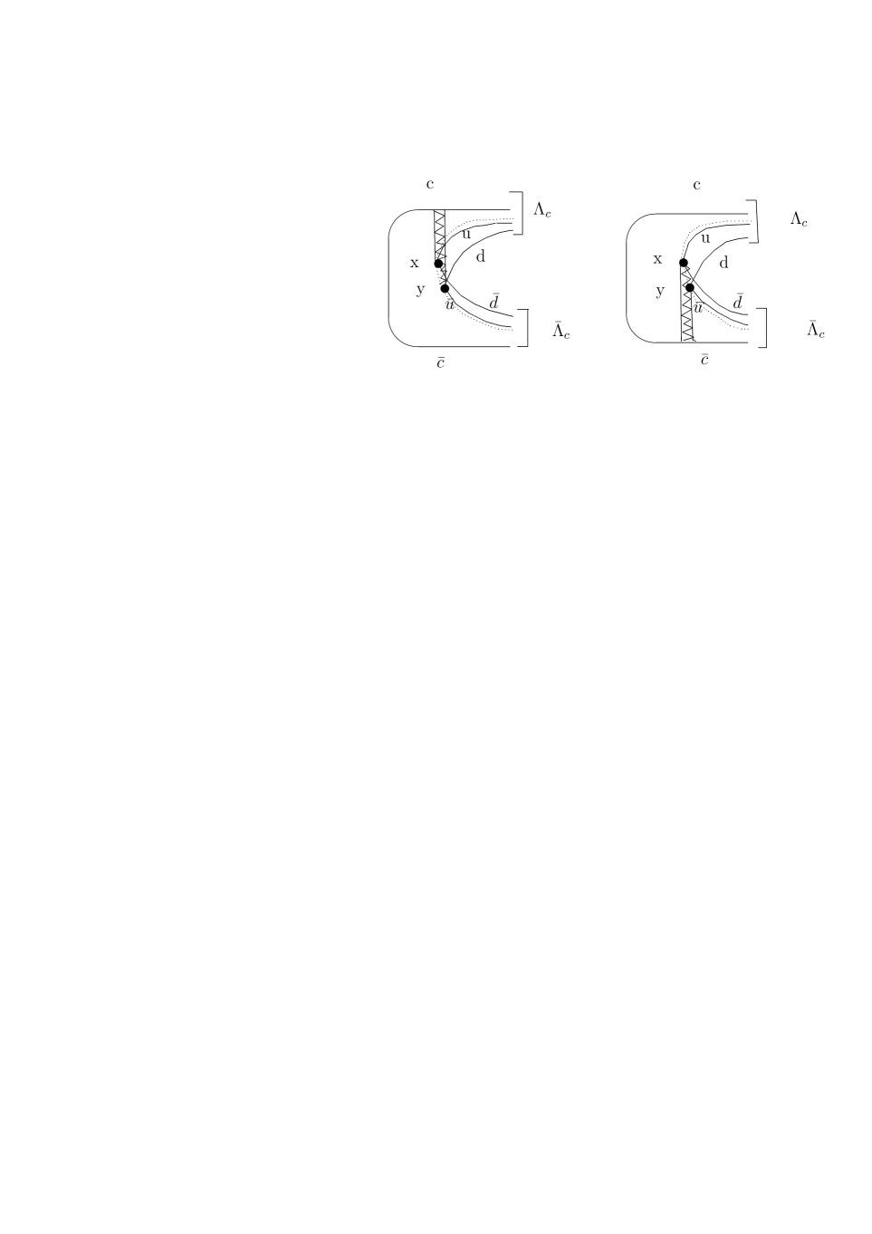
Figure 1: Double quark-pair creation at points $x,y$ in the field of heavy quarks $c\bar{c}$.

2 The formalism

The initial state of our problem is the heavy $Q\bar{Q}$ state, where $Q$ and $\bar{Q}$ are connected by a string. We are looking for a process, where two light $q\bar{q}$ pairs are created in the field of $Q\bar{Q}$, and hence the basic vertex is the $4q$ operator in the static $Q\bar{Q}$ confining field. As in the case of one pair $q\bar{q}$ vertex, it is sufficient to consider the light quark Lagrangian in the field of the static antiquark $\bar{Q}$ and static quark $Q$.

This situation is shown in Fig.1, where a pair $\bar{u}u$ is created at the point $(\mbox{\boldmath${\rm x}$},x_{4})$ and $\bar{d}d$ at $(\mbox{\boldmath${\rm y}$},y_{4})$ with time growing from left to right. The string junction trajectory is shown in Fig. 1 by dotted lines and the string junction positions at each moment of time is defined as the Torricelli points in the triangles formed by space positions of ($cud)$ and ($\bar{c}\bar{u}\bar{d})$.

It is important, that points $(\mbox{\boldmath${\rm x}$},x_{4})$ and $(\mbox{\boldmath${\rm y}$},y_{4})$ will be shown to be close to each other, and the string junction and anti-string junction are generated at one point in their vicinity, which considerably facilitates the picture of ${\mathcal{B}\bar{\mathcal{B}}}$ creation (while the latter is rather complicated in a two-step ${\mathcal{B}\bar{\mathcal{B}}}$ production).

We start with the partition function of a light quark in the field of external current of heavy quarks $Q\bar{Q}$.

$$Z=\int DAD\bar{\psi}D\psi\exp\left[-(S_{0}+S_{1}+S_{int}+S_{Q}+S_{\bar{Q}})\right],$$ (1)

$$S_{0}=\frac{1}{4}\int d^{4}x\left(F_{\mu\nu}^{a}\right)^{2},$$ (2)

$$S_{1}=-i\int d^{4}x\bar{\psi}^{f}(\hat{\partial}+m)\psi^{f},$$ (3)

$$S_{int}=-\int d^{4}x\bar{\psi}^{f}g\hat{A}^{a}t^{a}\psi^{f}.$$ (4)

Here $f$ is flavor index, $S_{Q}$ and $S_{\bar{Q}}$ refer to action of external quark currents, of (possibly high mass) quark $Q$ and antiquark $\bar{Q}$.

We exploit the background formalism [10] to split gluon field into confining background $B_{\mu}$ and perturbative gluon field $a_{\mu}$

$$A_{\mu}=B_{\mu}+a_{\mu}.$$ (5)

As in [9] we shall use the simplest contour gauge [11] to express $B_{\mu}$ in terms of field strength

$$B_{\mu}(x)=\int_{C(x)}\alpha_{\mu}(u)F_{i\mu}(u)du_{i},~{}~{}\alpha_{4}=1,~{}~{}\alpha_{i}=\frac{u_{i}}{x_{i}},$$ (6)

and the contour $C(x)$ is going from the point $x=(\mbox{\boldmath${\rm x}$},x_{4})$ to the point $(\mathbf{0},x_{4})$ on the world-line of $Q$ and then along this world-line to $x_{4}=-\infty$. Note, that our final result (11), (12) will be cast in the gauge invariant form, which is the same for all contours, connecting points $x,y$ to the world lines of $Q$ (or $\bar{Q}$). The independence of the resulting asymptotic expressions from the form of contours is shown in Appendix 3 of [13].

Averaging over fields $B_{\mu},(F_{\mu\nu})$, one can write

$$Z=\int\int D\psi D\bar{\psi}\exp\left[-(S_{1}+S_{eff})\right],$$ (7)

where $S_{eff}$ was computed in [12]-[13]. Keeping only quadratic correlators and colorelectric fields for simplicity, one obtains (for one flavor)

$$S_{eff}=-\frac{1}{2}\int d^{4}xd^{4}y\bar{\psi}(x)\gamma_{4}[\psi(x)\bar{\psi}(y)]\gamma_{4}\psi(y)J(x,y)$$ (8)

where $[\psi\bar{\psi}]$ implies color singlet combination, and $J(x,y)$ is expressed via vacuum correlator of colorelectric fields,

$$J(x,y)\equiv\frac{g^{2}}{N_{c}}\langle A_{4}(x)A_{4}(y)\rangle=\int^{x}_{0}du_{i}\int^{y}_{0}dv_{i}D(u-v).$$ (9)

Here $D(w)$ is the $np$ correlator, responsible for confinement [15],

$$\frac{g^{2}tr}{N_{c}}\langle F_{i\mu}(u)F_{k\nu}(v)\rangle=(\delta_{ik}\delta_{\mu\nu}-\delta_{i\nu}\delta_{\mu k})D(u-v)+O(D_{1})$$ (10)

and we have omitted the (vector) contribution of the correlator $D_{1}$, containing perturbative gluon exchange and nonperturbative ($np$) corrections to it.

The properties of the kernel $J(x,y)$ have been studied in [12, 13], here we only mention the general form

$$J(x,y)=\mbox{\boldmath${\rm x}$}\mbox{\boldmath${\rm y}$}f(\mbox{\boldmath${\rm x}$},\mbox{\boldmath${\rm y}$})e^{(x_{4}-y_{4})^{2}/4\lambda^{2}}D(0),$$ (11)

where we assumed the Gaussian form for simplicity $D(x)=D(0)e^{-\frac{x^{2}}{4\lambda^{2}}}$, and

$$f(\mbox{\boldmath${\rm x}$},\mbox{\boldmath${\rm y}$})=\int^{1}_{0}ds\int^{1}_{0}dte^{-(\hat{x}s-\hat{y}t)^{2}},~{}~{}\hat{x},\hat{y}=\frac{\mbox{\boldmath${\rm x}$}}{2\lambda},~{}~{}\frac{\mbox{\boldmath${\rm y}$}}{2\lambda},$$ (12)

at small $\hat{x},\hat{y}$, $f(0,0)=1$, while asymptotically

$$f(\mbox{\boldmath${\rm x}$},\mbox{\boldmath${\rm y}$})\cong\frac{\sqrt{\pi}}{\max(|\hat{x}|,|\hat{y}|)},~{}~{}\cos\theta=1,$$ (13)

where $\theta$ is the angle between ${\rm x}$ and ${\rm y}$. Note also, that $D(0)$ and $\lambda$ are connected to string tension $\sigma$

$$\sigma=2\pi\lambda^{2}D(0)=\frac{1}{2}\int D(x)d^{2}x.$$ (14)

We now turn to the effective action (8), where we write explicitly all flavor and color indices. In the latter case one should carefully restore the gauge invariant combinations, derived in [12], using parallel transporters $\Phi(u,v)=P\exp(\int^{v}_{u}A_{\mu}dz_{\mu})$ and we denote

$$\bar{\psi}_{\bar{a}}(x)\psi_{\bar{a}}(y)\equiv\bar{\psi}_{a}(x)\Phi_{ab}(x,\bar{Q},y)\psi_{b}(y)$$ (15)

with

$$\Phi_{ab}(x,\bar{Q},y)=\Phi_{ac}(\mbox{\boldmath${\rm x}$},x_{4};\mathbf{0},x_{4})\Phi_{cd}(\mathbf{0},x_{4};\mathbf{0},y_{4})\Phi_{db}(\mathbf{0},y_{4},\mbox{\boldmath${\rm y}$},y_{4}),$$ (16)

where $\mathbf{0}$ is at the position of $\bar{Q}$. Thus (8) can be rewritten as

$$S_{eff}=-\frac{1}{2}\int d^{4}xd^{4}y\bar{\psi}^{f}_{\bar{a}}(x)\gamma_{4}\psi^{f}_{\bar{b}}(x)\bar{\psi}^{g}_{\bar{b}}(y)\gamma_{4}\psi^{g}_{\bar{a}}(y)J(x,y).$$ (17)

We take now into account, that $\lambda\approx 0.1$ fm [14], [15] is much smaller, than all hadron scales, and one can integrate in (17) over $d(x_{4}-y_{4})$, using the form (11), yielding

$$S_{eff}\approx-\int d\left(\frac{x_{4}+y_{4}}{2}\right)d^{3}\mbox{\boldmath${\rm x}$}d^{3}\mbox{\boldmath${\rm y}$}(\bar{\psi}^{f}_{\bar{a}}(x)\gamma_{4}\psi^{f}_{\bar{b}}(x))(\bar{\psi}^{g}_{\bar{b}}(y)\gamma_{4}\psi^{g}_{\bar{a}}(y))\sigma(\mbox{\boldmath${\rm x}$}\mbox{\boldmath${\rm y}$})\bar{f}(\mbox{\boldmath${\rm x}$},\mbox{\boldmath${\rm y}$})$$ (18)

where we have used (14) and defined $\bar{f}(\mbox{\boldmath${\rm x}$},\mbox{\boldmath${\rm y}$})=\frac{f(\mbox{\boldmath${\rm x}$},\mbox{\boldmath${\rm y}$})}{2\lambda\sqrt{\pi}}$, so that $\bar{f}(\mbox{\boldmath${\rm x}$},\mbox{\boldmath${\rm x}$})\cong\frac{1}{|\mbox{\boldmath${\rm x}$}|}$, at large $|\mbox{\boldmath${\rm x}$}|$.

To proceed to the practical calculations with the realistic baryon wave functions, it is convenient to go over from bispinor to $2\times 2$ formalism, as it was done in [16] for $q\bar{q}$ vertices, see Appendix 2 of [16]. [Note, that the relativistic formalism for the hadron decay, developed in [9], [17], and adapted for the baryon-antibaryon case in Appendix below, accounts for the full relativistic structure of hadrons, and is exemplified in the factor $\bar{y}_{123}$, which is the ratio of the vertex $Z_{n}$ factors for all hadrons. Below we follow a much simpler derivation in terms of $2\times 2$ formalism, exploited in [16].]

We now take into account as in Appendix 2 of [16], that each bispinor $\psi$ of light quark in (18) obeys the Dirac one-body equation $(\mbox{\boldmath${\rm\alpha}$}\mbox{\boldmath${\rm p}$}+\beta(m+U))\psi=(\varepsilon-V)\psi$, where $U$ is the scalar confining interaction, $U(x)=\sigma|\mbox{\boldmath${\rm x}$}-\mbox{\boldmath${\rm x}$}_{\bar{Q}}|$, and $V$ corresponds to perturbative gluon exchanges; therefore one can write $\psi=\left(\begin{array}[]{l}v\\ w\end{array}\right)$, where

$$w=\frac{1}{m+U-V+\varepsilon}(\mbox{\boldmath${\rm\sigma}$}\mbox{\boldmath${\rm p}$})v\to\frac{1}{m+\langle U-V+\varepsilon\rangle}\mbox{\boldmath${\rm\sigma}$}\mbox{\boldmath${\rm p}$}v$$ (19)

where angular brackets imply averaged value for a given quark in the given hadron, in our case this refers to the average energy and potentials of a light quark in the produced heavy-light baryon , e.g. $\Lambda_{c}$. We also introduce for antiquarks bispinors $\psi^{c}$ and spinors $v^{c},w^{c},\psi^{c}=(v^{c},w^{c})$. Therefore

$$\bar{\psi}=C^{-1}\psi^{c}=\psi^{c}(C^{-1})^{T}=\psi^{c}\gamma_{2}\gamma_{4};\gamma_{i}=-i\beta\alpha_{i}$$

and

$$\bar{\psi}\gamma_{4}\psi=-i(v^{c},w^{c})\beta\left(\begin{array}[]{ll}0&\sigma_{2}\\ \sigma_{2}&0\end{array}\right)\left(\begin{array}[]{l}v\\ w\end{array}\right)=-i(\tilde{v}^{c},\tilde{w}^{c})\left(\begin{array}[]{l}w\\ v\end{array}\right)=-i(\tilde{v}^{c}w+\tilde{w}^{c}v)$$ (20)

where notation is used, $v^{c}\sigma_{2}\equiv\tilde{v}^{c},~{}~{}w^{c}\sigma_{2}=-\tilde{w}^{c}=-\tilde{v}^{c}\mbox{\boldmath${\rm\sigma}$}\overleftarrow{\mbox{\boldmath${\rm p}$}}\frac{1}{m+\langle U-V+\varepsilon\rangle}.$ Hence (18) can be written as (we omit below superscript $c$ in spinors $\tilde{v}^{c}$)

$$S_{eff}=\int dt_{4}d^{3}\mbox{\boldmath${\rm x}$}d^{3}\mbox{\boldmath${\rm y}$}(\tilde{v}_{\bar{a}}^{fc}(\mbox{\boldmath${\rm x}$},t_{4})Kv^{f}_{\bar{b}}(\mbox{\boldmath${\rm x}$},t_{4}))(\tilde{v}_{\bar{b}}^{g}(\mbox{\boldmath${\rm y}$},t_{4})Kv^{g}_{\bar{a}}(\mbox{\boldmath${\rm y}$},t_{4}))\sigma(\mbox{\boldmath${\rm x}$}\cdot\mbox{\boldmath${\rm y}$})\bar{f}(\mbox{\boldmath${\rm x}$},\mbox{\boldmath${\rm y}$})$$ (21)

where

$$K=\frac{1}{m+\langle U-V+\varepsilon\rangle}\mbox{\boldmath${\rm\sigma}$}\mbox{\boldmath${\rm p}$}+\mbox{\boldmath${\rm\sigma}$}\overleftarrow{\mbox{\boldmath${\rm p}$}}\frac{1}{m+\langle U-V+\varepsilon\rangle}\equiv\frac{\mbox{\boldmath${\rm\sigma}$}(\mbox{\boldmath${\rm p}$}+\overleftarrow{\mbox{\boldmath${\rm p}$}})}{\Omega}\equiv\frac{\mbox{\boldmath${\rm\sigma}$}\mbox{\boldmath${\rm P}$}}{\Omega}.$$ (22)

We now form the $S$-wave baryon wave function, which can be written as a product of a symmetric coordinate part and antisymmetric spin-flavor-color factor $A_{\mathcal{B}}$,

$$\Psi^{\mathcal{B}}=A_{\mathcal{B}}\Psi_{\mathcal{B}}^{(coord)}(\mbox{\boldmath${\rm x}$}_{1},\mbox{\boldmath${\rm x}$}_{2},\mbox{\boldmath${\rm x}$}_{3},,t_{4});~{}~{}A_{\mathcal{B}}=N_{\mathcal{B}}\sum_{ijk}\frac{1}{\sqrt{6}}e_{abc}C^{fgh}_{\alpha\beta\gamma}\varphi^{f}_{a\alpha}(i)\varphi^{g}_{b\beta}(j)\varphi^{h}_{c\gamma}(k)$$ (23)

where $abc$ are color indices, $\alpha\beta\gamma$ spinor indices and $fgh$ flavor indices.

One can separate the c.m. motion and define the set of bound state wave functions in the c.m. system $\{\psi_{h}(\mbox{\boldmath${\rm x}$}_{1}-\mbox{\boldmath${\rm x}$}_{3},\mbox{\boldmath${\rm x}$}_{2}-\mbox{\boldmath${\rm x}$}_{3})\},$

$$\Psi_{\mathcal{B}}^{(coord)}(\mbox{\boldmath${\rm x}$}_{1},\mbox{\boldmath${\rm x}$}_{2},\mbox{\boldmath${\rm x}$}_{3},,t_{4})=\frac{e^{-iEt_{4}-i\mbox{\boldmath${\rm P}$}\mbox{\boldmath${\rm R}$}}}{\sqrt{V_{3}}}\Psi_{n}(\mbox{\boldmath${\rm\xi}$},\mbox{\boldmath${\rm\eta}$}),$$ (24)

where $\mbox{\boldmath${\rm\xi}$},\mbox{\boldmath${\rm\eta}$}$ are Jacobi coordinates, which can be defined in the relativistic case as [18], $(\omega_{i}=\langle\sqrt{\mbox{\boldmath${\rm p}$}^{2}_{i}+m^{2}_{i}}\rangle,~{}~{}\omega_{+}=\sum_{i}\omega_{i})$

$$\mbox{\boldmath${\rm\eta}$}=(\mbox{\boldmath${\rm x}$}_{2}-\mbox{\boldmath${\rm x}$}_{1})\sqrt{\frac{\omega_{1}\omega_{2}}{\omega_{+}(\omega_{1}+\omega_{2})}},~{}~{}\mbox{\boldmath${\rm\xi}$}=\sqrt{\frac{\omega_{3}}{\omega_{+}^{2}(\omega_{1}+\omega_{2})}}(\omega_{1}\mbox{\boldmath${\rm x}$}_{1}+\omega_{2}\mbox{\boldmath${\rm x}$}_{2}-(\omega_{1}+\omega_{2})\mbox{\boldmath${\rm x}$}_{3})$$ (25)

and $\Psi_{n}(\mbox{\boldmath${\rm\xi}$},\mbox{\boldmath${\rm\eta}$})$ is expanded in the fast converging hyperspherical series, where the leading term ($>90\%$ in the wave function normalization, see [18], [19] for details) is a function of hyperradius only, $\Psi_{n}(\mbox{\boldmath${\rm\xi}$},\mbox{\boldmath${\rm\eta}$})\approx\psi(\rho)$, where

$$\rho^{2}=\sum^{3}_{i=1}\frac{\omega_{i}}{\omega_{+}}(\mbox{\boldmath${\rm x}$}_{i}-\mbox{\boldmath${\rm R}$})^{2}=\mbox{\boldmath${\rm\xi}$}^{2}+\mbox{\boldmath${\rm\eta}$}^{2}.$$ (26)

In what follows we shall be primarily interested in the charmed baryons, $\Lambda_{c},\sum_{c},\Xi_{c},\Omega_{c}$ and their orbital (and radial) excitations. As a first example we consider $\Lambda_{c}$ and take for simplicity only one (leading) component of wave function with singlet diquark made of $u,d$. The explicit forms of $A_{\mathcal{B}}$ for $p,\Lambda,\sum,\Xi$ are given in Appendix 1. For $\Lambda(\Lambda_{c},\Lambda_{b})$ one can write in obvious notation

$$A_{\Lambda_{c}}^{\alpha}=N_{\Lambda_{c}}\sum_{ijk}\frac{1}{\sqrt{6}}e_{abc}c_{a\alpha}(i)((ud)-(du))_{jk,bc}$$ (27)

where $(ud)_{jkbc}\equiv u_{\beta b}(j)d_{\beta c}(k)\varepsilon_{\beta}$, $\varepsilon_{\frac{1}{2}}=-\varepsilon_{-\frac{1}{2}}=1$.

As shown in Appendix 2, the gauge invariant matrix element in the c.m. system of decaying charmonium state $\Psi_{n_{1}}(\mbox{\boldmath${\rm r}$})$ can be written as

$$G(n_{1}\mbox{\boldmath${\rm P}$}_{1},n_{2}\mbox{\boldmath${\rm P}$}_{2},n_{3}\mbox{\boldmath${\rm P}$}_{3})=(2\pi)^{4}\delta^{(4)}(P_{1}-P_{2}-P_{3})J^{\mathcal{B}\mathcal{\overline{B}}}_{n_{1}n_{2}n_{3}}(\mbox{\boldmath${\rm p}$})$$ (28)

where $J^{\mathcal{B}\mathcal{\overline{B}}}_{n_{1}n_{2}n_{3}}(\mbox{\boldmath${\rm p}$})$ is

$$J^{\mathcal{B\overline{B}}}_{n_{1}n_{2}n_{3}}(\mbox{\boldmath${\rm p}$})=\int y_{123}e^{i\mbox{\boldmath${\rm p}$}\mbox{\boldmath${\rm r}$}}d^{3}(\mbox{\boldmath${\rm x}$}-\mbox{\boldmath${\rm u}$})d^{3}(\mbox{\boldmath${\rm u}$}-\mbox{\boldmath${\rm v}$})d^{3}(\mbox{\boldmath${\rm x}$}-\mbox{\boldmath${\rm y}$})(\Psi_{n_{1}}\bar{\mathcal{M}}\Psi_{n_{2}}\Psi_{n_{3}}).$$ (29)

Here $\mbox{\boldmath${\rm r}$}=c(\mbox{\boldmath${\rm u}$}-\mbox{\boldmath${\rm v}$}),~{}~{}c=\frac{\omega_{Q}}{\omega_{Q}+\omega_{u}+\omega_{d}},$ and $\Psi_{n_{i}}$ are coordinate space spinor wave functions,while $\bar{\mathcal{M}}$ is defined as

$$\bar{\mathcal{M}}=\sigma(\mbox{\boldmath${\rm x}$}\mbox{\boldmath${\rm y}$})\bar{f}(\mbox{\boldmath${\rm x}$},\mbox{\boldmath${\rm y}$})K_{x}K_{y}$$ (30)

At this point one needs to calculate the matrix element of the operator $K_{x}K_{y}$ between $\mathcal{B}\bar{\mathcal{B}}$ wavefunctions, which we write as

$$\langle A_{\bar{\mathcal{B}}}|K_{x}K_{y}(\tilde{v}_{\bar{Q}}\sigma_{i}v_{Q})|A_{\mathcal{B}}\rangle=\eta_{\mathcal{B}Q}\frac{(\mbox{\boldmath${\rm P}$}_{x}\mbox{\boldmath${\rm P}$}_{y})}{\Omega^{2}}(\tilde{v}_{\bar{\Lambda}}\sigma_{i}v_{\Lambda})$$ (31)

Explicit calculation yields coefficients $\eta_{\mathcal{B}Q}$, given in Appendix 1 for $\Lambda_{c},\sum,p,\Xi$.

It is more convenient to go over to momentum space in $J_{n_{1}n_{2}n_{3}}(\mbox{\boldmath${\rm p}$})$, and using Appendix 2, Eq. (A2.16), one has (we omit the superscript red in (A2.16) here and in what follows)

$$J^{\mathcal{B}\mathcal{\overline{B}}}_{n_{1}n_{2}n_{3}}(\mbox{\boldmath${\rm p}$})=\int\bar{y}_{123}\frac{d^{3}p_{x}}{(2\pi)^{3}}\frac{d^{3}p_{y}}{(2\pi)^{3}}\frac{d^{3}q_{x}}{(2\pi)^{3}}\frac{d^{3}q_{y}}{(2\pi)^{3}}\Psi^{+}_{n_{1}}(c\mbox{\boldmath${\rm p}$}-\mbox{\boldmath${\rm p}$}_{x}-\mbox{\boldmath${\rm p}$}_{y})\times$$

$$\times\Psi_{n_{2}}(\mbox{\boldmath${\rm p}$}_{x},\mbox{\boldmath${\rm p}$}_{y})\Psi_{n_{3}}(\mbox{\boldmath${\rm p}$}_{x}+\mbox{\boldmath${\rm q}$}_{x},\mbox{\boldmath${\rm p}$}_{y}+\mbox{\boldmath${\rm q}$}_{y})$$ (32)

where

$$\bar{y}_{123}=\frac{\mbox{\boldmath${\rm q}$}_{x}\mbox{\boldmath${\rm q}$}_{y}(\tilde{v}_{\bar{\Lambda}}\sigma_{i}v_{\Lambda})}{2\sqrt{2}N_{c}\Omega_{x}\Omega_{y}}\tilde{\mathcal{M}}(\mbox{\boldmath${\rm q}$}_{x},\mbox{\boldmath${\rm q}$}_{y})\eta_{Q\Lambda}$$ (33)

and $\tilde{\mathcal{M}}(\mbox{\boldmath${\rm q}$}_{x},\mbox{\boldmath${\rm q}$}_{y})$ is the Fourier transform of $\bar{\mathcal{M}}(\mbox{\boldmath${\rm x}$},\mbox{\boldmath${\rm y}$})$, Eq. (30), modulo $K_{x}K_{y}$, the latter were taken into account in the prefactor of $\tilde{\mathcal{M}}$ in (33). Also $\tilde{v}_{\bar{\Lambda}}$ and $v_{\Lambda}$ are spinors for $\Lambda^{-}_{c}$ and $\Lambda^{+}_{c}$ respectively, while $\sigma_{i}$ refers to the spin of $1^{--}(Q\bar{Q})_{n}$ state. From (A2.18) one can write

$$\tilde{\mathcal{M}}(\mbox{\boldmath${\rm q}$}_{x},\mbox{\boldmath${\rm q}$}_{y})=-\frac{\partial}{\partial\mbox{\boldmath${\rm q}$}_{x}}\frac{\partial}{\partial\mbox{\boldmath${\rm q}$}_{y}}\sigma\pi 4\lambda^{2}\int^{1}_{0}\int^{1}_{0}dsdt(2\pi)^{3}\delta^{(3)}(t\mbox{\boldmath${\rm q}$}_{x}+s\mbox{\boldmath${\rm q}$}_{y})e^{\frac{-\lambda^{2}(\mbox{\boldmath${\rm q}$}_{x}-\mbox{\boldmath${\rm q}$}_{y})^{2}}{(s+t)^{2}}}.$$ (34)

Insertion of (34) into (33) and (32) yields finally

$$J^{\mathcal{B}\mathcal{\overline{B}}}_{n_{1}n_{2}n_{3}}(\mbox{\boldmath${\rm p}$})=\bar{y}\int^{1}_{0}\int^{1}_{0}dsdt\int\frac{d^{3}p_{x}}{(2\pi)^{3}}\frac{d^{3}p_{y}}{(2\pi)^{3}}\frac{d^{3}Q}{(2\pi)^{3}}e^{-\lambda^{2}\mbox{\boldmath${\rm Q}$}^{2}}\Psi_{1}^{+}(c\mbox{\boldmath${\rm p}$}-\mbox{\boldmath${\rm p}$}_{x}-\mbox{\boldmath${\rm p}$}_{y})\Psi_{2}(\mbox{\boldmath${\rm p}$}_{x},\mbox{\boldmath${\rm p}$}_{y})\times$$

$$\Psi_{3}(\mbox{\boldmath${\rm p}$}_{x}+s\mbox{\boldmath${\rm Q}$},\mbox{\boldmath${\rm p}$}_{y}-t\mbox{\boldmath${\rm Q}$}),$$ (35)

where we have differentiated by parts in $(\mbox{\boldmath${\rm q}$}_{x}\mbox{\boldmath${\rm q}$}_{y})\tilde{M}(\mbox{\boldmath${\rm q}$}_{x},\mbox{\boldmath${\rm q}$}_{y})$, obtaining

$$\bar{y}=4\frac{3\cdot 2^{1/2}\pi}{N_{c}}\left(\frac{\sigma}{\Omega_{u}\Omega_{d}}\right)(\tilde{v}_{\bar{\Lambda}}\sigma_{i}v_{\Lambda})\eta_{Q\Lambda}.$$ (36)

Note the factor 4 in (36), which comes from the accounting for two diagrams in Fig.1, and two diagrams with interchanging $u$- and $d$- vertices between points ${\rm x}$ and ${\rm y}$.

3 Baryonic width of heavy quarkonium and the $\mathcal{B}\bar{\mathcal{B}}$ yield in $\mathbf{e^{+}e^{-}}$ collisions

Using $J_{n_{1}n_{2}n_{3}}(\mbox{\boldmath${\rm p}$})$ in (35), one can find the decay probability of the $n_{1}$ state of $Q\bar{Q}$ into $\mathcal{B}\bar{\mathcal{B}}$ in the states $n_{2},n_{3}$ respectively,

$$dw(1\to 23)=\overline{|J^{\mathcal{B}\mathcal{\overline{B}}}_{n_{1}n_{2}n_{3}}(\mbox{\boldmath${\rm p}$})|^{2}}(2\pi)^{4}\delta^{(4)}(\mathcal{P}_{1}-\mathcal{P}_{2}-\mathcal{P}_{3})\frac{d^{3}P_{2}d^{3}P_{3}}{(2\pi)^{6}}$$ (37)

where bar over $|J(\mbox{\boldmath${\rm p}$})|^{2}$ implies averaging over initial and sum over final spin projections; in our simple case $\overline{|\tilde{v}_{\bar{\Lambda}}\sigma_{i}v_{\Lambda}|^{2}}=1$. We now turn to a more direct experimental process of $\mathcal{B}\bar{\mathcal{B}}$ production, namely $e^{+}e^{-}\to\mathcal{B}\bar{\mathcal{B}}$, which was observed in [4, 5]. The corresponding amplitude can be written as [21]

$$A_{n_{2}n_{3}}(\mbox{\boldmath${\rm p}$},E)=\sum_{n}c_{n}(E)T_{nn_{2}n_{3}}\equiv\sum_{n,m}c_{n}(E)\left(\frac{1}{\hat{E}-E+\hat{w}(E)}\right)_{nm}J^{\mathcal{B}\mathcal{\overline{B}}}_{mn_{2}n_{3}}(\mbox{\boldmath${\rm p}$})$$ (38)

Here $\hat{E}$ and $\hat{w}$ are matrices in indices $n,m,$ of the $Q\bar{Q}$ system, $(\hat{E})_{nm}=E_{n}\delta_{nm},$

$$w_{nm}(E)=\int\frac{d^{3}p}{(2\pi)^{3}}\sum_{n_{2}n_{3}}\frac{J_{nn_{2}n_{3}}(\mbox{\boldmath${\rm p}$})J_{mn_{2}n_{3}}(\mbox{\boldmath${\rm p}$})}{E-E_{n_{2}n_{3}}(\mbox{\boldmath${\rm p}$})},$$ (39)

where $n,m$ refer to the complete set of charmonium bound states, and $J_{nn_{2}n_{3}}(\mbox{\boldmath${\rm p}$})$ is overlap integral of the $n$-th charmonium state and $n_{2},n_{3}$ states of heavy-light mesons. In terms of $A_{n_{2}n_{3}}$ the total crossection is

$$\sigma_{n_{2}n_{3}}(E)=\int|A_{n_{2}n_{3}}(\mbox{\boldmath${\rm p}$},E)|^{2}\pi\frac{d^{3}\mbox{\boldmath${\rm p}$}}{(2\pi)^{3}}\delta(E-E_{n_{2}n_{3}}(\mbox{\boldmath${\rm p}$}))$$ (40)

The factor $c_{n}(E)$ in (38) accounts for the production of $(Q\bar{Q})_{n}$ pair in the given process, in case of $e^{+}e^{-}\to(Q\bar{Q})_{n}$ one has [21]

$$c_{n}=\frac{4\pi\alpha e_{Q}\sqrt{6}}{E^{2}}\psi_{n}(0),$$

and with the definition (38)

$$\Delta R_{n_{2}n_{3}}(E)=\frac{6\pi\cdot 12e^{2}_{Q}}{E^{2}}\sum|\psi_{n}(0)T_{nn_{2}n_{3}}(E)|^{2}d\Gamma_{n_{2}n_{3}},$$ (41)

where

$$d\Gamma_{n_{2}n_{3}}=\pi\frac{d^{3}\mbox{\boldmath${\rm p}$}}{(2\pi)^{3}}\delta(E-E_{n_{2}n_{3}}(\mbox{\boldmath${\rm p}$})).$$ (42)

As a result, keeping only one state $n$ in (41) one has for

$$\Delta R_{n_{2}n_{3}}(E)=\frac{9e^{2}_{Q}p(E)\psi^{2}_{n}(0)}{E}\frac{|J^{B\bar{B}}_{n_{1}n_{2}n_{3}}(\mbox{\boldmath${\rm p}$})|^{2}}{|E_{n}-E+w_{nn}(E)|^{2}}$$ (43)

where $J^{B\bar{B}}_{n_{1}n_{2}n_{3}}(\mbox{\boldmath${\rm p}$})$ according to (A2.26) can be written as

$$J^{B\bar{B}}_{n_{1}n_{2}n_{3}}=2^{5/2}\pi^{1/4}\frac{\sigma}{\Omega^{2}}\frac{\lambda^{2}\beta_{0}^{3/2}\mathcal{R}_{n}(p)e^{-c\mbox{\boldmath${\rm p}$}^{2}R_{0}^{2}\bar{\Upsilon}}}{\left(\frac{\lambda^{2}}{R^{2}_{0}}+\bar{C}\right)^{3/2}(1+2\beta^{2}_{0}R^{2}_{0})^{3/2}},$$ (44)

where parameters $\beta_{0},R_{0},\bar{\Upsilon},\bar{C}$ refer to $(Q\bar{Q})_{n}$ and ${\mathcal{B}\mathcal{\overline{B}}}$ wave functions and are defined numerically in Appendix 2.

The polynomial $\mathcal{R}_{n}(p)$ is due to $(Q\bar{Q})_{n}$ SHO wave function, and is obtained in the way described in Eq. (A.33). It can be approximated as

$$\mathcal{R}_{n}(p)\cong-2.1\left(1-0.034\frac{p^{2}}{\beta^{2}_{0}}-0.05\left(\frac{p^{2}}{\beta^{2}_{0}}\right)^{2}\right)$$ (45)

In (44) $\bar{C}$ and $\bar{\Upsilon}$ are values of $C$ and $\Upsilon$, (A2.27),(A2.28) averaged over ($s,t$) integration region.

A rough estimate of $\Delta R^{(n)}_{\mathcal{B}\bar{\mathcal{B}}}$ in (43), using (45), near $\Lambda^{+}_{c}\Lambda_{c}^{-}$ threshold with $\psi(4S)$ state for $(Q\bar{Q})_{n}$ is

$$\Delta R^{(4)}_{\mathcal{B}\bar{\mathcal{B}}}\approx\xi\frac{p}{E}\frac{\exp(-2.5\mbox{\boldmath${\rm p}$}^{2})}{|E-E_{4}+w_{44}(E)|^{2}},$$ (46)

with

$$\xi\cong 0.9\cdot 10^{4}e^{2}_{Q}\psi^{2}_{4}(0)\left(\frac{\sigma}{\Omega^{2}}\right)^{2}\frac{\beta^{3}_{0}\lambda^{4}}{\left(\frac{\lambda^{2}}{R^{2}_{0}}+\bar{C}\right)^{3}(1+2\beta^{2}_{0}R^{2}_{0})^{3}}$$ (47)

Taking the Breit-Wigner form near the mass $E_{4}$ of $\psi(4S)$, one can write the cross section of $\sigma(e^{+}e^{-}\to\Lambda^{+}_{c}\Lambda^{-}_{c})$

$$\sigma_{4}(e^{+}e^{-}\to\Lambda_{c}^{+}\Lambda^{-}_{c})=\xi~{}2.2\cdot 10^{-4}\frac{p}{E^{3}}\frac{\exp(-2.5p^{2})}{(E-E_{4})^{2}+\frac{\Gamma^{2}_{4}}{4}}(mb),$$ (48)

where all energies are in GeV and $\sigma_{4}$ in $mb$.

To calculate $\xi$ in (47), one can use [22, 23] average energies in (A.25) with $\omega_{n}\ll\omega_{c}$, hence $a\approx 1,b\approx 0$ and average values of $s,t,\bar{s}=\bar{t}\approx 0.5$. This yields $\bar{C}\cong 0.375,\bar{\Upsilon}\cong 0.3$.

Here $E^{2}=4(\mbox{\boldmath${\rm p}$}^{2}+M^{2}_{\Lambda_{c}})$, and all momenta and energies are in GeV. One expects, that $\lambda=O(1$ GeV${}^{-1})$, as follows from the exponential fall-off of $D(x)$ in [14], this value of $\lambda$ can be varied for the Gaussian form used above. The values of $\Omega_{n}=\frac{1}{m_{n}+\langle U-V\rangle+\varepsilon_{n}},n=u,d$, where averaging is done over total baryonic state, and $m_{u},m_{d}\approx 0$, can be found from the analysis of baryons in [20], where for the light quark in a single orbital with $\sigma=0.15$ GeV² one has $\varepsilon_{u,d}\approx 380$ MeV, while $\langle U-V\rangle$ can be roughly estimated as $0.6\div 0.8$ GeV, which yields $\Omega_{n}\approx\Omega_{d}\approx(1\div 1.2)$ GeV. Now for the estimate of $\psi_{n}(0)$ one can use calculations in [22], checked $vs$ experiment, which give values of $R_{ns}(0)=\sqrt{4\pi}\psi_{ns}(0)$ with account of mixing with $(n-1)^{3}D_{1}$ states. Masses $E_{n}(~{}^{3}S_{1})$, given in Table below, are calculated in [22] (upper line) using flattening, and without flattening in [23] (lower line).

Table

n	1	2	3	4	5	6
$E_{n}$, GeV	3095	3.682	4.096	4.426	4.672	4.828
	(3.068)	(3.663)	(4.099)	(4.464)	(4.792)	(5.087)
$R_{n}(0)$, GeV3/2	0.905	0.735	0.511	0.459	0.360	$<0.445$

Inserting $R_{n}(0)=0.46$ GeV^3/2 for $n=4$, from the Table one obtains a typical value of $\xi\approx 0.035\lambda^{4}$, and the maximum of $\sigma^{(4)}$ from (48) is of the order of 1 $nb$ for $\lambda\approx 1$ GeV^-1. This magnitude is in accord with average experimental data in [5].

Note also, that $\exp(-2.5(\mbox{\boldmath${\rm p}$})^{2})$ divided by the Breit-Wigner factor in (48) is a strong cutoff factor, which decreases by a factor of 2 for $\Delta E=0.2$ GeV from the threshold. As a result, one obtains from (48) the resonance-type behavior of $\sigma^{(4)}$ with maximum around $E=4.61$ GeV, and decreasing twice at E=4.7 GeV, as shown in Fig.2. This form and the magnitude of the cross section correspond to experimental data in [6]. Explicit calculations with realistic baryon wave functions are now in progress [24].

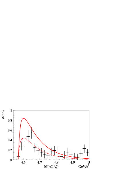
Figure 2: The cross section $\sigma(e^{+}e^{-}\to\Lambda^{+}_{c}\Lambda^{-}_{c})$ in $nb$, estimated according to Eq.(48) with $\lambda=1$ GeV^-1 as a function of total energy $E$ in GeV (solid line), experimental points are from [5], dashed line is the best normalization fit of Eq. (48) with a factor of 0.52365.

4 Summary and discussion

We have formulated above the fully nonperturbative mechanism for ${\mathcal{B}\bar{\mathcal{B}}}$ production via double quark pair generation. This mechanism is an extrapolation of the meson-meson production mechanism by string breaking, studied recently in [9]. Our main motivation is to construct a nonperturbative theory of strong decays from the first principles, in a similar way, as it was done in the theory of hadron spectra in one-channel case, where all hadron masses are computed from the first principle input: current quark masses, string tension $\sigma$ and $\alpha_{s}$, see [22, 23] for recent results and references. The simple string-breaking mechanism was indeed established with the only parameter $\sigma$ in [9], and appeared to be close to the well-known phenomenological $~{}^{3}P_{0}$ model, in this way giving a theoretical foundation for the latter. In the present case of ${\mathcal{B}\bar{\mathcal{B}}}$ production, an additional (fundamental) parameter appeared: vacuum correlation length $\lambda$, which is connected to the gluelump mass $\lambda=1/M_{gl}^{(2)}$ [14], and the latter is again expressed via string tension $\sigma$: $M^{(2)}_{gl}=6.15\sqrt{\sigma}=2.6$ GeV. In this way our first principle program is supported, however the $O(\lambda^{4})$ dependence of cross-sections makes the theory very sensitive to a possible process-depending renormalization of $\lambda$.

It is clear, that the same mechanism should work for the pair creation of other baryons, containing $c(\bar{c})$ quarks, e.g. $\Sigma_{c}\bar{\Sigma}_{c}$, $\Xi_{c}\bar{\Xi}_{c}$, the only difference will be in coefficient $\xi$ and the dominant intermediate resonance $\psi(nS)$. In the general case one should sum up over $n$, as shown in (38) and a complicated interference picture may appear.

In this case, when only $\psi(4S)$ state was kept, and this state is not far from the $\Lambda^{+}_{c}\Lambda^{-}_{c}$ threshold, the resulting bump in Fig.2 is rather prominent. In Fig. 2 the predicted theoretical enhancement is compared with experimental data from [5]. One can see a reasonable agreement.

The pair-creation mechanism, given in this paper, can be applied also to the case of light (strange) quarks $(Q\bar{Q})$. In particular, for the reaction $e^{+}e^{-}\to\Lambda\bar{\Lambda},\Sigma\bar{\Sigma}$, studied experimentally in [25], one can use the same equation (48), where the role of the intermediate state can play $\phi(2170)$ and higher $\phi$-mesons.

Since radius of high-excited $\phi$’s is much larger, than that of $\psi(4S)$, the corresponding $|\psi_{n}(0)|^{2}$ and $\beta_{0}$ in (47) are smaller, and one expects the cros sections $\sigma(e^{+}e^{-}\to\Lambda\bar{\Lambda},\Sigma\bar{\Sigma})$, to be order of magnitude smaller than those for $\Lambda_{c}\bar{\Lambda}_{c},\Sigma_{c}\bar{\Sigma}_{c}$. This is supported by experiments in [25].

As for the case of the cross section $\sigma(e^{+}e^{-}\to\Lambda_{b}\bar{\Lambda}_{b},\Sigma_{b}\bar{\Sigma}_{b})$, our Eq. (48) applies here without modifications, except for the replacement of $\psi(4S)$ by $\Upsilon(6S)$; the main suppression factor comes from $E^{3}$ in the denominator of (48) and from $\left(\frac{e_{b}}{e_{c}}\right)^{2}=\frac{1}{4}$, while $|\psi_{n}(0)|^{2}$ acquires factor 8.6, since $R_{6}(0)=1.35$ GeV^3/2 [26]. As a result the cross section for $\Lambda_{b}\bar{\Lambda}_{b}$ production is one order of magnitude smaller than that for $\Lambda_{c}\bar{\Lambda}_{c}$ production.

One should stress, that the theory, developed here and in [9], can be applied to string-breaking processes, where the energy transfer $\Delta E$ from “external” quarks $Q\bar{Q}$ to the pair-production vertex is not large, $\Delta E\cdot\lambda\mathrel{\mathchoice{\lower 3.6pt\vbox{\halign{$\mathsurround=0pt\displaystyle\hfil#\hfil$\cr<\crcr\sim\crcr}}}{\lower 3.6pt\vbox{\halign{$\mathsurround=0pt\textstyle\hfil#\hfil$\cr<\crcr\sim\crcr}}}{\lower 3.6pt\vbox{\halign{$\mathsurround=0pt\scriptstyle\hfil#\hfil$\cr<\crcr\sim\crcr}}}{\lower 3.6pt\vbox{\halign{$\mathsurround=0pt\scriptscriptstyle\hfil#\hfil$\cr<\crcr\sim\crcr}}}}1$. In the opposite case one should take $\Delta E$ into account in the string profile function $J(x,y)$ in (11), which strongly changes result, these effects are now under investigation.

The theory, proposed above, is purely nonperturbative and therefore quite different from the mostly perturbative approach, developed before for ${\mathcal{B}\bar{\mathcal{B}}}$ production (see [8], [27] for discussion and references). In this respect two approaches complement each other and the final goal can be to formulate the unified theory, where all particle yields are expressed via first principle constants.

The author is grateful to A.M.Badalian, I.M.Narodetski, and M.A.Trusov for discussions and comments. Useful advices, suggestions and help of G.V.Pakhlova in preparing Fig.2 of the present paper are gratefully acknowledged.The financial support of the Grant RFBR No 09-02-00620a is acknowledged.

Appendix 1

Baryon total wave function in terms of individual quark spinors

$$A_{\mathcal{B}}=N_{\mathcal{B}}\sum_{abc}\frac{e_{abc}}{\sqrt{6}}\sum_{ijk}C^{\mathcal{B}}(fgh|\alpha\beta\gamma)v^{f}_{\alpha}(a,i)v^{g}_{\beta}(b,j)v^{h}_{\gamma}(c,k).$$ (A1.1)

We use notations $v^{u}_{\frac{1}{2}}(a,i)\equiv u_{+}(a,i),~{}~{}v^{d}_{\frac{1}{2}}(b,j)=d_{+}(b,j)$, etc. Here $i,j,k=1,2,3$ and $\sum_{ijk}$ denotes permutations of 1,2,3, we also require $j<k$, then the proton wave function with spin up can be written as (color indices are suppressed for simplicity).

$$A_{{p}}=N_{p}\sum_{abc}\frac{e_{abc}}{\sqrt{6}}\sum_{ijk}u_{+}(i)[(d(j)u(k))-(u(j)d(k))].$$ (A1.2)

Here notation is used: $(du)=d_{-}u_{+}-d_{+}u_{-};~{}~{}N_{p}=\frac{1}{3\sqrt{2}}$.

For $\Lambda(J=\frac{1}{2})$ hyperon with spin up one can write

$$A_{{\Lambda}}=N_{\Lambda}\sum_{abc}\frac{e_{abc}}{\sqrt{6}}\sum_{ijk}s_{+}(i)[(u(j)d(k))-(d(j)u(k))],$$ (A1.3)

and $N_{\Lambda}=\frac{1}{\sqrt{12}}$.

For $\Sigma$ hyperons with spin up

$$A_{\Sigma^{0}}=N_{\Sigma^{0}}\sum_{ijk}\sum_{abc}\frac{e_{abc}}{\sqrt{6}}\{s_{+}(i)([ud]_{0}+[du]_{0})-2s_{-}(i)[ud]_{++}\},$$ (A1.4)

where $N_{\Sigma^{0}}=\frac{1}{6}$ and $[ud]_{0}=u_{+}(j)d_{-}(k)+u_{-}(j)d_{+}(k),$

$$[ud]_{++}=u_{+}(j)d_{+}(k)+d_{+}(j)u_{+}(k).$$

$$A_{\Sigma^{+}}=N_{\Sigma^{+}}\sum_{ijk}\sum_{abc}\frac{e_{abc}}{\sqrt{6}}\{s_{+}(i)([udu]_{0}-2s_{-}(i)u_{+}(j)u_{+}(k)\},$$ (A1.5)

where $N_{\Sigma^{+}}=\sqrt{2}/6$. For ${\Sigma^{-}}$ one replaces in (A1.5) all $u$ quarks by $d$ quarks. For $\Xi^{0}$ hyperon one has

$$A_{\Xi^{0}}=A_{\Sigma^{+}}(u\leftrightarrow s).$$

As a result of calculations of $\eta_{Q\mathcal{B}}$ one obtains

$$\eta_{s\Lambda}=1,~{}~{}\eta_{s\Sigma}=\frac{1}{9}=\eta_{u\Xi^{0}};~{}~{}\eta_{up}=\frac{4}{3},~{}~{}\eta_{u\Lambda}=\frac{1}{3\sqrt{2}}.$$ (A1.6)

In the last two coefficients one must take into account the contribution of $u$ quark in the vector meson $(u\bar{u})_{n}$, which gets into the singlet pair $(ud)$ or $(du)$. This contribution is proportional to $\tilde{v}_{\bar{\mathcal{B}}}\mbox{\boldmath${\rm\sigma}$}\mbox{\boldmath${\rm P}$}v\cdot P_{i}\to\frac{1}{3}\tilde{v}_{\bar{\mathcal{B}}}\sigma_{i}v_{\bar{\mathcal{B}}}\mbox{\boldmath${\rm P}$}^{2}$. In case of $\eta_{u\Lambda}$ the isosinglet component of $(u\bar{u})_{n}$ gives an extra factor of $\frac{1}{\sqrt{2}}$.

Appendix 2

Relativistic derivation of the hadron $\to\mathcal{B\overline{B}}$ amplitude

We start with the fully relativistic formalism and we follow here the derivation given in [17]. The initial stage is the point-to-point amplitude, which is the Green’s function $G_{123xy}$ for $c\bar{c}$ state emitted at point 1 and baryons absorbed at points 2 and 3, while intermediate points $x,y$ are the same as in the main text, i.e. where two light quark pairs of flavors $f$ and $g$ respectively are emitted, see Fig.1.

One can write this amplitude as

$$\int G_{123xy}d^{4}xd^{4}y=\int d^{4}xd^{4}ytr(\Gamma_{1}S_{Q}(1,2)\Gamma_{2}S^{f}_{q}(2,x)S^{g}_{q}(2,y)\times$$

$$\times\Gamma_{x}\mathcal{M}(x,y)\Gamma_{y}S^{f}_{q}(x,3)S_{q}^{g}(y,3)\Gamma_{3}S_{q}(3,1))\equiv\langle 0|j_{Q}(1)j_{\mathcal{B}}(2)\mathcal{M}j_{\bar{\mathcal{B}}}(3)|0\rangle$$ (A2.1)

where $S_{q,Q}$ are light $(q)$ and heavy $(Q)$ quark propagators, and $\Gamma_{i}$ are vertices for given hadrons, e.g. $\Gamma_{1}=\gamma_{i}$ for $1^{--}$ state of charmonia etc., while $\Gamma_{x}=\Gamma_{y}=\gamma_{4}$. Finally,

$$\mathcal{M}(x,y)=\sigma(\mbox{\boldmath${\rm x}$}\mbox{\boldmath${\rm y}$})\bar{f}(\mbox{\boldmath${\rm x}$},\mbox{\boldmath${\rm y}$})$$ (A2.2)

and one should integrate (A2.1) over $d^{4}xd^{4}y$. However, the physical amplitude of a hadron decay into two hadrons $A(n_{1}\mbox{\boldmath${\rm P}$}_{1};n_{2}\mbox{\boldmath${\rm P}$}_{2},n_{3}\mbox{\boldmath${\rm P}$}_{3})$ should be obtained from $G_{123xy}$ in two steps: 1) first one should go from coordinate points 1,2,3 to definite momentum states $\mbox{\boldmath${\rm P}$}_{1},\mbox{\boldmath${\rm P}$}_{2},\mbox{\boldmath${\rm P}$}_{3}$, and 2) one should go from point-to-point amplitude to hadron-to hadron amplitude, which is obtained by amputating in the matrix element (A2.1) the pieces $\langle 0|j_{i}|n_{i}\mbox{\boldmath${\rm P}$}_{i}\rangle$, which are proportional to hadron decay constant. E.g. for a vector meson

$$\langle 0|j^{\Gamma}_{k}|n,\mbox{\boldmath${\rm P}$}=0\rangle=\varepsilon_{k}\sqrt{\frac{M_{n}}{2}}f^{(n)}_{\Gamma}$$ (A2.3)

Proceeding as in Appendix 2 of [17], one arrives at the expression

$$A(n_{1}\mbox{\boldmath${\rm P}$}_{1};n_{2}\mbox{\boldmath${\rm P}$}_{2},n_{3}\mbox{\boldmath${\rm p}$}_{3})=(2\pi)^{4}\delta^{(4)}(\mathcal{P}_{1}-\mathcal{P}_{2}-\mathcal{P}_{3})J_{n_{1}n_{2}n_{3}}^{(rel)}(\mbox{\boldmath${\rm p}$})$$ (A2.4)

where

$$J^{rel}_{n_{1}n_{2}n_{3}}(\mbox{\boldmath${\rm p}$})=\frac{1}{N_{c}}\int\bar{y}_{123}d^{3}(x-u)d^{3}(u-v)d^{3}(x-y)\Psi_{n_{1}}(\mbox{\boldmath${\rm u}$}-\mbox{\boldmath${\rm v}$})\sigma(\mbox{\boldmath${\rm x}$}\mbox{\boldmath${\rm y}$})e^{i\mbox{\boldmath${\rm p}$}\mbox{\boldmath${\rm r}$}}\bar{f}(\mbox{\boldmath${\rm x}$}\mbox{\boldmath${\rm y}$})\times$$

$$\times\Psi_{n_{2}}(\mbox{\boldmath${\rm x}$}-\mbox{\boldmath${\rm u}$},\mbox{\boldmath${\rm y}$}-\mbox{\boldmath${\rm u}$})\Psi_{n_{3}}(\mbox{\boldmath${\rm x}$}-\mbox{\boldmath${\rm v}$},\mbox{\boldmath${\rm y}$}-\mbox{\boldmath${\rm v}$}),$$ (A2.5)

and $\mbox{\boldmath${\rm r}$}=c(\mbox{\boldmath${\rm u}$}-\mbox{\boldmath${\rm v}$}),~{}~{}c=\frac{\omega_{c}}{\omega_{c}+\omega_{u}+\omega_{d}}$, where $\omega_{i}$ is average kinetic energy of quark $i$ in the hadron. Here $\Psi_{n_{i}}$ are coordinate parts of wave functions, and $\bar{y}_{123}$ is computed as a ratio of total trace and hadron $Z_{i}$ factors, (see Appendix 2 of [17] for details)

$$\bar{y}_{123}=\frac{Z_{123xy}}{\sqrt{Z_{1}Z_{2}Z_{3}}},~{}~{}Z_{1}=tr(\Gamma_{1}\Lambda_{Q}\Gamma_{1}\Lambda_{\bar{Q}})$$ (A2.6)

$$Z_{k}(k=2,3)=tr(\Gamma_{k}\prod^{3}_{s=1}\frac{(m-i\hat{p}_{s})}{2\omega_{s}}\Gamma_{k})$$ (A2.7)

$$Z_{123xy}=tr(\Gamma_{i}\Lambda_{Q}\Gamma_{2}(\Lambda_{\bar{q}}\gamma_{4}\Lambda_{q})(\Lambda_{\bar{q}}\gamma_{4}\Lambda_{q})\Gamma_{3}\Lambda_{\bar{Q}})$$ (A2.8)

and

$$\Lambda_{q}=\frac{m_{q}-ip\gamma_{i}+\omega_{q}\gamma_{4}}{2\omega_{q}},~{}~{}\Lambda_{\bar{q}}=\frac{m_{\bar{q}}-ip\gamma_{i}-\omega_{q}\gamma_{4}}{2\omega_{q}}.$$ (A2.9)

Here $\omega_{q}=\langle\sqrt{m^{2}_{q}+\mbox{\boldmath${\rm p}$}^{2}}\rangle$, where the average is for the given hadron $n$.

Examples of $\bar{y}_{123}$ for meson$\to$ 2 meson decay are given in [16, 17].

A much simpler derivation can be made in the so-called Dirac formalism, introduced in [16]. In this case the final expressions are given in the form of $2\times 2$ matrices and it is convenient in this case to write in (A2.4) the Dirac-reduced expression $J^{red}_{n_{1}n_{2}n_{3}}$ instead of $J^{rel}_{n_{1}n_{2}n_{3}}$, and the former is best written in the momentum space (first in the simpler case, when $\mathcal{M}(x,y)$ in (A2.2) is taken as an effective constant $\bar{\mathcal{M}}$).

$$J^{{}^{\prime}red}_{n_{1}n_{2}n_{3}}(\mbox{\boldmath${\rm p}$})=\int y^{\prime}_{red}\frac{d^{3}p_{x}}{(2\pi)^{3}}\frac{d^{3}p_{y}}{(2\pi)^{3}}\Psi^{+}_{n_{1}}(c\mathbf{p}-\mathbf{p}_{x}-\mathbf{p}_{y})\Psi_{n_{2}}(\mathbf{p}_{x},\mathbf{p}_{y})\Psi_{n_{3}}(-\mathbf{p}_{x},-\mathbf{p}_{y})$$ (A2.10)

where

$$y^{\prime}_{red}=tr\{\Gamma^{(n_{1})}_{red}\Gamma_{red}^{(n_{2})}K(p_{x})\bar{\mathcal{M}}K(p_{y})\Gamma^{(n_{3})}_{red}\},$$ (A2.11)

and $K$ defined in (22).

Note, that (A2.11) has the same structure, as Eq. (B3) in [16], with ($\mbox{\boldmath${\rm\sigma}$}\mbox{\boldmath${\rm q}$})$ replaced by $K\mathbf{M}K$ in (A2.11).

As follows from the Table VII in [16], the reduced vertex $\Gamma_{red}^{(n_{1})}=\frac{1}{\sqrt{2}}\sigma_{i}$ for $~{}^{3}S_{1}$ state $(1^{--}$) of charmonium, while for $\Gamma_{red}^{(n_{k})},k=2,3$, one must choose the appropriate baryon vertex, which is given in Appendix 1. To illustrate our procedure, we consider a simplified example (where color indices are suppressed, but the final result coincides with the exact one) of a baryon, consisting of singlet $(ud)$ pair plus $c$ quark, as

$$(\Gamma^{(n_{2})}_{red})_{\alpha\beta\gamma}=\frac{\varepsilon_{\alpha\beta}}{\sqrt{2}}\chi_{\gamma};(\Gamma^{(n_{3})}_{red})_{\alpha^{\prime}\beta^{\prime}\gamma^{\prime}}=\frac{\varepsilon_{\alpha^{\prime}\beta^{\prime}}}{\sqrt{2}}\chi_{\gamma^{\prime}}^{+}.$$ (A2.12)

Now, introducing ${\rm P}$ in $K(\mbox{\boldmath${\rm P}$})$, so that $K=\frac{\mbox{\boldmath${\rm\sigma}$}\mbox{\boldmath${\rm P}$}}{\Omega}$, with $\mbox{\boldmath${\rm P}$}=\mbox{\boldmath${\rm p}$}+\overleftarrow{\mbox{\boldmath${\rm p}$}}$,

$$\varepsilon K(\mbox{\boldmath${\rm P}$}_{x})K(\mbox{\boldmath${\rm P}$}_{y})\varepsilon=\varepsilon_{\beta\gamma}K_{\beta\alpha}(\mbox{\boldmath${\rm P}$}_{x})K_{\gamma\delta}(\mbox{\boldmath${\rm P}$}_{y})\varepsilon_{\alpha\delta},$$

one obtains

$$(\varepsilon KK\varepsilon)=-\frac{2\mbox{\boldmath${\rm P}$}_{x}\mbox{\boldmath${\rm P}$}_{y}}{\Omega_{x}\Omega_{y}}$$ (A2.13)

and finally

$$y^{red}=-\frac{1}{\sqrt{2}}\frac{\mbox{\boldmath${\rm P}$}_{x}\mbox{\boldmath${\rm P}$}_{y}}{\Omega_{x}\Omega_{y}}(\chi^{+}\mbox{\boldmath${\rm\sigma}$}_{i}\chi)\bar{\mathcal{M}}$$ (A2.14)

and for $\Omega_{x}\Omega_{y}$ can be assigned the values $\Omega_{u},\Omega_{d}$ (or vice versa) with $\Omega_{u,d}={m_{u,d}+\langle U-V\rangle+\varepsilon_{u,d}}$.

However, $\Omega_{u,d}$ in (A2.13) can be easily extracted from $K$ in Eq. (22) of the main text, and one can see, that in the approximation, when the denominator in $K$ is kept constant (independent of ${\rm x}$ or ${\rm y}$) $K_{x}\sim\mbox{\boldmath${\rm\sigma}$}(\mbox{\boldmath${\rm p}$}_{x}+\mbox{\boldmath${\rm p}$}^{\prime}_{x})=0$. Therefore one must now take into account the coordinate dependence of $\mathcal{M}(x,y)$ in (A2.2) and we write

$$\mathcal{M}(x,y)=\mathcal{M}(\mbox{\boldmath${\rm x}$}-\mbox{\boldmath${\rm u}$},\mbox{\boldmath${\rm y}$}-\mbox{\boldmath${\rm u}$})=\int\tilde{\mathcal{M}}(\mbox{\boldmath${\rm q}$}_{x},\mbox{\boldmath${\rm q}$}_{y})\frac{d^{3}q_{x}}{(2\pi)^{3}}\frac{d^{3}q_{x}}{(2\pi)^{3}}e^{i\mbox{\boldmath${\rm q}$}_{x}(\mbox{\boldmath${\rm x}$}-\mbox{\boldmath${\rm u}$})+i\mbox{\boldmath${\rm q}$}_{y}(\mbox{\boldmath${\rm y}$}-\mbox{\boldmath${\rm u}$})}$$ (A2.15)

and (A2.10), (A2.11) are replaced by

$$J^{red}_{n_{1}n_{2}n_{3}}(\mbox{\boldmath${\rm p}$})=\int\bar{y}^{red}\frac{d^{3}p_{x}}{(2\pi)^{3}}\frac{d^{3}p_{y}}{(2\pi)^{3}}\frac{d^{3}q_{x}}{(2\pi)^{3}}\frac{d^{3}q_{y}}{(2\pi)^{3}}\Psi^{+}_{n_{1}}(p-p_{x}-p_{y})\times$$ (A2.16)

$$\times\Psi_{n_{2}}(p_{x},p_{y})\Psi_{n_{3}}(-p_{x}-q_{x},-p_{y}-q_{y})$$

where $y^{{}^{\prime}red}$ in (A2.10) is replaced by $\bar{y}^{red}=y^{red}\tilde{\mathcal{M}}(q_{x},q_{y})$, and $y^{red}$ in (A2.14)

Here $\mathcal{M}(q_{x},q_{y})$ is the Fourier transform of $\mathcal{M}(x,y)$ (A2.2),

$$\mathcal{M}(q_{x},q_{y})=\int\int d^{3}xd^{3}y\frac{\sigma(\mbox{\boldmath${\rm x}$}\mbox{\boldmath${\rm y}$})}{2\lambda\sqrt{\pi}}\int^{1}_{0}\int^{1}_{0}dsdt\exp\left[-\frac{(\mbox{\boldmath${\rm x}$}s-\mbox{\boldmath${\rm y}$}t)^{2}}{4\lambda^{2}}\right]e^{-i\mbox{\boldmath${\rm q}$}_{x}\mbox{\boldmath${\rm x}$}-i\mbox{\boldmath${\rm q}$}_{y}\mbox{\boldmath${\rm y}$}}.$$ (A2.17)

Performing the integrals, one obtains

$$\mathcal{M}(\mbox{\boldmath${\rm q}$}_{x},\mbox{\boldmath${\rm q}$}_{y})=-\frac{\partial}{\partial\mbox{\boldmath${\rm q}$}_{x}}\frac{\partial}{\partial\mbox{\boldmath${\rm q}$}_{y}}\frac{\sigma\pi^{3/2}}{2\lambda\sqrt{\pi}}(2\lambda)^{3}\int^{1}_{0}\int^{1}_{0}dsdt(2\pi)^{3}\delta^{(3)}(t\mbox{\boldmath${\rm q}$}_{x}+s\mbox{\boldmath${\rm q}$}_{y})e^{-\frac{\lambda^{2}(\mbox{\boldmath${\rm q}$}_{x}-\mbox{\boldmath${\rm q}$}_{y})^{2}}{(s+t)^{3}}}.$$ (A2.18)

Insertion of (A2.18) into (A2.16) yields (after integrating out $\delta$- function in (A2.18) and differentiating $\frac{\partial}{\partial\mbox{\boldmath${\rm q}$}_{x}}~{}~{}\frac{\partial}{\partial\mbox{\boldmath${\rm q}$}_{y}}$ by parts)

$$J^{red}_{n_{1}n_{2}n_{3}}(\mbox{\boldmath${\rm p}$})\equiv J(\mbox{\boldmath${\rm p}$})=\int^{1}_{0}\int^{1}_{0}dsdt~{}~{}\bar{y}^{\rm red}\int\frac{d^{3}p_{x}}{(2\pi)^{3}}\frac{d^{3}p_{y}}{(2\pi)^{3}}\frac{d^{3}Q}{(2\pi)^{3}}\Psi_{1}(c\mbox{\boldmath${\rm p}$}-\mbox{\boldmath${\rm p}$}_{x}-\mbox{\boldmath${\rm p}$}_{y})\times$$ (A2.19)

$$\Psi_{2}(\mbox{\boldmath${\rm p}$}_{x},\mbox{\boldmath${\rm p}$}_{y})\Psi_{3}(\mbox{\boldmath${\rm p}$}_{x}+s\mbox{\boldmath${\rm Q}$};\mbox{\boldmath${\rm p}$}_{y}-t\mbox{\boldmath${\rm Q}$}),$$

where $\bar{y}^{\rm red}$ is now

$$\bar{y}^{\rm red}=\frac{3\cdot 2^{1/2}\lambda^{2}\pi\sigma(\chi^{+}\sigma_{i}\chi)}{N_{c}\Omega_{u}\Omega_{d}}e^{-\lambda^{2}\mbox{\boldmath${\rm Q}$}^{2}}.$$ (A2.20)

To estimate the integral in (A2.19) we use the oscillator wave functions for $\Psi_{1}$, and oscillator form of hyperspherical wave function for $\Psi_{2},\Psi_{3}$,

$$\Psi_{1}(\mbox{\boldmath${\rm x}$})=\mathcal{P}(\mbox{\boldmath${\rm x}$})\exp\left(-\frac{\beta^{2}_{0}x^{2}}{2}\right),~{}~{}\Psi_{2}(\rho)=N\exp\left(-\frac{\rho^{2}}{\rho^{2}_{0}}\right),$$ (A2.21)

where $\rho^{2}=\mbox{\boldmath${\rm\xi}$}^{2}+\mbox{\boldmath${\rm\eta}$}^{2}=\sum^{3}_{i=1}(\mbox{\boldmath${\rm x}$}^{(i)}-\mbox{\boldmath${\rm R}$})^{2}\frac{\omega_{i}}{\omega_{+}},~{}~{}\omega_{i}=\langle\sqrt{p^{2}_{i}+m^{2}_{i}}\rangle,~{}~{}\omega_{+}=\sum^{3}_{i=1}\omega_{i}$ $\omega_{u}\cong\omega_{d}\equiv\omega_{n}.$

In $p$-space one can use (see (25) and [18] for relations between standard and Jacobi coordinates)

$$\Psi_{2}=N_{2}\exp(-R^{2}_{0}(\mbox{\boldmath${\rm p}$}^{2}_{\xi}+\mbox{\boldmath${\rm p}$}^{2}_{\eta})),~{}~{}N^{2}_{2}=(8\pi R^{2}_{0})^{3}$$ (A2.22)

and $\mbox{\boldmath${\rm p}$}_{\xi}=\sqrt{\frac{\omega_{+}}{2\omega_{c}}}(\mbox{\boldmath${\rm p}$}_{x}+\mbox{\boldmath${\rm p}$}_{y}),~{}~{}\mbox{\boldmath${\rm p}$}_{\eta}=\frac{1}{\sqrt{2}}(\mbox{\boldmath${\rm p}$}_{y}-\mbox{\boldmath${\rm p}$}_{x})$.

Relation between average $\langle\rho^{2}\rangle$ and $R^{2}_{0}$ is $\langle\rho^{2}\rangle=6R^{2}_{0}=\langle r^{2}_{\mathcal{B}}\rangle$. For $\Psi_{1}$ one can first take for simplicity $\Psi_{1}(p)=N_{1}\exp\left(-\frac{\mbox{\boldmath${\rm p}$}^{2}}{2\beta^{2}_{0}}\right).$

Now one can integrate in(A2.19) over $d^{3}p_{x}d^{3}p_{y}$, which yields

$$I(\mbox{\boldmath${\rm p}$},\mbox{\boldmath${\rm Q}$})\equiv\int\frac{d^{3}p_{x}}{(2\pi)^{3}}\frac{d^{3}p_{y}}{(2\pi)^{3}}\Psi_{1}(c\mbox{\boldmath${\rm p}$}-\mbox{\boldmath${\rm p}$}_{x}-\mbox{\boldmath${\rm p}$}_{y})\Psi_{2}(\mbox{\boldmath${\rm p}$}_{x},\mbox{\boldmath${\rm p}$}_{y})\Psi_{3}(\mbox{\boldmath${\rm p}$}_{x}+s\mbox{\boldmath${\rm Q}$},\mbox{\boldmath${\rm p}$}_{y}-t\mbox{\boldmath${\rm Q}$})=$$

$$=N_{1}N_{2}^{2}\left(\frac{1}{\sqrt{d_{1}(a-b)R^{2}_{0}}8\pi}\right)^{3}\exp(-\Xi),$$ (A2.23)

where

$$\Xi=\frac{(c\mbox{\boldmath${\rm p}$})^{2}}{2\beta^{2}_{0}}+aR^{2}_{0}\mbox{\boldmath${\rm Q}$}^{2}(s^{2}+t^{2})-2bR^{2}_{0}\mbox{\boldmath${\rm Q}$}^{2}st-\frac{\mathbf{d}^{2}_{2}}{4d_{1}}-\frac{(s+t)^{2}}{4}\mbox{\boldmath${\rm Q}$}^{2}R^{2}_{0}(a-b)$$ (A2.24)

and

$$a=\frac{(\omega_{+}+\omega_{c})}{2\omega_{c}},~{}~{}b=\frac{\omega_{n}}{\omega_{c}},~{}~{}d_{1}=\frac{1}{2\beta^{2}_{0}}+R^{2}_{0}(a+b);~{}~{}\mathbf{d}_{2}=-\frac{c\mbox{\boldmath${\rm p}$}}{\beta^{2}_{0}}+R^{2}_{0}(a+b)\mbox{\boldmath${\rm Q}$}(s-t).$$ (A2.25)

Finally the integration over $d^{3}Q$ can be done in (A2.19), yielding

$$J(\mbox{\boldmath${\rm p}$})=\tilde{y}^{\rm red}\frac{N_{1}N_{2}^{2}}{(4\pi)^{6}}\int^{1}_{0}\int^{1}_{0}dsdt\left[\frac{\pi}{(\lambda^{2}+CR^{2}_{0})d_{1}R_{0}^{2}(a-b)}\right]^{3/2}\exp[-R^{2}_{0}(c\mbox{\boldmath${\rm p}$})^{2}\Upsilon]$$ (A2.26)

where

$$\Upsilon=\frac{a+b}{1+2\beta^{2}_{0}R^{2}_{0}(a+b)}-\left(\frac{a+b}{1+2\beta^{2}_{0}R^{2}_{0}(a+b)}\right)^{2}\frac{R^{2}_{0}}{4(\lambda^{2}+CR^{2}_{0})},$$ (A2.27)

and

$$C=a(s^{2}+t^{2})-2bst-\frac{(s+t)^{2}}{4}(a-b)-\frac{(a+b)^{2}(s-t)^{2}R^{2}_{0}\beta^{2}_{0}}{2(1+2\beta^{2}_{0}R^{2}_{0}(a+b))},$$ (A2.28)

$$\tilde{y}^{red}=\frac{3\cdot 2^{3/2}\pi\lambda^{2}\sigma(\chi^{+}\sigma_{i}\chi)}{N_{c}\Omega_{u}\Omega_{d}}$$ (A2.29)

In (A2.26) $N_{1}=\left(\frac{8\pi}{2\beta^{2}_{0}}\right)^{3/4}$, if the SHO for $\psi_{1}$ is used.

For $(n^{3}S_{1})c\bar{c}$ state in the same oscillator basis one should use instead, as in [16]

$$\Psi_{1}(n^{3}S_{1})=\frac{1}{\sqrt{4\pi}}R^{SHO}_{n}(\beta_{0},p)=\frac{(-)^{n}(2\pi)^{3/2}}{\sqrt{4\pi}\beta_{0}^{3/2}}\sqrt{\frac{2(n-1)!}{\Gamma(n+\frac{1}{2})}}e^{-\frac{p^{2}}{2\beta^{2}_{0}}}L^{1/2}_{n-1}\left(\frac{p^{2}}{\beta^{2}_{0}}\right)$$ (A2.30)

normalized as $\int|\Psi_{1}|^{2}\frac{d^{3}p}{(2\pi)^{3}}=1$.

To understand the structure of the obtained result (A2.25), one can use the limit of large mass $m_{Q}$, i.e. $\omega_{c}\gg\omega_{n}$, $n=u,d$, which yields $a=1,b=0$. Another useful limit is a) $2\beta^{2}_{0}R^{2}_{0}\gg 1$, which is achieved for large size baryons as compared to the radius of charmonium: note, that $R^{2}_{0}\cong\frac{1}{6}\langle r^{2}_{B}\rangle$, while $\beta_{0}(2S)=0.46$ GeV [16]. In this case one obtains

$$C=\frac{3}{4}(s^{2}+t^{2}),~{}~{}\Upsilon=1-\frac{1}{16\beta_{0}^{4}R^{2}_{0}(\lambda^{2}+CR^{2}_{0})}.$$ (A2.31)

In the opposite limit: b) $2\beta^{2}_{0}R^{2}_{0}\ll 1$ one has

$$C=s^{2}+t^{2}-\frac{(s+t)^{2}}{4}-\frac{(s-t)^{2}}{2}R^{2}_{0}\beta^{2}_{0},~{}~{}\Upsilon=1-\frac{R^{2}_{0}}{4(\lambda^{2}+CR^{2}_{0})}.$$ (A2.32)

In both cases one can use our result (A2.24) for the simple Gaussian form of $\Psi_{1}$ to derive the final result for a more complicated function (A2.30), by using

$$p^{2}e^{-\frac{p^{2}}{2\beta^{2}}}=-\frac{\partial}{\partial(1/(2\beta^{2}_{0}))}e^{-\frac{p^{2}}{2\beta^{2}_{0}}},$$ (A2.33)

or directly, introducing in (A2.23) the $\Psi_{1}$ given in (A2.30).

With the simple exponential function $\Psi_{1}$ one has $N_{1}=\left(\frac{4\pi}{\beta^{2}_{0}}\right)^{3/4}$ and for $R_{0}^{2}\beta^{2}_{0}\ll 1$ one has an estimate

$$J(\mbox{\boldmath${\rm p}$})=\tilde{y}^{\rm red}\left(\frac{\beta^{2}_{0}}{\pi}\right)^{3/4}\frac{\exp(-0.6~{}R^{2}_{0}\mbox{\boldmath${\rm p}$}^{2})}{\left(\frac{\lambda^{2}}{R^{2}_{0}}+C\right)^{3/2}}.$$ (A2.34)

Finally, one should take into account also, that $\tilde{y}^{\rm red}\equiv\tilde{y}^{\rm red}_{du}(\bar{Q})$, while the total coefficient should be

$$\tilde{y}^{\rm red}_{\rm total}=\tilde{y}^{\rm red}_{ud}(\bar{Q})+\tilde{y}^{\rm red}_{du}(\bar{Q})+\tilde{y}^{\rm red}_{ud}(Q)+\tilde{y}^{\rm red}_{du}(Q)=4\tilde{y}^{\rm red}_{du}$$ (A2.35)

and this is the value, which should be introduced in (A2.25) instead of $y^{\rm red},~{}~{}y^{\rm red}\to\tilde{y}^{\rm red}_{\rm total}$.

References

[1] K.Nakamura et al., (Particle Data Group), Journal of Physics, G 37, 075021 (2010)
[2]
V.P.Druzhinin, S.I.Eidelman, S.I.Serednyakov and E.P.Solodov, arXiv:1105.4975
[hep-ex].
[3] K.Abe et al., (Belle Collaboration), Phys. Rev. Lett. 89,
151802 (2002); ibid 88, 181803 (2003); N.Gabyshev et al.,(Belle
Collaboration), Phys. Rev. Lett. 97, 242001 (2006); M.Z.Wang et al.,
(Belle Collaboraton), ibid, 90, 201802 (2003); J.L.Rosner, Phys. Rev.
D68, 014004 (2003).
[4]
G.S.Abrams et al., Phys. Rev. Lett. 44, 10 (1980).
[5]
G.Pakhlova et al., (Belle Collaboration), Phys. Rev. Lett. 101, 172001
(2008).
[6] E. van Beveren, X.Lin, R.Coimbra et al., Europhys. Lett. 85,
61002 (2009).
[7]M.Abud, F.Buccella and F.Tramontano, Phys. Rev. D 81, 074018
(2010);
G.Cotugno, R.Faccini, A.D.Polosa et al., Phys. Rev. Lett. 104,132005 (2010).
[15]
H. G. Dosch, Phys. Lett. B 190, 177 (1987);
H. G. Dosch, Yu. A. Simonov, Phys. Lett. B. 205, 339 (1988);
Yu. A. Simonov, Nucl. Phys. B 307, 512 (1988);
A.Di Giacomo, H.G.Dosch, V.I.Shevchenko and Yu.A.Simonov, Phys. Rept. 372, 319 (2002).
[16] I.V.Danilkin and Yu.A.Simonov, Phys. Rev. D 81, 074027
(2010).
[27]
V.L.Chernyak and A.R.Zhitnitsky, JETP Lett 25, 510 (1977);
G.P.Lepage, S.J.Brodsky, Phys. Rev. D 22, 2157(1980);
J.Bolz et
al. Z.Phys. C66, 267 (1995);
T.Hyer, Phys. Rev. D 47, 3875
(1993);
P.Kroll, Th.Pilsner, M.Schuermann, W.Schweiger, Phys. Lett. B 316, 546
(1993); arXiv; hep-ph 9305251; P.Kroll, Nucl. Phys. Proc. Suppl. 56A, 33
(1997);
C.K.Chua, W.S.Hou and S.Y.Tsai, Phys. Rev. D65, 034003,
(2001), [hep-ph/0107110].