Inverse Ising problem for one-dimensional chains with arbitrary finite-range couplings

Abstract

We study Ising chains with arbitrary multispin finite-range couplings, providing an explicit solution of the associated inverse Ising problem, i.e. the problem of inferring the values of the coupling constants from the correlation functions. As an application, we reconstruct the couplings of chain Ising Hamiltonians having exponential or power-law two-spin plus three- or four-spin couplings. The generalization of the method to ladders and to Ising systems where a mean-field interaction is added to general finite-range couplings is as well as discussed.

I Introduction

Parameter estimation is a central issue in system modeling: a typical problem is to start from a certain amount of information on a given system (e.g. its correlation functions) and then extract the parameters of a model which is supposed to describe the its properties beck1977 ; bezruchko2010 . The parameter estimation procedure gives insight on the validity of the model and can suggest the introduction of more appropriate and efficient models.

A usual approach is to extract the parameters from an instance of the problem in certain conditions and subsequently testing the model in other instances. From this point of view is useful to deal with systems in conditions where the relation between observables and model parameters is more transparent: e.g. for a statistical mechanics system this corresponds to high/low temperature or field. Once the parameters have been estimated, one moves to more interesting parameter regions, where the full complexity of the system shows up. Such an approach, when translated into the wide arena of complex systems, generally cannot be carried out since no knob such as temperature or field is available, so that we may be faced with the inverse problem in the hardest region.

A huge interest in obtaining accurate parameter estimation stems from the current availability of large datasets in several areas of biology, economy and social sciences, to name a few examples DNA sequences, stock market time series and Internet traffic data (see more references in barabasi2002 ). This great amount of data has made even more pressing the quest for efficient models, allowing us to extract and encode the relevant information. Various techniques have been developed in order to solve this problem: two general approaches which can be flexibly adapted to the specific problems are Bayesian model comparison carlin1995 and Boltzmann-machine learning mckay2003 .

In the past decade a significant contribution to topic of parameter estimation came from the application of typical statistical mechanics techniques which turned out to be very useful in the modeling and study of different fields ranging from neurobiology schneidman2006 ; cocco2009 ; cocco2011 to the economy mantegna2000 . The description of a system using statistical models (and in particular Ising-like models) appears natural in many contexts: e.g., effective Ising models generally arise when the space of states is intrinsically discrete (e.g., for DNA and proteins) and, even when this is not the case, some Ising variables may be lurking behind the continuous ones. In the statistical physics realm such emergence of effective Ising models could occur near a critical point when the microscopic model is in the Ising universality class mussardo2010 - but one can also find more subtle examples where discrete Ising-like spin degrees of freedom describe some hidden order, e.g. the chiral ordering in frustrated continuous spin models villain1980 ; chandra1990 ; horiguchi1990 ; becca2003 .

A paradigmatic example considered by the statistical physics community in the context of parameter estimation is, of course, the inverse Ising problem, i.e. the problem of inferring the values of the coupling constants of a general Ising model from the correlation functions. The inverse Ising problem has been tackled by numerical and analytical methods, often adapting old techniques to the problem at hand. Among these attempts we mention Monte Carlo optimization krauth2006 , Message Passing based algorithms marinari2010 and Thouless-Anderson-Palmer equations approaches roudi2009 (see sessak2010 for a review). Field theoretical techniques has been used by Sessak and Monasson sessak2009 who perturbatively calculated, in terms of the correlations, expressions for the interaction parameters of a general (heterogeneous) Ising model with two-body interaction and external field. Most of the available results on the inverse Ising problem concerns Ising models having two-spin interactions: in this context exact methods, solving the inverse Ising problem with general multispin interactions, are welcome.

We decided to concentrate in this paper on the inverse Ising problem in one dimension. The motivation is three-fold: firstly one-dimensionality allows for exact solutions. In this manuscript we indeed present explicit analytical formulas to exactly perform the inversion for one-dimensional Ising systems having general multispin interactions. Our results therefore provide a theoretical laboratory where different approximate inverse Ising techniques krauth2006 ; marinari2010 ; roudi2009 can be benchmarked against the exact results obtained using our method: in the following we compare some other approximate methods with exact results. The possibility of testing approximate methods against exact results in one-dimensional systems is not our only motivation: indeed one-dimensional classical models are often employed to describe the conformational transition of systems, as proteins or DNA, naturally possessing an underlying one-dimensional structure. Such simple models are found to capture some of the global properties of these complex systems as long as conformational properties are concerned. The existence of exact methods would then help to determine the parameters and the important interactions of effective models describing the properties of such systems. More in detail, the use of one-dimensional statistical mechanics models applied to systems like proteins or DNA is usually based on the individuation of a reduced set of states representing the conformational state of a given elementary unit: e.g. in protein systems the states could be chosen as helix, coil and sheet (for aminoacids belonging to an $\alpha$-helix, to a coil and to a $\beta$-sheet, respectively). The task is then, given this reduced set of states, to estimate the probabilities to have the consecutive elements in different states zimm1959 ; lifson1961 and then our method (working for Ising and Potts models) would then allow for the determination of the parameters of effective discrete models. We notice that in our method we can consider also longer ranged couplings (i.e., longer than nearest-neighbour) emulating interactions among aminoacids distant along the chain, but near in physical space schreck2010 .

Another motivation for our work is based on the fact that one-dimensional Ising-like models can also be used to deal with stationary time-series of correlated data: as we will later discuss in the Conclusions, it is possible to connect stationary time-series of data by using a mapping onto an equilibrium discrete Markov chain having finite memory. For this application, the inversion task (to which we can refer as an inverse Markov problem) consists in extracting from the data the transition probabilities of the associated guessed Markov chain: therefore, given the similarity of the two inversion (Ising and Markov) problems, the existence of exact techniques can provide in perspective a way to effectively attack the inverse Markov problem. We observe that the method of using Markov chains to describe sequences of data may prove useful even in biological realms when statistical properties of e.g. DNA sequences are concerned durbin2002 .

In the following we study the one-dimensional inverse Ising problem with general finite-range multispin interactions: by finite range $R$ we mean that that two spins exceeding the distance $R$ do not interact (this implies that at maximum $R$-spin couplings can be present). We will then consider the reconstruction of Ising models having exponential or power-law two-spin couplings (and three- or four-spin interactions), approximating them with a finite range $R$ and checking the validity of the reconstructed couplings. A remark about dimensionality is due: being the dimension set to one, the system cannot order at finite temperature. However we show that mean-field like interactions can be included in our formalism, so that one can treat systems having finite-range multispin couplings and long-range mean-field interactions giving rise to finite-temperature transitions. Another possibility would be to extend the range of the interaction and perform a so-called finite-range scaling. Such a technique has been employed uzelac1988 ; uzelac1989 to the Ising model with power-law $1/r^{\alpha}$ decaying interactions, a model exhibiting a rich behaviour including a Berezinskii-Kosterlitz-Thouless transition (for $\alpha=2$) thouless1969 ; kosterlitz1976 ; cardy1981 ; luijten2001 and gaussian and non-gaussian RG fixed points (in the range of $\alpha$ between $1$ and $2$) as the decay exponent $\alpha$ is varied fisher1972 ; bloete1997 ; binder2001 .

In this paper we present the solution of the inverse problem for a one-dimensional Ising model with finite-range arbitrary interactions, i.e. not restricted to the one- and two-body type. The main result of our paper is formula (10) which expresses the entropy of a one-dimensional translational invariant system (in equilibrium) in terms of a sufficiently large number of correlation functions, from which the inversion formula (9) immediately follow.

We observe that Ising chains are usually treated via transfer matrix method, but when longer range or multispin types of interaction are included the search for the parameters reproducing the observables might become very onerous. Our method provides a direct method of estimating the parameters when a sufficiently large number of correlation function is known. The inclusion of many-body interactions may prove useful for the description of complex systems where the two-body assumption is not justified or in more traditional many-body systems with long-range interaction, where the construction of low-energy effective theories quite naturally leads to the appearance of multispin interactions micheli2007 .

The paper is structured as follows: in section II we introduce our notations and we state the mathematical problem. Section III contains our main result on the entropy in terms of the correlation functions and the resulting inversion formula. The obtained result is illustrated on simple problems in section IV. In section V we examine more complicated examples where the usefulness of our result is shown. We analyze models formally not have finite-range interactions and having exponential or power-law two-spin interactions plus multispin interactions. The data generated by Monte Carlo simulations are analyzed with our technique which correctly detects the structure of interactions. In section VI we briefly discuss how the developed formalism may be modified to allow mean-field interactions. Finally we draw our conclusions in VII. The Appendix present checks of the obtained findings for small values of the range $R$ using the transfer matrix method, and as well as supplementary material on the $j_{1}-j_{2}$ Ising model.

II Notation and statement of the problem

We consider a general one-dimensional Ising model with multispin interactions defined by the Hamiltonian

$$\mathcal{H}(\sigma_{N})=-\sum_{i_{1}}j^{(1)}_{i_{1}}s_{i_{1}}-\sum_{(i_{1},i_{2})}j^{(2)}_{i_{1},i_{2}}s_{i_{1}}s_{i_{2}}-\sum_{(i_{1},i_{2},i_{3})}j^{(3)}_{i_{1},i_{2},i_{3}}s_{i_{1}}s_{i_{2}}s_{i_{3}}$$

$$-\sum_{(i_{1},i_{2},i_{3},i_{4})}j^{(4)}_{i_{1},i_{2},i_{3},i_{4}}s_{i_{1}}s_{i_{2}}s_{i_{3}}s_{i_{4}}-\ldots$$ (1)

where $\sigma_{N}=\{s_{1},s_{2},\ldots,s_{N}\}$ is the configuration of the $N$ Ising spins ($s_{i}=\pm 1$); periodic boundary conditions will be assumed so that $s_{n}=s_{m}$ for $n\equiv m\!\!\!\mod\!N$. The sums runs over distinct couples, triples and so on; the temperature dependence is absorbed in the coupling constants: explicitly, $j_{i_{1}}^{(1)}\equiv\beta J_{i_{1}}^{(1)}$, $j_{i_{1},i_{2}}^{(2)}\equiv\beta J_{i_{1},i_{2}}^{(2)}$, and so on (where e.g. $J_{i_{1},i_{2}}^{(2)}$ is the two-body coupling among a spin in $i_{1}$ and a spin in $i_{2}$ - as usual $\beta=1/k_{B}T$).

The couplings $j^{(n)}$ are assumed to be invariant under translation by $\rho$ spins (for simplicity we will assume $N/\rho$ is an integer, but since we are interested in the $N\rightarrow\infty$ limit this is not strictly necessary): this condition reads

$$j^{(n)}_{i_{1},i_{2},\ldots,i_{n}}=j^{(n)}_{i_{1}+\rho,i_{2}+\rho,\ldots,i_{n}+\rho}$$ (2)

(if the indices on the right hand side exceed $N$, they have to be replaced by the indices equivalent modulo $N$ contained in the set $\{1,\ldots,N\}$). Finally we assume that the couplings are zero if their indices cannot be brought by a translation of a multiple of $\rho$ to a subset of $\{1,\ldots,R\}$.

Since the use of the form (1) of the Hamiltonian may be cumbersome, it is convenient introduce a more compact notation, rewriting Hamiltonian (1) as

$$\mathcal{H}(\sigma_{N})=-\sum_{\mathrm{Rg}(\mu)\leq R}^{{}^{\prime}}\sum_{i=1}^{N/\rho}j_{\mu}O_{\mu+i\rho}(\sigma_{N}),$$ (3)

where $\mu$ is a subset of $\{1,\ldots,R\}$ (this is encoded in the writing $\mathrm{Rg}(\mu)\leq R$, which stands for “the range of the interaction is less or equal than $R$”). $\rho$ is the periodicity of the interaction and $O_{\mu+i\rho}$ is an operator associated to the subset $\mu=\{n_{1},n_{2},\ldots n_{|\mu|}\}$ ($|\mu|$ is the number of elements of $\mu$) translated by $i\rho$ which acts on the spins as

$$O_{\mu+i\rho}(\sigma_{N})=s_{n_{1}+i\rho}s_{n_{2}+i\rho}\ldots s_{n_{|\mu|}+i\rho}.$$ (4)

For the null subset $\varnothing$ we define $O_{\varnothing}(\cdot)=1$. The prime in the sum over $\mu$ in (3) indicates that the null subset (which would contribute just to a constant in the Hamiltonian) is not included and that the terms related by a translation of a multiple of $\rho$ are counted only once, in order to avoid the presence of equivalent operators in the Hamiltonian.

Once the Hamiltonian is specified we proceed in the usual calculation of the thermodynamic quantities, defining the partition function

$$\mathcal{Z}_{N}=\sum_{\sigma_{N}}e^{-\mathcal{H}(\sigma_{N})},$$ (5)

the free energy per elementary unit cell in the infinite volume limit (i.e. $\rho$ spins)

$$f=-\lim_{N\rightarrow\infty}\frac{1}{N/\rho}\log(Z_{N})$$ (6)

and the correlation functions associated to the operator $\mu$

$$g_{\mu}=\langle O_{\mu}\rangle\equiv\lim_{N\rightarrow\infty}\frac{1}{\mathcal{Z}}\sum_{\sigma}O_{\mu}(\sigma_{N})e^{-\mathcal{H}(\sigma_{N})}$$ (7)

(by definition, $g_{\varnothing}=1$).

III Inversion formula

The inverse problem for the system introduced in the previous section is stated as follows: given the set of correlations $\{g_{\mu}\}$ determine the couplings $\{j_{\mu}\}$. The Hamiltonian is the one specified in equation (3), i.e. the most general finite-range multispin Hamiltonian; in section VI we will extend this treatment to include long-range mean-field interactions.

The calculation is based on the evaluation of the entropy per unit cell $s(\{g_{\mu}\})$ characterized by the set of correlation functions $\{g_{\mu}\}$. Once $s(\{g_{\mu}\})$ is known we may compute the free energy

$$f(\{g_{\mu}\})=e(\{g_{\mu}\})-s(\{g_{\mu}\})=-\sum_{\mathrm{Rg}(\mu)\leq R}^{{}^{\prime}}g_{\mu}j_{\mu}-s(\{g_{\mu}\})$$ (8)

where $e(\{g_{\mu}\})=\frac{\langle\mathcal{H}\rangle}{N/\rho}$ is the energy of a unit cell which is readily evaluated using directly (3) and (7) on a state specified by the set of correlations $\{g_{\mu}\}$. The minimization of the above expression yields the inversion formulas:

$$j_{\mu}=-\frac{\partial s(\{g_{\mu}\})}{\partial g_{\mu}}$$ (9)

We may state now our main result for the entropy $s(\{g_{\mu}\})$, which is given by

$$s(\{g_{\mu}\})=s^{(R)}(\{g_{\mu}\})-s^{(R-\rho)}(\{g_{\mu}\}).$$ (10)

The entropy (10) is written in terms of the functions $s^{(Q)}(\{g_{\mu}\})$ (to which we may refer as “entropy at range $Q$”), given by

$$s^{(Q)}(\{g_{\mu}\})=-\sum_{\tau_{Q}}p(\tau_{Q})\log p(\tau_{Q}),$$ (11)

$$p(\tau_{Q})=2^{-Q}\sum_{\mathrm{Rg}(\mu)\leq Q}g_{\mu}O_{\mu}(\tau_{Q})$$ (12)

where $\tau_{Q}=\{t_{1},t_{2},\ldots,t_{Q}\}$ is the configuration of $Q$ auxiliary Ising spins. Notice that the sum over $\mu$ now includes every subset, including the null one. The entropy can be shown to be convex in the variables $\{g_{\mu}\}$, thus the equation (9) admits a solution, unless some of the $p_{Q}$’s used in the calculation become negative, signaling a set of “nonphysical” correlations.

We now discuss the derivation of the formula (10). Let us think how the measurement of a correlation $g_{\mu}$ is operatively defined: we look at $R$ consecutive spins and we perform the measurement. Each of the microscopic configuration $\tau_{R}$ will occur with a given probability $p(\tau_{R})$ which would give rise to a mean value of $g_{\mu}$ given by

$$g_{\mu}=2^{-R}\sum_{\tau_{R}}p(\tau_{R})O_{\mu}(\tau_{R}).$$ (13)

Since we know all of the correlations within the subsets of the $R$ spins, the system of the equations above may be inverted giving rise to (12) with $Q=R$. Then the Boltzmann formula $s=-\sum_{i}p_{i}\log p_{i}$ is applied to this set of probabilities obtaining the expression $\eqref{satrange2}$ (always for $Q=R$). To derive (10) we calculate the entropy of the unit cell of size $\rho$, regardless of the state of the remaining $R-\rho$ spins; in terms of number of states it is

$$\sharp(\rho\;\text{spins})=\sharp(R\;\text{spins})/\sharp(R-\rho\;\text{spins})$$ (14)

where $\sharp(n\;\text{spins})$ denotes the number of microstates of a set of spins $n$ (subject to the constraints imposed by the correlations). It should be noted that the $R-\rho$ spins to be traced out cannot be chosen at will: by inspection it turns out that the first $R-\rho$ spins is a good choice. Thus taking the logarithm of (14) we obtain our expression for the entropy of a state characterized by the set of correlations $\{g_{\mu}\}$. The number of correlations required to specify the state can be shown by simple counting to be equal to $2^{R}-2^{R-\rho}$.

The above procedure can be formally applied also to a finite system of size $R$: this is achieved by letting $\rho=R$. In this case the system looks like a set of $N/R$ disjoint assemblies of $R$ spins for which the entropy is given by $s^{(R)}(\{g_{\mu}\})$ being $s^{(0)}(\{g_{\mu}\})=0$. This result refers to a general finite system of Ising spins with arbitrary heterogeneous couplings without translational invariance and it should be used if one wants to treat datasets obtained from finite heterogeneous systems and extract Ising couplings mastromatteo2011 . In general, the number of needed correlations to be known grows exponentially with the system size: in the case of the present paper, exponentially with $R$. Therefore, our result might be of practical importance if $R$ is small, $N$ is very large (i.e., near the thermodynamical limit) and the underlying Ising model is supposed to be one-dimensional.

Although the number of required correlation grows exponentially with the range $R$, some simplifications may occur. For example if the system is known to be invariant under reflection $s_{i}\rightarrow-s_{i}$, then odd couplings vanish and we do not have to measure the corresponding correlation function which are trivially zero. More generally, if we know that a coupling is equal to a given value $j_{\nu}=j_{\nu}^{0}$ then one has the additional (nonlinear) equation:

$$j_{\nu}^{0}=-\frac{\partial s(\{g_{\mu}\})}{\partial g_{\nu}},$$ (15)

thus reducing the number of independent correlation functions. The technique described may be easily adapted to other discrete spin systems as Potts or Blume-Emery-Griffith models by using two or more Ising spins to encode the state of the discrete spin, although such a mapping may obscure the symmetries of the original model.

To conclude this section, we finally observe that it is possibler to show in general the equivalence between the problem we have solved with the problem of finding, from a set of known correlations, the transition rates of an equilibrium - i.e. satisfying detailed balance - Markov chain with finite memory: we postpone such discussion to the Conclusions.

IV Simple examples

Figure 1: Entropy per spin in terms of the nearest-neighbour correlation $g$ and the magnetization $m$ for $R=2$ and $\rho=1$.

Figure 2: Simple representation of how a spin ladder having $2$ legs may be mapped onto a spin chain with $R=4$ and $\rho=2$. The filled circles represent spins which are present in the different operators considered (and associated to the couplings $j_{1},\cdots,j_{6}$). In the middle part of the figure we represent them on the ladder system, while on the bottom part we show how they look like on the chain. Explicitly these operators correspond to the following terms in the Hamiltonian (1): $-j_{1}\sum_{i\;even}s_{i}s_{i+1}$, $-j_{2}\sum_{i\;even}s_{i}s_{i+2}$, $-j_{3}\sum_{i\;even}s_{i}s_{i+3}$, $-j_{4}\sum_{i\;odd}s_{i}s_{i+1}$, $-j_{5}\sum_{i\;odd}s_{i}s_{i+2}$ and $-j_{6}\sum_{i\;even}s_{i}s_{i+1}s_{i+2}s_{i+3}$

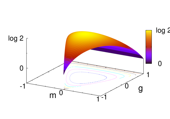
As a first application of the results presented in the previous section, we consider a model with $R=2$ and $\rho=1$ (i.e. the Hamiltonian is $\mathcal{H}=-h\sum_{i}s_{i}-j\sum_{i}s_{i}s_{i+1}$ where $h$ is the magnetic field and $j$ is the coupling). The only independent correlations are the one-body correlator, i.e. the magnetization $m\equiv g_{\{1\}}$, and the nearest-neighbour correlator $g\equiv g_{\{1,2\}}$. Using (10) the entropy is calculated as

$$s(m,g)=-\frac{1+2m+g}{4}\log\left(\frac{1+2m+g}{4}\right)-\frac{1-2m+g}{4}\log\left(\frac{1-2m+g}{4}\right)$$

$$-\frac{1-g}{2}\log\left(\frac{1-g}{4}\right)+\frac{1+m}{2}\log\left(\frac{1+m}{2}\right)+\frac{1-m}{2}\log\left(\frac{1-m}{2}\right)$$ (16)

which agrees with the expression obtained in mukamel2005 by combinatorial means. In figure 2 we plot the entropy: the convexity of $s$ guarantees to obtain the field and nearest-neighbour interaction in terms of $m$ and $g$. The system we have just described presents no phase transitions, apart from the zero temperature ones which occur at the border of the surface depicted in figure 2; in section VI we will see how the addition of a mean-field type interaction is easily included, making phase transitions possible. Interestingly on the lines $1\pm 2m+g=0$ the system is frustrated and our approach readily provides an expression for the ground state degeneracy. Differentiation of the entropy (IV) allows us to obtain the couplings, field $h\equiv j_{\{1\}}$ and nearest-neighbour interaction $j\equiv j_{\{1,2\}}$ conjugated to $m$ and $g$ respectively:

$$h= -\frac{\partial{s(m,g)}}{\partial m}=\frac{1}{2}\log\frac{(1-m)(1+2m+g)}{(1+m)(1-2m+g)}$$ (17)

$$j= -\frac{\partial{s(m,g)}}{\partial g}=\frac{1}{4}\log\frac{(1+2m+g)(1-2m+g)}{(1-g)^{2}}.$$ (18)

In Appendix A we examine this example ($R=2$ and $\rho=1$) and higher range ones ($R=3,4$ and $\rho=1$), explicitly checking the validity of the inversion formula (9) using the transfer matrix method.

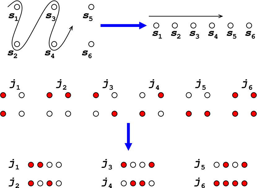
We will consider now a translationally invariant spin ladder with interaction among the nearest-neighbors of the same and other chain. For simplicity we will restrict ourselves to even interactions, i.e. in the Hamiltonian only terms containing an even number of spins enter. As shown explicitly in figure 2 this system may be mapped onto a chain system with $R=4$ and $\rho=2$, where the original interactions (allowed by symmetry) and the new ones are shown. In terms of our subset notation used in (3) the interaction parameters are defined as $j_{1}\equiv j_{\{1,2\}},j_{2}\equiv j_{\{1,3\}},j_{3}\equiv j_{\{1,4\}},j_{4}\equiv j_{\{2,3\}},j_{5}\equiv j_{\{2,4\}},j_{6}\equiv j_{\{1,2,3,4\}}$. This is easily generalized to ladders made up of more than two chains and higher interaction range, and thus our method is suited to treat general finite-range ladder systems.

We point out that the inversion formula allows to explicitly write the relation among the $j$’s and $g$’s while the transfer matrix approach, e.g. in the simple ladder system described above, already entails the solution of a fourth order algebraic equation.

IV.1 Nearest-neighbour and next-to-nearest-neighbour plus four-spin interactions

In this section we consider another simple example, in which nearest-neighbour and next-to-nearest-neighbour interactions are present together with a four-spin interaction: denoting the coefficients $j_{i,i+1}^{(2)}$, $j_{i,i+2}^{(2)}$ and $j_{i,i+1,i+2,i+3}^{(4)}$ by $j_{1}$, $j_{2}$ and $\lambda$ respectively, the Hamiltonian (1) reads

$$\mathcal{H}=-\sum_{i}\left(j_{1}s_{i}s_{i+1}+j_{2}s_{i}s_{i+2}+\lambda s_{i}s_{i+1}s_{i+2}s_{i+3}\right).$$ (19)

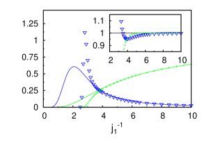
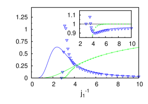
This Hamiltonian can be exactly treated in our framework; the case $\lambda=\;0$ (the $j_{1}-j_{2}$ model) is discussed in the Appendix. Here we aim at comparing approximate inverse Ising methods against exact results, focusing in particular on the low-correlation expansion (LCE) sessak2009 which is in the following compared with exact findings. We will use the LCE discussed in sessak2009 using as input a finite number of correlations, coherently with what is done in this work (notice that for the present case our method needs just four correlation functions in order to recover exactly the couplings); the maximal range of two-body correlators for the LCE is denoted by $R_{rec}$.

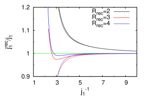
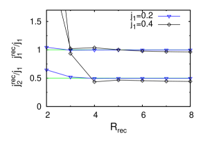
The LCE is discussed in sessak2009 to present an approximate technique for inverse Ising models having at most two-spin interactions: since Hamiltonian (1) has only two-spin interactions for $\lambda=0$, we present LCE results for the case $\lambda=0$ in the Appendix where we discuss the $j_{1}-j_{2}$ model in detail, presenting the explicit solution using the transfer matrix approach. As expected, for low temperatures (i.e. large couplings), the LCE breaks down and, as it can be seen in the right panel of figure 8, for moderate temperatures the expansion may settle to an incorrect value of the coupling as the range $R_{rec}$ is increased. In order to further test the performance of the LCE against exact results we present in figure 3 results for $\lambda=0$ and $\lambda=0.2j_{1}$: although the LCE is developed in sessak2009 for two-spin interactions (and the extension to treat multispin interactions is expected to be cumbersome), the LCE reconstructed two-spin couplings with $\lambda\neq 0$ may partially take into account the effect of the four-spin interaction. To test to what extent this occurs, we consider two observables, susceptibility and specific heat, calculated using the reconstructed couplings: the comparison with the exact results is in figure 3. As we can see in the left panel the specific heat is more sensitive than the susceptibility to reconstruction errors, even without four-spin interaction (i.e. $\lambda=0$). This may be traced back to this type of LCE inversion procedure which aims at reproducing two body correlators which in this model are required to calculate the susceptibility while the specific heat already contains averages of four body operators. Obviously the LCE, being not designed to infer models with multispin interaction, gives no hint on the value $\lambda$ but in the right panel of figure 3 we apply it for $\lambda=0.2$ in order to test how it can reproduce the considered observables anyway: we can see that the addition of such an operator reduce the temperature range where the observables are correctly reproduced. As noted above the specific heat is more subjected to errors than the susceptibility at contains higher-body operators. From numerical inspection we saw that the LCE rather well performs in the high temperature regime even for relatively large values of $\lambda$, but deviates from exact results at lower temperature even for small values of $\lambda$ as shown in figure 3.

Figure 3: Values for inverse susceptibility (green crosses) and specific heat (blue triangles) calculated with the LCE reconstructed couplings compared with the exact ones (full lines) as the inverse coupling $j_{1}$ is varied. The value $j_{2}/j_{1}$ is held fixed at the value $1$. The figure on the right includes the four-spin interaction whose coupling is fixed at the value $\lambda=0.2\;j_{1}$. The inset shows the ratio between the predicted values of specific heat and inverse susceptibility and the exact ones. Both figures are obtained keeping $R_{rec}=8$ correlation functions and using third order loop resummed expansion to reconstruct the couplings, as presented in sessak2009 .

V Exponential and power-law two-spin plus higher-spin couplings

Figure 4: Two examples of reconstructed values of the two-body couplings $j^{(2)}_{i,j}$ (empty symbols) and the values of the couplings really used to generate the correlations (filled circles) - the full line is a guide to the eye. The figures refers to Hamiltonian (20) with parameters $J_{0}=0.2$, $\xi=1.6$, $R_{max}=6,4$ (left) and $J_{0}=0.1$, $\xi=2.3$, $R_{max}=8,6$ (right).

Figure 5: Measured values of the correlations $g_{\mu}$ (top) and the inferred couplings $j_{\mu}$ (bottom) for the $\mu$’s allowed by translational symmetry (filled blue circles) and exact values (empty purple triangles). The black diamonds refer to LCE results obtained with the perturbative expansion up to third order sessak2009 . The figure at the bottom is a logarithmic plot of the absolute values of the $j_{\mu}$’s, while the inset gives for comparison the linear plot of the same $j_{\mu}$’s. The figures refer to Hamiltonian (20) with parameters $J_{0}=0.2$, $\xi=1.6$. The reconstruction range is $R_{max}=6$. In abscissa are reported the $\mu$’s denoting the various coupling and correlators with the subset notation introduced in section II, e.g. $g_{\{1\}}=\langle s_{1}\rangle$ is the correlation of the subset $\mu=\{1\}$, $g_{\{1,2,4\}}=\langle s_{1}s_{2}s_{4}\rangle$ is the correlation of the subset $\mu=\{1,2,4\}$ and so on.

In this section we consider examples where we cannot access the full knowledge of our system: our inversion procedure will therefore yield approximate results. First, we consider an Ising model with an exponentially decaying two-body interaction

$$H_{I}=-\sum_{(i,j)}j^{(2)}_{i,j}s_{i}s_{j},\;\quad j^{(2)}_{i,j}=J_{0}e^{-|i-j|/\xi}.$$ (20)

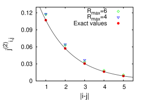
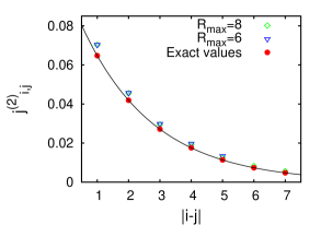
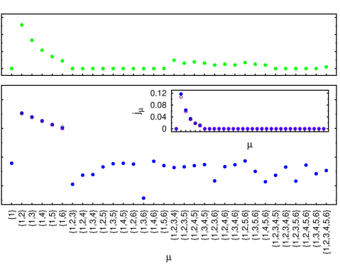
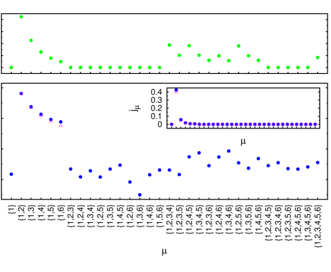
Since the interaction now is not formally of “finite range” i.e. it does not vanish for distances beyond a given value of $R$, the transfer matrix method is not viable (although we still may perform a finite-range scaling in the size of the transfer matrix uzelac1988 ; uzelac1989 ). The set of synthetic correlation functions is generated by a Monte Carlo method. Of course we will not record all of the correlation function, but we will fix a maximal range $R_{max}$, thus we will have to measure on the order of $2^{R_{max}}$ correlation functions. The results for such a reconstruction are shown in figure 4 for two values of the parameters. We see that the agreement improves as the value of $R_{max}$ is increased (at the expense of calculating a larger number of correlation functions). In figure 5 a full set of the correlations and inferred couplings is shown; if we look at the lower panel, the nonzero couplings are clearly singled out (even for a value of $R_{max}$ as low as $6$), thus our reconstruction procedure gives useful hints to build a faithful model of an unknown system. In figure 5 results obtained with the LCE are also reported: one sees that there is a good agreement for the considered value of the temperature between the LCE results and the findings obtained using our reconstruction procedure.

In order to test the procedure on a system with more-body couplings we consider the Hamiltonian

$$H_{II}=H_{I}-j_{\{1,2,4\}}\sum_{i}s_{i+1}s_{i+2}s_{i+4}-j_{\{1,3,4,5\}}\sum_{i}s_{i+1}s_{i+3}s_{i+4}s_{i+5}$$ (21)

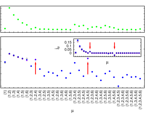
which includes three- and four-body interactions. As we see in figure 6, even in this case the reconstruction procedure gives useful hints on the couplings present in the system, although some of the inferred couplings, which were zero in the starting model, are predicted to be of comparable size to the nonzero ones (especially the $j_{\{1,2,3,4\}}$ coupling). This is due to the finite reconstruction range and to the, albeit small (indeed smaller than the symbols in the figures 5, 6, 7), errors in the determination of the correlation. This implies that in order to clearly distinguish the contribution of the different couplings, the correlation should be known with high accuracy. As for modeling purposes, this is not a problem since the values of the coupling obtained give rise to a set of correlations not distinguishable from the original one. For reference we also plot in figure 6 the results of the TAP equation approach developed in roudi2009 , which of course provides no information on the multispin couplings, but as far as one-body operators and two-body operators are concerned this approach at the temperature considered in figure 6 performs very well.

Finally we examine a model with power-law decay of the interaction

$$H_{III}=-\sum_{(i,j)}j^{(2)}_{i,j}s_{i}s_{j},\;\quad j^{(2)}_{i,j}=\frac{J_{0}}{|i-j|^{\alpha}}.$$ (22)

As can be seen in figure 7 (with $\alpha=3$), the results are good also in this case: it can be generally observed that the reconstructed interactions are higher than the exact ones, due to the fact that the interaction within the reconstruction range have to account for the interactions lying outside this range.

Figure 6: Same as figure 5 except for the black diamonds which are obtained with the TAP approach roudi2009 . The figures refer to Hamiltonian (21) with parameters $J_{0}=0.3$, $\xi=1.6$, $j_{\{1,2,4\}}=0.02$, $j_{\{1,3,4,5\}}=-0.03$. The reconstruction range is $R_{max}=6$. The arrows mark the multispin interactions.

Figure 7: Same as figure 5. Measured values of the correlations $g_{\mu}$ (top) and inferred couplings $j_{\mu}$ (bottom) for the power-law decaying Hamiltonian (22) with parameters $J_{0}=0.4$, $\alpha=3$. The reconstruction range is $R_{max}=6$.

VI Mean-field couplings

In this section we briefly discuss how our previous results can be used in presence of mean-field long-range interactions, showing that our inversion approach may be used on this class of systems. We consider a system with energy $e$ of general form, i.e. a non-linear function of the correlators. The number of couplings entering the energy $e$ should still equal the number of independent correlation functions in order to perform, at least in principle, the inversion procedure. Such an energy will be denoted by $e^{MF}(\{g_{\mu}\},\{j^{MF}_{m}\})$ where the index $m$ runs over the mean-field couplings.

By requiring the free energy $f^{MF}(\{g_{\mu}\},\{j^{MF}_{m}\})=e^{MF}(\{g_{\mu}\},\{j^{MF}_{m}\})-s(\{g_{\mu}\})$ to have a minimum when the ${g_{\mu}}$ are set to the known values will give the equations implicitly determining all the couplings, including the mean-filed ones $\{j^{MF}_{m}\}$. When the energy is differentiable these equations read

$$\frac{\partial e^{MF}(\{g_{\mu}\},\{j^{MF}_{m}\})}{\partial g_{\mu}}=\frac{\partial s(\{g_{\mu}\})}{\partial g_{\mu}}.$$ (23)

This set of equations will in general have multiple solutions or possibly no solutions at all. If more solutions are present the one (or ones) rendering the free energy minimal should be chosen. The points where the absolute minimum of the free energy branches or it changes discontinuously will signal a phase transition. As described in the section III some values of the couplings may be known in advance thus reducing the number of equations to be solved. Another possibility is that a function of the coupling is fixed; a notable example being the energy itself, corresponding to the microcanonical description of the system. We remark that in the class of models we consider all of these steps can be carried out exactly since the explicit form of entropy (10) is known.

As an example we may consider the first model examined in section IV ($R=2$, $\rho=1$) by adding mean-field two-body couplings. Instead of the energy $e(m,g)=-hm-jg$ (where $h=j_{\{1\}}$ and $j=j_{\{1,2\}}$ ) we will set $e=e^{MF}(m,g)=-j^{MF}m^{2}-jg$. The appearance of the nonlinear term $m^{2}$ in the energy is due to the presence of non-local mean-field operators in the spin Hamiltonian like $-j^{MF}/N\left(\sum_{i=1}^{N}s_{i}\right)^{2}$. It should be noted that such an operator is not uniquely defined, e.g. the operator

$$-\frac{j^{MF}}{\sum_{i=1}^{N}\frac{1}{i^{\alpha}}}\sum_{i,j}\frac{s_{i}s_{j}}{|i-j|^{\alpha}}\quad\left(0<\alpha<1\right)$$ (24)

and other Kac-rescaled nonextensive potentials give rise to the term $-j^{MF}m^{2}$ in the energy density at the thermodynamic limit when evaluated on a state with magnetization $m$ and nearest-neighbour correlation $g$ vollmayr-lee2001 . If we set $j=0$ we get the usual mean-field model, otherwise we obtain a model with competing mean-field and short-range coupling introduced by Kardar kardar1983 , exhibiting a complex phase diagram which shows nonequivalence between the canonical and microcanonical description mukamel2005 (for a review on inequivalence between ensembles and other issues concerning nonextensive systems see ruffo2009 ). As already observed the entropy of such a model within our approach is easily computed [see (IV)] and it could be generalized thus allowing one to treat one-dimensional models possessing multiple competing finite-range and mean-field interactions.

VII Conclusions

In this paper we presented the explicit solutions of the inverse Ising problem for a one-dimensional translational invariant model with arbitrary finite-range multispin interactions once a number $\sim 2^{R}$ (where $R$ is the range of the interactions) of independent correlations is known. When applied to unknown systems this method correctly detects arbitrary interactions; our results are then applied to systems with a range extending beyond the one set by maximum distance of the spins of the recorded correlation functions, giving useful hints on the interactions that should be kept in an effective model.

As an application, we reconstructed the couplings of chain Ising Hamiltonians having exponential or power-law two-spin plus three- or four-spin couplings. We also discussed the generalization of the method to ladders. Mean-field interactions can be also included in the framework, allowing us to describe systems exhibiting phase transitions. The presence of both finite-range (local) and mean-field (nonlocal) interactions can give rise to interesting competition effects greatly enhancing the descriptive power of the models we can exactly solve with our techniques. Our results provide then a theoretical laboratory where different approximate inverse Ising techniques can be benchmarked against the exact results obtained using our method: in the paper we performed such comparison is some illustrative examples.

The one-dimensional inverse Ising problem we have solved in the present paper is analogous to what may be called the inverse Markov chain problem: given a specific set of correlations at equilibrium, find the corresponding transition rates. The two inversion (Ising and Markov) problems are related since it is possible to associate an Ising model to an equilibrium Markov Ising chain with finite memory in full generality: to show it, for definiteness let us consider Ising variables (although extensions to other discrete state spaces is straightforward). The finite-range $R$ in our solution of the inverse one-dimensional Ising problem is the counterpart of the finite memory in the inverse Markov problem: let the state of the next $\rho$ spins be ruled by the state of the preceding $R-\rho$ spins. We put the new spins on the right side of the old ones: the time of the Markov process is increasing from left to right. The correlations impose constraints on the transition rates: it turns out that the number of independent correlations required to solve the inverse Markov problem is the same as the number needed to solve the (related) inverse Ising problem in one dimension of range $R$ and period $\rho$, i.e. the number of independent correlations is $2^{R}-2^{R-\rho}$. Adapting the procedure discussed in section III which lead to (12) it is possible to compute the transition rates from the state $\tau_{R-\rho}$ of $R-\rho$ spins to the state $\theta_{\rho}$ of $\rho$ spins. These transitions are given by

$$w_{\tau_{R-\rho}\rightarrow\theta_{\rho}}=\frac{p(\eta_{R})}{p(\tau_{R-\rho})},$$ (25)

where the $p$’s are calculated according to formula (12) where the input correlations $\{g_{\mu}\}$’s are plugged in, and $\eta_{R}$ is the configuration of $R$ spins obtained by juxtaposing the states $\tau_{R-\rho}$ (on the left) and $\theta_{\rho}$ (on the right). The transition matrix obtained this way is a $2^{R-\rho}$ by $2^{\rho}$ matrix; in order to have a square matrix we have to fold more steps of the the transition matrix until we obtain the probability to go from a set of $\max(R-\rho,\rho)$ to the next $\max(R-\rho,\rho)$ spins gori_future . The transition matrix satisfies detailed balance by construction, therefore this is a reversible Markov chain. This mapping has already been worked out in a discrete different form in vanderstraeten2009 where the connection to discrete statistical models is also discussed.

According to the previous discussion, we may thus associate an Ising model to the an equilibrium Markov Ising chain with finite memory in full generality, allowing us to treat systems where one direction (typically time) is singled out. As a possible example deserving future investigation one could consider time-series of financial data and try to estimate with the procedure discussed before the transition probabilities of the associated guessed Markov chain in order to test the validity of such a description. It is intended - in order to apply the previous results - that the analyzed data should be discretized on a timescale such that nontrivial correlations occur, and that the whole time of observation is such that the system can be reliably considered at equilibrium. Obviously a way to encode significant information in an Ising variable has to be devised, being this in general a nontrivial task; for example, we may think of “up” and “down” spin corresponding to a price raise or lowering respectively. The next step would be to analyze the correlations among different time-series of data to determine if and how correlations among different stocks occur. For example the Ising ladder system depicted in figure 2 may reproduce the correlations among two stocks whose state depends on the value of the other stock at the same timestep and on the value of the same or other stock at the previous timestep (for simplicity, in figure 2 odd interactions are not depicted). E.g., it should be noted that the inclusion of the interaction dubbed $j_{6}$ in figure 2 may reproduce some kind of nontrivial many-body interaction among the stocks. Extending the number of chains in the ladder system and/or the range allows us to treat larger sets of stocks with longer correlations in time.

We think that studying stationary time-series of correlated data using the techniques presented in this paper (and as well the mapping onto Markov chains discussed in this section) will be an interesting subject of future research. In perspective, one could apply the method here discussed to datasets and/or statistical mechanics models which are supposed to be described by effective one-dimensional Ising chains near the thermodynamical limit. To this aim, one should address in the future a treatment of the case where large errors in the measured correlation functions are present and/or some of the correlations are missing; our exact result could be a good starting point to move in that direction. Next, our results could be extended in higher dimensional cases (where of course one does not expect to find closed formulas), hierarchical or tree-like models. Some preliminary results in the two dimensional case seem to indicate that this approach leads to equations resembling the Dobrushin-Lanford-Ruelle ones dobrushin1969 ; lanford1969 . Another interesting direction could be to use the a renormalization group approach on the correlation functions, in order to study how the couplings determined by correlations at some scale $R$ are related to the ones computed at a larger scale $R^{\prime}$.

Acknowlegments: We wish to thank I. Mastromatteo and M. Marsili for many very useful discussions. This work has been supported by the grants INSTANS (from ESF) and 2007JHLPEZ (from MIUR).

Appendix A Transfer Matrices

In this Appendix we work out the transfer matrix for the general translational invariant ($\rho=1$) Ising model with range $R=2,3,4$ and we check that the results obtained analytically and numerically with the transfer matrix formalism are fully consistent with the predictions of the formula (10).

We start by briefly recalling the method (see e.g. yeomans1992 ). In general the transfer matrix $\mathbf{T}$ is built by identifying the $2^{B}$ states of a block of spins $B$ with independent and orthogonal vector of a space of dimension $2^{B}$ such that the matrix elements of $\mathbf{T}$ are

$$\langle a|\mathbf{T}|b\rangle=e^{-\mathcal{H}_{int}(a)-\mathcal{H}_{ext}(a,b)},$$ (26)

where $\mathcal{H}_{ext}(a,b)$ is the interaction energy among two consecutive blocks of spins $a$ and $b$ ($a$ is placed to the left of $b$), $\mathcal{H}_{int}(a)$ is the interaction energy among the spins belonging to the same block. The vector corresponding to the spin state $a$ is denoted, using the ket notation, by $|a\rangle$. The size of the blocks $B$ has to be chosen according to the range and size of the unit cell $\rho$ of the system in order to have all of the interaction terms contained in $\mathcal{H}_{int}$ or $\mathcal{H}_{ext}$. The partition function of the system of size $N$ is simply given by $\mathcal{Z}_{N}=\mathrm{Tr}(\mathbf{T}^{N/B})$ so that in the infinite size limit the free energy per unit cell may be written in terms of the largest eigenvalue $\lambda_{max}$ of $\mathbf{T}$:

$$f=-\frac{1}{B/\rho}\log\lambda_{max}.$$ (27)

The existence and unicity of $\lambda_{max}$ is guaranteed by Perron-Frobenius theorem, being all elements of $\mathbf{T}$ strictly positive (for nonvanishing temperature). The correlation functions may be obtained just by differentiation of the free energy $f$.

We start with the simple example of $R=2$ which has been worked out in section IV. The two independent couplings will be denoted as usual by $j_{\{1\}}=h$ (magnetic field) and $j_{\{1,2\}}=j$ (nearest-neighbour coupling). The $2$ by $2$ transfer matrix $\mathbf{T}$, with the states identification $|\uparrow\rangle=(1,0)$ and $|\downarrow\rangle=(0,1)$, reads

$$\mathbf{T}=\left(\begin{array}[]{cc}e^{h+j}&e^{h-j}\\ e^{-h-j}&e^{-h+j}\end{array}\right).$$ (28)

The free energy is then given by

$$f(h,j)=-\log\left[e^{j}\cosh h+\sqrt{e^{2j}\cosh^{2}h-2\sinh(2j)}\right].$$ (29)

Differentiating $f(h,j)$ with respect to $h$ and $j$ gives the magnetization $m$ and the nearest-neighbour correlation $g$ respectively:

$$m= -\frac{\partial{f(h,j)}}{\partial h}=\frac{e^{j}\sinh h}{\sqrt{e^{2j}\cosh^{2}h-2\sinh(2j)}}$$ (30)

$$g= -\frac{\partial{f(h,j)}}{\partial j}=\coth(2j)-\frac{\cosh h}{\sinh(2j)\sqrt{1+e^{4j}\sinh^{2}h}}.$$ (31)

The inversion of the above formulas with respect to $h$ and $j$ yields the expressions (17).

Now we consider a model with only even interactions and range $R=3$, i.e. containing the coupling $j_{1}=j_{\{1,2\}}$ and $j_{2}=j_{\{1,3\}}$ which we dub $j_{1}-j_{2}$ model: the corresponding Hamiltonian is given by (19) with $\lambda=0$. This model may be mapped onto the previous example ($R=2$, $\rho=1$) by introducing “kink” variables $s_{i}s_{i+1}$ with the identifications $j_{1}=h$, $j_{2}=j$ (we do not report the corresponding results). In figure 8 we plot the couplings reconstructed according to the low-coupling expansion (LCE) introduced in sessak2009 against the exact results which can be found by the method discussed in this paper or by the transfer matrix approach. The LCE allows to infer the magnetic fields and the two-body couplings from the two-body correlators and magnetizations. In sessak2009 the LCE has been carried out, in the zero field case, up to seventh order in the correlations with loop resummation. We have used the LCE as both the order of the expansion and the number of correlation function we assume to know are increased. The maximal range of two-body correlations which are used as input is denoted by $R_{rec}$. In figure 8 we depict the reconstructed couplings $j_{1}^{rec}$, $j_{2}^{rec}$ and the exact ones for different values of $R_{rec}$. The ratio $j_{1}/j_{2}$ is kept fixed, thus $j_{1}$ serves as inverse temperature. As expected as the temperature is lowered the agreement gets worse, and it may be noticed that the inclusion of higher order terms in this case does not significantly improve the performance of the inversion: as one can see, the lower order results depicted in the left panel of figure 8 is more reliable at lower temperatures (this is the reason why in figure 3 we employed the third order LCE). In the right panel of figure 8 we can see how the the increase of $R_{rec}$ improves the quality of the inversion but beyond a given range the reconstructed couplings $j_{1,2}^{rec}$ settle to a value which, in the lower temperature case examined, deviates from the exact one.

Figure 8: On the left the ratio between the exact and reconstructed value of the nearest-neighbour coupling in terms of $j_{1}$. The various lines denote how many correlation functions are kept in the reconstruction formulas as indicated. The continuous and dotted line refer respectively to the third and seventh order in the LCE of sessak2009 (including the loop contributions). On the right the ratio of reconstructed $j^{rec}_{1}$ (above), $j^{rec}_{2}$ (below) and the exact value of $j_{1}$ in terms of the reconstruction range $R_{rec}$ are shown. Only the result for the seventh order LCE is shown. In both figures the green straight lines are the exact values and the nearest-neighbour coupling $j_{2}$ is set to the half of $j_{1}$.

We move on to the next example, the $R=3$ case with no restriction on the symmetry of the couplings. Identifying the states as $|\uparrow\uparrow\rangle=(1,0,0,0)$, $|\uparrow\downarrow\rangle=(0,1,0,0)$, $|\downarrow\uparrow\rangle=(0,0,1,0)$, $|\downarrow\downarrow\rangle=(0,0,0,1)$ and the couplings as $j_{\{1\}}=j_{1}$, $j_{\{1,2\}}=j_{2}$, $j_{\{1,3\}}=j_{3}$, $j_{\{1,2,3\}}=j_{4}$, the transfer matrix reads

$$\mathbf{T}=\left(\begin{array}[]{cccc}e^{2j_{1}+2j_{2}+2j_{3}+2j_{4}}&e^{2j_{1}-2j_{4}}&e^{2j_{1}+2j_{2}}&e^{2j_{1}-2j_{3}}\\ 1&e^{-2j_{2}+2j_{3}}&e^{-2j_{3}-2j_{4}}&e^{-2j_{2}+2j_{4}}\\ e^{-2j_{2}-2j_{4}}&e^{-2j_{3}+2j_{4}}&e^{-2j_{2}+2j_{3}}&1\\ e^{-2j_{1}-2j_{3}}&e^{-2j_{1}+2j_{2}}&e^{-2j_{1}+2j_{4}}&e^{-2j_{1}+2j_{2}+2j_{3}-2j_{4}}.\end{array}\right)$$ (32)

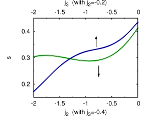
Proceeding as before, we can obtain the entropy and correlation functions. The comparison between the resulting obtained findings and our inversion formula are shown in the left panel of figure 9. The plot shows the numerically calculated entropy and the analytical one (10) where the numerical correlations are plugged in, for some values of the coupling constants. The entropy in this case is given by the expression (the subscripts in the $g$’s just indicate to which coupling they are conjugated):

$$s(g_{1},g_{2},g_{3},g_{4})=-\frac{1+g_{1}-g_{3}-g_{4}}{4}\log\left(\frac{1+g_{1}-g_{3}-g_{4}}{8}\right)-\frac{1+g_{1}-2g_{2}+g_{3}-g_{4}}{8}\log\left(\frac{1+g_{1}-2g_{2}+g_{3}-g_{4}}{8}\right)$$

$$-\frac{1-3g_{1}+2g_{2}+g_{3}-g_{4}}{8}\log\left(\frac{1-3g_{1}+2g_{2}+g_{3}-g_{4}}{8}\right)-\frac{1-g_{1}-g_{3}+g_{4}}{4}\log\left(\frac{1-g_{1}-g_{3}+g_{4}}{8}\right)$$

$$-\frac{1-g_{1}-2g_{2}+g_{3}+g_{4}}{8}\log\left(\frac{1-g_{1}-2g_{2}+g_{3}+g_{4}}{8}\right)-\frac{1+3g_{1}+2g_{2}+g_{3}+g_{4}}{8}\log\left(\frac{1+3g_{1}+2g_{2}+g_{3}+g_{4}}{8}\right)$$

$$+\frac{1-g_{2}}{2}\log\left(\frac{1-g_{2}}{4}\right)+\frac{1-2g_{1}+g_{2}}{4}\log\left(\frac{1-2g_{1}+g_{2}}{4}\right)+\frac{1+2g_{1}+g_{2}}{4}\log\left(\frac{1+2g_{1}+g_{2}}{4}\right).$$

As a last case we consider a translation invariant chain with range $R=4$: identifying the states as $|\uparrow\uparrow\uparrow\rangle=(1,0,0,0,0,0,0,0)$, $|\uparrow\uparrow\downarrow\rangle=(0,1,0,0,0,0,0,0)$, $|\uparrow\downarrow\uparrow\rangle=(0,0,1,0,0,0,0,0)$, $|\uparrow\downarrow\downarrow\rangle=(0,0,0,1,0,0,0,0)$, $|\downarrow\uparrow\uparrow\rangle=(0,0,0,0,1,0,0,0)$, $|\downarrow\uparrow\downarrow\rangle=(0,0,0,0,0,1,0,0)$, $|\downarrow\downarrow\uparrow\rangle=(0,0,0,0,0,0,1,0)$, $|\downarrow\downarrow\downarrow\rangle=(0,0,0,0,0,0,0,1)$ and the couplings as $j_{\{1\}}=j_{1}$, $j_{\{1,2\}}=j_{2}$, $j_{\{1,3\}}=j_{3}$, $j_{\{1,4\}}=j_{4}$, $j_{\{1,2,3\}}=j_{5}$, $j_{\{1,2,4\}}=j_{6}$, $j_{\{1,3,4\}}=j_{7}$, $j_{\{1,2,3,4\}}=j_{8}$, the $8$ by $8$ transfer matrix reads:

$$\mathbf{T} =\left(\begin{array}[]{cc}\mathbf{T}_{1}&\mathbf{T}_{2}\\ \mathbf{T}_{3}&\mathbf{T}_{4}\\ \end{array}\right)$$ (35)

where the $4\times 4$ matrices $\mathbf{T}_{1},\cdots,\mathbf{T}_{4}$ are

$$\mathbf{T}_{1} =\left(\begin{array}[]{cccc}e^{3j_{1}+3j_{2}+3j_{3}+3j_{4}+3j_{5}+3j_{6}+3j_{7}+3j_{8}}&e^{3j_{1}+j_{2}+j_{3}+j_{4}-j_{5}-j_{6}-j_{7}-3j_{8}}&e^{3j_{1}+3j_{2}+j_{3}+j_{4}+j_{5}+j_{6}-j_{7}-j_{8}}&e^{3j_{1}+j_{2}-j_{3}-j_{4}+j_{5}-3j_{6}-j_{7}+j_{8}}\\ e^{j_{1}+j_{2}+j_{3}+j_{4}+j_{5}+j_{6}+j_{7}+j_{8}}&e^{j_{1}-j_{2}-j_{3}+3j_{4}-3j_{5}+j_{6}+j_{7}-j_{8}}&e^{j_{1}+j_{2}-j_{3}-j_{4}-j_{5}-j_{6}-3j_{7}-3j_{8}}&e^{j_{1}-j_{2}-3j_{3}+j_{4}-j_{5}-j_{6}+j_{7}+3j_{8}}\\ e^{j_{1}-j_{2}+j_{3}+j_{4}-j_{5}-j_{6}+j_{7}-j_{8}}&e^{j_{1}-3j_{2}+3j_{3}-j_{4}-j_{5}-j_{6}+j_{7}+j_{8}}&e^{j_{1}-j_{2}-j_{3}+3j_{4}-3j_{5}+j_{6}+j_{7}-j_{8}}&e^{j_{1}-3j_{2}+j_{3}+j_{4}+j_{5}+j_{6}-3j_{7}+j_{8}}\\ e^{-j_{1}+j_{2}-j_{3}-j_{4}+j_{5}+j_{6}-j_{7}+j_{8}}&e^{-j_{1}-j_{2}+j_{3}+j_{4}+j_{5}-3j_{6}+3j_{7}-j_{8}}&e^{-j_{1}+j_{2}-3j_{3}+j_{4}-j_{5}+3j_{6}-j_{7}+j_{8}}&e^{-j_{1}-j_{2}-j_{3}+3j_{4}+3j_{5}-j_{6}-j_{7}-j_{8}}\end{array}\right)$$ (40)

$$\mathbf{T}_{2} =\left(\begin{array}[]{cccc}e^{3j_{1}+3j_{2}+3j_{3}+j_{4}+3j_{5}+j_{6}+j_{7}+j_{8}}&e^{3j_{1}+j_{2}+j_{3}-j_{4}-j_{5}+j_{6}-3j_{7}-j_{8}}&e^{3j_{1}+3j_{2}+j_{3}-j_{4}+j_{5}-j_{6}+j_{7}+j_{8}}&e^{3j_{1}+j_{2}-j_{3}-3j_{4}+j_{5}-j_{6}+j_{7}-j_{8}}\\ e^{j_{1}+j_{2}+j_{3}-j_{4}+j_{5}-j_{6}-j_{7}-j_{8}}&e^{j_{1}-j_{2}-j_{3}+j_{4}-3j_{5}+3j_{6}-j_{7}+j_{8}}&e^{j_{1}+j_{2}-j_{3}-3j_{4}-j_{5}-3j_{6}-j_{7}-j_{8}}&e^{j_{1}-j_{2}-3j_{3}-j_{4}-j_{5}+j_{6}+3j_{7}+j_{8}}\\ e^{j_{1}-j_{2}+j_{3}-j_{4}-j_{5}-3j_{6}-j_{7}-3j_{8}}&e^{j_{1}-3j_{2}+3j_{3}-3j_{4}-j_{5}+j_{6}-j_{7}+3j_{8}}&e^{j_{1}-j_{2}-j_{3}+j_{4}-3j_{5}-j_{6}+3j_{7}+j_{8}}&e^{j_{1}-3j_{2}+j_{3}-j_{4}+j_{5}+3j_{6}-j_{7}-j_{8}}\\ e^{-j_{1}+j_{2}-j_{3}-3j_{4}+j_{5}-j_{6}-3j_{7}-j_{8}}&e^{-j_{1}-j_{2}+j_{3}-j_{4}+j_{5}-j_{6}+j_{7}+j_{8}}&e^{-j_{1}+j_{2}-3j_{3}-j_{4}-j_{5}+j_{6}+j_{7}+3j_{8}}&e^{-j_{1}-j_{2}-j_{3}+j_{4}+3j_{5}+j_{6}+j_{7}-3j_{8}}\end{array}\right)$$ (45)

$$\mathbf{T}_{3} =\left(\begin{array}[]{cccc}e^{j_{1}-j_{2}-j_{3}+j_{4}-3j_{5}-j_{6}-j_{7}-3j_{8}}&e^{j_{1}+j_{2}-3j_{3}-j_{4}+j_{5}-j_{6}-j_{7}+3j_{8}}&e^{j_{1}-j_{2}+j_{3}-j_{4}-j_{5}+j_{6}-j_{7}+j_{8}}&e^{j_{1}+j_{2}-j_{3}-3j_{4}-j_{5}+j_{6}+3j_{7}-j_{8}}\\ e^{-j_{1}-3j_{2}+j_{3}-j_{4}-j_{5}-3j_{6}+j_{7}-j_{8}}&e^{-j_{1}-j_{2}-j_{3}+j_{4}+3j_{5}+j_{6}-3j_{7}+j_{8}}&e^{-j_{1}-3j_{2}+3j_{3}-3j_{4}+j_{5}-j_{6}+j_{7}+3j_{8}}&e^{-j_{1}-j_{2}+j_{3}-j_{4}+j_{5}+3j_{6}+j_{7}-3j_{8}}\\ e^{-j_{1}-j_{2}-3j_{3}-j_{4}+j_{5}-j_{6}-3j_{7}+j_{8}}&e^{-j_{1}+j_{2}-j_{3}-3j_{4}+j_{5}+3j_{6}+j_{7}-j_{8}}&e^{-j_{1}-j_{2}-j_{3}+j_{4}+3j_{5}-3j_{6}+j_{7}+j_{8}}&e^{-j_{1}+j_{2}+j_{3}-j_{4}-j_{5}+j_{6}+j_{7}-j_{8}}\\ e^{-3j_{1}+j_{2}-j_{3}-3j_{4}-j_{5}+j_{6}-j_{7}-j_{8}}&e^{-3j_{1}+3j_{2}+j_{3}-j_{4}-j_{5}+j_{6}-j_{7}+j_{8}}&e^{-3j_{1}+j_{2}+j_{3}-j_{4}+j_{5}-j_{6}+3j_{7}-j_{8}}&e^{-3j_{1}+3j_{2}+3j_{3}+j_{4}-3j_{5}-j_{6}-j_{7}+j_{8}}\end{array}\right)$$ (50)

$$\mathbf{T}_{4} =\left(\begin{array}[]{cccc}e^{j_{1}-j_{2}-j_{3}+3j_{4}-3j_{5}+j_{6}+j_{7}-j_{8}}&e^{j_{1}+j_{2}-3j_{3}+j_{4}+j_{5}-3j_{6}+j_{7}+j_{8}}&e^{j_{1}-j_{2}+j_{3}+j_{4}-j_{5}+3j_{6}-3j_{7}-j_{8}}&e^{j_{1}+j_{2}-j_{3}-j_{4}-j_{5}-j_{6}+j_{7}+j_{8}}\\ e^{-j_{1}-3j_{2}+j_{3}+j_{4}-j_{5}-j_{6}+3j_{7}+j_{8}}&e^{-j_{1}-j_{2}-j_{3}+3j_{4}+3j_{5}-j_{6}-j_{7}-j_{8}}&e^{-j_{1}-3j_{2}+3j_{3}-j_{4}+j_{5}+j_{6}-j_{7}+j_{8}}&e^{-j_{1}-j_{2}+j_{3}+j_{4}+j_{5}+j_{6}-j_{7}-j_{8}}\\ e^{-j_{1}-j_{2}-3j_{3}+j_{4}+j_{5}+j_{6}-j_{7}+3j_{8}}&e^{-j_{1}+j_{2}-j_{3}-j_{4}+j_{5}+j_{6}+3j_{7}-3j_{8}}&e^{-j_{1}-j_{2}-j_{3}+3j_{4}+3j_{5}-j_{6}-j_{7}-j_{8}}&e^{-j_{1}+j_{2}+j_{3}+j_{4}-j_{5}-j_{6}-j_{7}+j_{8}}\\ e^{-3j_{1}+j_{2}-j_{3}-j_{4}-j_{5}+3j_{6}+j_{7}+j_{8}}&e^{-3j_{1}+3j_{2}+j_{3}+j_{4}-j_{5}-j_{6}+j_{7}-j_{8}}&e^{-3j_{1}+j_{2}+j_{3}+j_{4}+j_{5}+j_{6}+j_{7}-3j_{8}}&e^{-3j_{1}+3j_{2}+3j_{3}+3j_{4}-3j_{5}-3j_{6}-3j_{7}+3j_{8}}\end{array}\right)$$ (55)

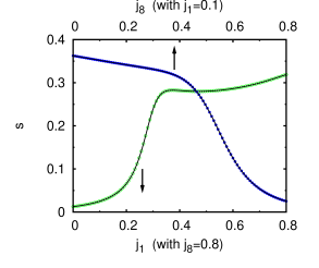
Results are shown in figure 9 (we do not write down the entropy for this case). By inspecting figure 9 we find that the agreement between the two approaches is complete. We do not report here the other checks we performed for higher values of $R$.

Figure 9: Entropy for some values of the coupling constants: $j_{1}=-0.1,j_{4}=-0.8$ (left) for the transfer matrix (32) and $j_{2}=0.2,j_{3}=-0.3,j_{4}=0.4,j_{5}=-0.5,j_{6}=0.6,j_{7}=-0.7$ (right) for the transfer matrix (35). The values of the remaining couplings are specified on the $x$-axes of the plots. The arrows point to the relevant $x$-axis. The continuous curves are obtained by numerical calculation, while the dots are calculated by means of (10).

References

- (1) J. V. Beck and K. J. Arnold, Parameter estimation in engineering and science, Wiley, New York (1977).
- (2) B. Bezruchko and D. Smirnov, Extracting knowledge from time series: an introduction to nonlinear empirical modeling, Springer, Berlin Heidelberg (2010).
- (3) A.-L. Barabási, Linked: The New Science of Networks, Perseus, Cambridge, MA (2002).
- (4) B. P. Carlin and S. Chib, J. Royal Stat. Soc. Series B 57, 473 (1995).
- (5) D. McKay, Information Theory, Inference, and Learning Algorithms, Cambridge University Press, Cambridge (2003).
- (6) E. Schneidman, M. J. Berry II, R. Segev, and W. Bialek, Nature 440, 1007 (2006).
- (7) S. Cocco, S. Leibler, and R. Monasson, Proc. Natl. Acad. Sci. U.S.A. 106, 14058 (2009).
- (8) S. Cocco and R. Monasson, Phys. Rev. Lett. 106, 090601 (2011).
- (9) R. N. Mantegna and H. E. Stanley, An Introduction to Econophysics, Cambridge University Press, Cambridge (2000).
- (10) G. Mussardo, Statistical Field Theory, Oxford University Press, Oxford (2010).
- (11) J. Villain , R. Bidaux, J.-P. Carton, and R. Conte, J. Phys. (Paris) 41, 1263 (1980).
- (12) P. Chandra, P. Coleman, and A. I. Larkin, Phys. Rev. Lett. 64, 88 (1990).
- (13) T. Horiguchi and T. Morita, J. Phys. Soc. Jap. 59, 888 (1990).
- (14) C. Weber, L. Capriotti, G. Misguich, F. Becca, M. Elhajal, and F. Mila, Phys. Rev. Lett. 91, 177202 (2003).
- (15) W. Krauth, Statistical mechanics: algorithms and computations, Oxford University Press, Oxford (2006).
- (16) E. Marinari and V. Van Kerrebroeck, J. Stat. Mech. P02008 (2010).
- (17) Y. Roudi, J. Tyrcha and J. Hertz, Phys. Rev. E 79, 51915 (2009).
- (18) V. Sessak, Ph. D. thesis, Université Pierre et Marie Curie, Paris (2011).
- (19) V. Sessak and R. Monasson, J. Phys. A: Math. Theor. 42, 055001 (2009).
- (20) B. H. Zimm and J. K. Bragg, J. Chem. Phys. 31, 526 (1959).
- (21) S. Lifson and A. Roig (1961), J. Chem. Phys. 34, 1963 (1961).
- (22) J. Schreck and J. Yuan, Phys. Rev. E 81, 061919 (2010).
- (23) R. Durbin, S. R. Eddy, A. Krogh, and G. Mitchison, Probabilistic models of proteins and nucleic acids, Cambridge University Press (2002).
- (24) K. Uzelac and Z. Glumac J. Phys. A: Math. Gen. 21, L421 (1988).
- (25) Z. Glumac and K. Uzelac J. Phys. A: Math. Gen. 22, 4439 (1989).
- (26) D. J. Thouless, Phys. Rev. 187, 732 (1969).
- (27) J. M. Kosterlitz, Phys. Rev. Lett. 37, 1577 (1976).
- (28) J. L. Cardy, J. Phys. A 14, 1407 (1981).
- (29) E. Luijten and H. Messingfeld, Phys. Rev. Lett. 86, 5305 (2001).
- (30) M. E. Fisher, S.-K. Ma, and B. G. Nickel, Phys. Rev. Lett. 29, 917 (1972).
- (31) H. Blöte and E. Luijten, Phys. Rev. B 56, 8945 (1997).
- (32) K. Binder and E. Luijten, Phys. Rep. 344, 179 (2001).
- (33) H. P. Büchler, A. Micheli, and P. Zoller, Nature Phys. 3, 726 (2007).
- (34) I. Mastromatteo and M. Marsili, in preparation.
- (35) D. Mukamel, S. Ruffo, and N. Schreiber, Phys. Rev. Lett. 95, 240604 (2005).
- (36) B. P. Vollmayr-Lee and E. Luijten, Phys. Rev. E 63, 031108 (2001).
- (37) M. Kardar, Phys. Rev. Lett. 51, 523 (1983); Phys. Rev. B 28, 244 (1983).
- (38) A. Campa, T. Dauxois, and S. Ruffo, Phys. Rep. 480, 57 (2009).
- (39) G. Gori and A. Trombettoni, in preparation.
- (40) E. Van der Straeten, Entropy 11, 867 (2009)
- (41) R. L. Dobrushin, Theory Prob. Appl. 13, 197 (1969).
- (42) O. E. Lanford III and D. Ruelle, Commun. Math. Phys. 13, 194 (1969).
- (43) J. M. Yeomans, Statistical mechanics of phase transitions, Clarendon Press, Oxford (1992).