Convergence of gradient-based algorithms for the Hartree-Fock equations

Abstract.

The numerical solution of the Hartree-Fock equations is a central problem in quantum chemistry for which numerous algorithms exist. Attempts to justify these algorithms mathematically have been made, notably in [5], but, to our knowledge, no complete convergence proof has been published. In this paper, we prove the convergence of a natural gradient algorithm, using a gradient inequality for analytic functionals due to Łojasiewicz [15]. Then, expanding upon the analysis of [5], we prove convergence results for the Roothaan and Level-Shifting algorithms. In each case, our method of proof provides estimates on the convergence rate. We compare these with numerical results for the algorithms studied.

1. Introduction

In quantum chemistry, the Hartree-Fock method is one of the simplest approximations of the electronic structure of a molecule. By assuming minimal correlation between the $N$ electrons, it reduces Schrödinger’s equation, a linear partial differential equation on $\mathbb{R}^{3N}$, to the Hartree-Fock equations, a system of $N$ coupled nonlinear equations on $\mathbb{R}^{3}$. This approximation makes it much more tractable numerically. It is used both as a standalone description of the molecule and as a starting point for more advanced methods, such as the Møller-Plesset perturbation theory, or multi-configuration methods. Mathematically, the Hartree-Fock method leads to a coupled system of nonlinear integro-differential equations, which are discretized by expanding the solution on a finite Galerkin basis. The resulting nonlinear algebraic equations are then solved iteratively, using a variety of algorithms, the convergence of which is the subject of this work.

The mathematical structure of the Hartree-Fock equations was investigated in the 70’s, culminating in the proof of the existence of solutions by Lieb and Simon[13], later generalized by Lions[14]. On the other hand, despite their ubiquitous use in computational chemistry, the convergence of the various algorithms used to solve them is still poorly understood. A major step forward in this direction is the recent work of Cancès and Le Bris[5]. Using the density matrix formulation, they provided a mathematical explanation for the oscillatory behavior observed in the simplest algorithm, the Roothaan method, and proposed the Optimal Damping Algorithm (ODA), a new algorithm inspired directly by the mathematical structure of the constraint set[4]. This algorithm was designed to decrease the energy at each step, and linking the energy decrease to the difference of iterates allowed the authors to prove that this algorithm “numerically converges” in the weak sense that $\mathinner{\!\left\lVert D_{k}-D_{k-1}\right\rVert}\to 0$. In addition, the algorithm numerically converges towards an Aufbau solution[7]. This, to our knowledge, is the strongest convergence result available for an algorithm to solve the Hartree-Fock equations.

However, this is still mathematically unsatisfactory, as it does not guarantee convergence, and merely prohibits fast divergence. The difficulty in proving convergence of the algorithms used to solve the Hartree-Fock equations lies in the lack of understanding of the second-order properties of the energy functional (for instance, there are no local uniqueness results available). In other domains, the convergence of gradient-based methods has been established using the Łojasiewicz inequality for analytic functionals[15] (see for instance [18, 10]). This method of proof has the advantage of not requiring any second-order information.

In this paper, we use a gradient descent algorithm to solve the Hartree-Fock equations. This algorithm builds upon ideas from differential geometry[8] and the various projected gradient algorithms used in the context of quantum chemistry[6, 16, 1]. To our knowledge, this particular algorithm has never been applied to the Hartree-Fock equations. Although it lacks the sophistication of modern minimization methods (for instance, see the trust region methods of [9] and [11]), it is the most natural generalization of the classical gradient descent, and, as such, the simplest one to analyze mathematically. For this algorithm, following the method of [18], we prove convergence, and obtain explicit estimates on the convergence rate. We also apply the method to the widely used Roothaan and Level-Shifting algorithms, effectively linking these fixed-point algorithms to gradient methods.

The structure of this paper is as follows. We first introduce the Hartree-Fock problem in the mathematical setting of density matrices and prove a Łojasiewicz inequality on the constrained parameter space. We then introduce the gradient algorithm, and prove some estimates. We show the convergence and obtain convergence rates for this algorithm, then extend our method to the Roothaan and Level-Shifting algorithm, using an auxiliary energy functional following [5]. We finally test all these results numerically and compare the convergence of the algorithms.

2. Setting

We are concerned with the numerical solution of the Hartree-Fock equations. We will consider for simplicity of notation the spinless Hartree-Fock equations, where each orbital $\phi_{i}$ is a function in $L^{2}(\mathbb{R}^{3},\mathbb{R})$, although our results are easily transposed to other variants such as General Hartree-Fock (GHF) and Restricted Hartree-Fock (RHF).

In this paper, we consider a Galerkin discretization space with finite orthonormal basis $(\chi_{i})_{i=1\dots N_{b}}$. In this setting, the orbitals $\phi_{i}$ are expanded on this basis, and the operators we consider are $N_{b}\times N_{b}$ matrices. This finite dimension hypothesis is crucial for our results, and we comment on it in the conclusion.

The Hartree-Fock problem consists in minimizing the total energy of a N-body system. We describe the mathematical structure of the energy functional and the minimization set, and introduce a natural gradient descent to solve this problem numerically.

2.1. The energy

We consider the quantum N-body problem of $N$ electrons in a potential $V$ (in most applications, $V$ is the Coulombic potential created by a molecule or atom). In the spinless Hartree-Fock model, this problem is simplified by assuming that the N-body wavefunction $\psi$ is a single Slater determinant of $N$ $L^{2}$-orthonormal orbitals $\phi_{i}$. A simple calculation then shows that the energy of the wavefunction $\psi$ can be expressed as a function of the orbitals $\phi_{i}$,

$$\mathcal{E}(\psi)=\sum_{i=1}^{N}\int_{\mathbb{R}^{3}}\frac{1}{2}(\nabla\phi_{i})^{2}+\int_{\mathbb{R}^{3}}V\rho+\frac{1}{2}\int_{\mathbb{R}^{3}}\int_{\mathbb{R}^{3}}\frac{\rho(x)\rho(y)-\tau(x,y)^{2}}{|x-y|}\operatorname{d\!}x\operatorname{d\!}y,$$

where $\tau(x,y)=\sum_{i=1}^{N}\phi_{i}(x)\phi_{i}(y)$ and $\rho(x)=\tau(x,x)$.

The energy is then to be minimized over all sets of orthonormal orbitals $\phi_{i}$. An alternative way of looking at this problem is to reformulate it using the density operator $D$. This operator, defined by its integral kernel $D(x,y)=\tau(x,y)$, can be seen to be the orthogonal projection on the space spanned by the $\phi_{i}$’s. The energy can be written as a function of $D$ only:

$$E(D)=\operatorname{Tr}((h+\frac{1}{2}G(D))D),$$ (2.1)

where

$$h =-\frac{1}{2}\Delta+V,$$

$$(G(D)\phi)(x) =\left(\rho\star\frac{1}{|\cdot|}\right)(x)\phi(x)-\int_{y}\frac{\phi(y)\tau(x,y)}{|x-y|}.$$

This time, the energy is to be minimized over all orthogonal projection operators of rank $N$. In the discrete setting, the orbitals $\phi_{j}$ are discretized as $\phi_{j}=\sum_{i=1}^{N_{b}}c_{ij}\chi_{i}$, and the operators $D$, $h$, and $G(D)$ become $N_{b}\times N_{b}$ matrices.

2.2. The manifold $\mathcal{P}$

The Hartree-Fock energy is to be minimized over the set of density matrices

$$D\in\mathcal{P}=\{D\in M_{N_{b}}(\mathbb{R}),D^{T}=D,D^{2}=D,\operatorname{Tr}D=N\}.$$

The manifold $\mathcal{P}$ is equipped with the canonical inner product in $M_{{N_{b}}}(\mathbb{R})$

$$\left\langle A,B\right\rangle =\operatorname{Tr}(A^{T}B).$$

We denote by $\mathinner{\!\left\lVert A\right\rVert}=\sqrt{\left\langle A,A\right\rangle}$ the Frobenius (or Hilbert-Schmidt) norm of $A$, which is the most natural here, and by $\mathinner{\!\left\lVert A\right\rVert}_{\text{op}}=\max_{\mathinner{\!\left\lVert x\right\rVert}=1}\mathinner{\!\left\lVert Ax\right\rVert}$ the operator norm of $A$.

The Riemannian structure of $\mathcal{P}$ allows us to compute the gradient of $E$. The tangent space $T_{D}\mathcal{P}$ at a point $D$ is the set of $\Delta$ such that $D+\Delta$ verifies the constraints up to first order in $\Delta$, that is, such that $\Delta^{T}=\Delta,D\Delta+\Delta D=\Delta,\operatorname{Tr}\Delta=0$. Block-decomposing $\Delta$ on the two orthogonal spaces $\text{range}(D)$ and $\text{ker}(D)$, this implies that the tangent space $T_{D}\mathcal{P}$ is the set of matrices $\Delta$ of the form

$$\Delta =\begin{pmatrix}0&A^{T}\\ A&0\end{pmatrix},$$

where $A$ is an arbitrary $(N_{b}-N)\times N$ matrix.

Hence, the projection on the tangent space of an arbitrary symmetric matrix $M$ is given by

$$P_{D}(M) =DM(1-D)+(1-D)MD$$

$$=[D,[D,M]].$$

Note that if $M$ has decomposition $\begin{pmatrix}B&A^{T}\\ A&C\end{pmatrix}$, then $[D,M]=\begin{pmatrix}0&A^{T}\\ -A&0\end{pmatrix}$ and $[D,[D,M]]=\begin{pmatrix}0&A^{T}\\ A&0\end{pmatrix}$, which shows that $\mathinner{\!\left\lVert[D[D,M]]\right\rVert}=\mathinner{\!\left\lVert[D,M]\right\rVert}$, a property that will be useful in the sequel.

We can now compute the gradient of $E$. First, the unconstrained gradient in $M_{N_{b}}(\mathbb{R})$ is

$$\nabla E(D) =F_{D}=h+G(D),$$

the Fock operator describing the mean field generated by the electrons of $D$. We obtain the constrained gradient $\nabla_{\mathcal{P}}E$ by projecting onto the tangent space:

$$\nabla_{\mathcal{P}}E(D) =P_{D}(\nabla E(D))$$

$$=[D,[D,F_{D}]].$$

2.3. Łojasiewicz inequality

The Łojasiewicz inequality for a functional $f$ around a critical point $x_{0}$ is a local inequality that provides a lower bound on $\nabla f$. Its only hypothesis is analyticity. In particular, no second order information is needed, and the inequality accommodates degenerate critical points.

2.3.1. The classical Łojasiewicz inequality

Theorem 2.1 (Łojasiewicz inequality in $\mathbb{R}^{n}$).

Let $f$ be an analytic functional from $\mathbb{R}^{n}$ to $\mathbb{R}$. Then, for each $x_{0}\in\mathbb{R}^{n}$, there is a neighborhood $U$ of $x_{0}$ and two constants $\kappa>0$, $\theta\in(0,1/2]$ such that when $x\in U$,

$$\mathinner{\!\left\lvert f(x)-f(x_{0})\right\rvert}^{1-\theta}\leq\kappa\mathinner{\!\left\lVert\nabla f(x)\right\rVert}.$$

This inequality is trivial when $x_{0}$ is not a critical point. When $x_{0}$ is a critical point, a simple Taylor expansion shows that, if the Hessian $\nabla^{2}f(x_{0})$ is invertible, we can choose $\theta=\frac{1}{2}$ and $\kappa>\frac{1}{\sqrt{2|\lambda_{1}|}}$, where $\lambda_{1}$ is the eigenvalue of lowest magnitude $\nabla^{2}f(x_{0})$. When $\nabla^{2}f(x_{0})$ is singular (meaning that $x_{0}$ is a degenerate critical point), the analyticity hypothesis ensures that the derivatives cannot all vanish simultaneously, and that there exists a differentiation order $n$ such that the inequality holds with $\theta=\frac{1}{n}$.

2.3.2. Łojasiewicz inequality on $\mathcal{P}$

We now extend this inequality to functionals defined on the manifold $\mathcal{P}$.

Theorem 2.2 (Łojasiewicz inequality on $\mathcal{P}$).

Let $f$ be an analytic functional from $\mathcal{P}$ to $\mathbb{R}$. Then, for each $D_{0}\in\mathcal{P}$, there is a neighborhood $U$ of $D_{0}$ and two constants $\kappa>0$, $\theta\in(0,1/2]$ such that when $D\in U$,

$$\mathinner{\!\left\lvert f(D)-f(D_{0})\right\rvert}^{1-\theta}\leq\kappa\mathinner{\!\left\lVert\nabla_{\mathcal{P}}f(D)\right\rVert}.$$

Proof.

Let $D_{0}\in\mathcal{P}$. Define the map $R_{D_{0}}$ from $T_{D_{0}}\mathcal{P}$ to $\mathcal{P}$ by

$$R_{D_{0}}(\Delta) =UD_{0}U^{T},$$

$$U =\exp(-[D_{0},\Delta]).$$

Figure 2.1. The map $R_{D_{0}}$

This map is analytic and verifies $R_{D_{0}}(0)=D_{0}$, $\operatorname{d\!}R_{D_{0}}(0)=\text{id}_{T_{D_{0}}\mathcal{P}}$. Therefore, by the inverse function theorem, the image of a neighborhood of zero contains a neighborhood of $D_{0}$. We now compute the gradient of $\widetilde{f}=f\circ R_{D_{0}}$ at a point $\Delta$, with $D=R_{D_{0}}(\Delta)$.

$$\widetilde{f}(\Delta+\delta) =f(D)+\left\langle\nabla_{\mathcal{P}}f(D),\operatorname{d\!}R_{D_{0}}(\Delta)\delta\right\rangle+O(\delta^{2})$$

$$=f(D)+\left\langle\operatorname{d\!}R_{D_{0}}(\Delta)^{*}\nabla_{\mathcal{P}}f(D),\delta\right\rangle+O(\delta^{2})$$

$$=f(D)+\left\langle P_{D_{0}}\operatorname{d\!}R_{D_{0}}(\Delta)^{*}\nabla_{\mathcal{P}}f(D),\delta\right\rangle+O(\delta^{2}).$$

We deduce

$$\nabla_{T_{D_{0}}\mathcal{P}}\widetilde{f}(\Delta) =P_{D_{0}}\operatorname{d\!}R_{D_{0}}(\Delta)^{*}\nabla_{\mathcal{P}}f(D).$$

We can now apply the Łojasiewicz inequality to $\widetilde{f}$, which is an analytic functional defined on the Euclidean space $T_{D_{0}}\mathcal{M}$. We obtain a neighborhood of zero in $T_{D_{0}}\mathcal{P}$, and therefore a neighborhood $U$ of $D_{0}$ on which

$$\mathinner{\!\left\lvert f(D)-f(D_{0})\right\rvert}^{1-\theta}\leq\kappa\mathinner{\!\left\lVert P_{D_{0}}\operatorname{d\!}R_{D_{0}}(\Delta)^{*}\nabla_{\mathcal{P}}f(D)\right\rVert}.$$

As $\operatorname{d\!}R_{D_{0}}^{*}$ is continuous in $\Delta$, up to a change in the neighborhood $U$ and the constant $\kappa$,

$$\mathinner{\!\left\lvert f(D)-f(D_{0})\right\rvert}^{1-\theta}\leq\kappa\mathinner{\!\left\lVert\nabla_{\mathcal{P}}f(D)\right\rVert}.$$

∎

3. The gradient method

3.1. Description of the method

The gradient flow

$$\mathinner{\frac{\operatorname{d\!}{}D}{\operatorname{d\!}{t}}} =-\nabla_{\mathcal{P}}E(D)$$

$$=-[D,[D,F_{D}]]$$ (3.1)

is a way of minimizing the energy over the manifold $\mathcal{P}$. This continuous flow was already used to solve the Hartree-Fock equations in [1] (although the authors used a formulation in terms of orbitals, whereas we use density matrices).

The naive Euler discretization

$$D_{k+1} =D_{k}-t[D_{k},[D_{k},F_{k}]]$$

is not suitable because it does not stay on $\mathcal{P}$. A variety of approaches deal with this problem. One of the first algorithms to solve the Hartree-Fock equations [16] used a purification method to project $D_{k+1}$ back onto $\mathcal{P}$. More recently, an orthogonal projection on the convex hull of $\mathcal{P}$ was used for that purpose [6]. Although we focus in this paper on a different gradient method, such projection methods have the same behavior for small stepsizes and can be treated in the same framework, provided one can prove results similar to Lemmas 3.1 and 3.2 below.

We look for $D_{k+1}$ on a curve on $\mathcal{P}$ that is tangent to $\nabla_{\mathcal{P}}E(D_{k})$. A natural curve on $\mathcal{P}$ is the change of basis

$$D^{\prime}(t) =U_{t}DU_{t}^{T},$$

where $U_{t}$ is a smooth family of orthogonal matrices. If we take

$$U_{t} =\exp(t[D,F_{D}]),$$

we get

$$\mathinner{\mathinner{\frac{\operatorname{d\!}{}D^{\prime}}{\operatorname{d\!}{t}}}\Biggr{\rvert}}_{t=0} =-[D,[D,F_{D}]],$$

so $D^{\prime}(t)$ is a smooth curve on $\mathcal{P}$, tangent to the gradient flow at $t=0$.

Our gradient method with a fixed step $t$ is then

$$D_{k+1}=U_{k}D_{k}U_{k}^{T},$$ (3.2)

with

$$U_{k} =\exp(t[D_{k},F_{k}]).$$ (3.3)

This method, as well as various generalizations, is described in [8].

We now prove a number of lemmas which are the main ingredients of the convergence proof. First, we bound the second derivative of the energy to obtain quantitative estimates on the energy decrease, then we link the difference of iterates $D_{k+1}-D_{k}$ to the gradient $\nabla_{\mathcal{P}}E(D_{k})$, and finally we use the Łojasiewicz inequality to establish convergence.

3.2. Derivatives

We start from a point $D_{0}$ and compute the derivatives of $E$ along the curve $D_{t}=U_{t}D_{0}U_{-t}$. For ease of notation we will write $\epsilon(t)=E(D_{t})$, $F_{t}=F(D_{t})$ and $C_{t}=[D_{t},F_{t}]$.

$$\mathinner{\frac{\operatorname{d\!}{}D_{t}}{\operatorname{d\!}{t}}} =\mathinner{\frac{\operatorname{d\!}{}U_{t}}{\operatorname{d\!}{t}}}D_{0}U_{-t}+U_{t}D_{0}\mathinner{\frac{\operatorname{d\!}{}U_{-t}}{\operatorname{d\!}{t}}}$$

$$=[C_{0},D_{t}],$$

$$\mathinner{\frac{\operatorname{d\!}{{}^{n}}D_{t}}{\operatorname{d\!}{t^{n}}}} =\mathinner{\frac{\operatorname{d\!}{{}^{n-1}}}{\operatorname{d\!}{t^{n-1}}}}[C_{0},D_{t}]$$

$$=\underbrace{[C_{0},[C_{0},\dots[C_{0},D_{t}]\dots]]}_{n\text{ times }C_{0}},$$

$$\mathinner{\frac{\operatorname{d\!}{}\epsilon}{\operatorname{d\!}{t}}} =\operatorname{Tr}(F_{t}[C_{0},D_{t}]),$$

$$\mathinner{\mathinner{\frac{\operatorname{d\!}{}\epsilon}{\operatorname{d\!}{t}}}\Biggr{\rvert}}_{t=0} =-\mathinner{\!\left\lVert C_{0}\right\rVert}^{2},$$

$$\mathinner{\frac{\operatorname{d\!}{{}^{2}}\epsilon}{\operatorname{d\!}{t^{2}}}} =\operatorname{Tr}(F_{t}[C_{0},[C_{0},D_{t}]])+\operatorname{Tr}(G([C_{0},D_{t}])[C_{0},D_{t}]).$$

3.3. Control on the curvature

Lemma 3.1.

There exists $\alpha>0$ such that for every $D_{0}$ and $t$,

$$\mathinner{\!\left\lvert\mathinner{\frac{\operatorname{d\!}{{}^{2}}\epsilon}{\operatorname{d\!}{t^{2}}}}\right\rvert}(t)\leq\alpha\mathinner{\!\left\lVert C_{0}\right\rVert}^{2}.$$

Proof.

$$\mathinner{\frac{\operatorname{d\!}{{}^{2}}\epsilon}{\operatorname{d\!}{t^{2}}}} =\operatorname{Tr}(F_{t}[C_{0},[C_{0},D_{t}]])+\operatorname{Tr}(G([C_{0},D_{t}])[C_{0},D_{t}]).$$ (3.4)

First, since the Laplacian in $F(D)$ acts on a finite dimensional space, we can bound $F(D)$:

$$\mathinner{\!\left\lVert F(D)\right\rVert}_{\text{op}} \leq\frac{1}{2}\mathinner{\!\left\lVert-\Delta\right\rVert}_{\text{op}}+\mathinner{\!\left\lVert V\right\rVert}_{\text{op}}+\mathinner{\!\left\lVert G(D)\right\rVert}_{\text{op}}$$

$$\leq\frac{1}{2}\mathinner{\!\left\lVert-\Delta\right\rVert}_{\text{op}}+2(2N+Z)\sqrt{\mathinner{\!\left\lVert-\Delta\right\rVert}_{\text{op}}}$$ (3.5)

by the Hardy inequality. Next, making use of the operator inequality $\operatorname{Tr}(AB)\leq\mathinner{\!\left\lVert A\right\rVert}_{\text{op}}\mathinner{\!\left\lVert B\right\rVert}$, we show that

$$\operatorname{Tr}(F_{t}[C_{0},[C_{0},D_{t}]]) \leq 2\left(\frac{1}{2}\mathinner{\!\left\lVert-\Delta\right\rVert}_{\text{op}}+2(2N+Z)\sqrt{\mathinner{\!\left\lVert-\Delta\right\rVert}_{\text{op}}}\right)\mathinner{\!\left\lVert C_{0}\right\rVert}^{2}.$$

For the second term of (3.4),

$$\operatorname{Tr}(G([C_{0},D_{t}])[C_{0},D_{t}]) \leq\mathinner{\!\left\lVert G([C_{0},D_{t}])\right\rVert}_{\text{op}}\operatorname{Tr}\left(\mathinner{\!\left\lvert[C_{0},D_{t}]\right\rvert}\right)$$

$$\leq 4\sqrt{\mathinner{\!\left\lVert-\Delta\right\rVert}_{\text{op}}}\operatorname{Tr}\left(\mathinner{\!\left\lvert[C_{0},D_{t}]\right\rvert}\right)^{2}$$

$$\leq 16N\sqrt{\mathinner{\!\left\lVert-\Delta\right\rVert}_{\text{op}}}\mathinner{\!\left\lVert C_{0}\right\rVert}^{2}.$$

The result is now proved with

$$\alpha=\mathinner{\!\left\lVert-\Delta\right\rVert}_{\text{op}}+4(6N+Z)\sqrt{\mathinner{\!\left\lVert-\Delta\right\rVert}_{\text{op}}}.$$

∎

3.4. Choice of the stepsize

We can now expand the energy:

$$\epsilon(t)\leq\epsilon(0)-t\mathinner{\!\left\lVert C_{0}\right\rVert}^{2}+\frac{t^{2}}{2}\alpha\mathinner{\!\left\lVert C_{0}\right\rVert}^{2}.$$

If we choose

$$t <\frac{2}{\alpha},$$ (3.6)

we obtain a decrease of the energy

$$\epsilon(t) \leq\epsilon(0)-\beta\mathinner{\!\left\lVert C_{0}\right\rVert}^{2}$$ (3.7)

with $\beta=t-\frac{t^{2}}{2}\alpha>0$.

The optimal choice of $t$ with this bound on the curvature is $t=\frac{1}{\alpha}$, with $\beta=\frac{1}{2\alpha}$. Of course it could be that the actual optimal $t$ is different, and could vary wildly, which is why we will not consider optimal stepsizes.

3.5. Study of $D_{k+1}-D_{k}$

We now prove that our iteration $D_{k+1}=U_{k}D_{k}U_{k}^{T}$ coincides with an unconstrained gradient method up to first order in $t$.

We say that $M\in o(\mathinner{\!\left\lVert N\right\rVert})$ when for all $\varepsilon>0$, there is a neighborhood $U$ of zero such that when $N\in U$, $\mathinner{\!\left\lVert M\right\rVert}\leq\varepsilon\mathinner{\!\left\lVert N\right\rVert}$. Note that this neighborhood $U$ is not allowed to depend on $N$, meaning that the resulting bound is uniform, which will allow us to manipulate the remainders more easily.

Lemma 3.2.

For any $k$,

$$D_{k+1} =D_{k}+t[C_{k},D_{k}]+o(t\mathinner{\!\left\lVert C_{k}\right\rVert}).$$

Proof.

$$D_{k+1}-D_{k}-t[C_{k},D_{k}] =\sum_{n=2}^{\infty}\frac{t^{n}}{n!}\underbrace{[C_{k},[C_{k},\dots[C_{k},D_{k}]\dots]]}_{n\text{ times }C_{k}}$$

$$\mathinner{\!\left\lVert D_{k+1}-D_{k}-t[C_{k},D_{k}]\right\rVert} \leq t\mathinner{\!\left\lVert[C_{k},D_{k}]\right\rVert}\sum_{n=2}^{\infty}t^{n-1}\mathinner{\!\left\lVert C_{k}\right\rVert}^{n-1}$$

$$\leq t\mathinner{\!\left\lVert[C_{k},D_{k}]\right\rVert}\frac{t\mathinner{\!\left\lVert C_{k}\right\rVert}}{1-t\mathinner{\!\left\lVert C_{k}\right\rVert}}$$

∎

4. Convergence of the gradient algorithm

Theorem 4.1 (Convergence of the gradient algorithm).

Let $D_{0}\in\mathcal{P}$ be any density matrix and $D_{k}$ be the sequences of iterates generated from $D_{0}$ by $D_{k+1}=U_{k}D_{k}U_{k}^{T}$, with stepsize $t<\frac{2}{\alpha}$. Then $D_{k}$ converges towards a solution of the Hartree-Fock equations.

Proof.

The energy $E(D)$ is bounded from below on $\mathcal{P}$, and therefore $E_{k}$ converges to a limit $E_{\infty}$. In the sequel we will work for convenience with $\widetilde{E}(D)=E(D)-E_{\infty}$ and drop the tildes. Immediately, summing (3.7) implies that $C_{k}$ converges to 0, and therefore so does $D_{k}-D_{k-1}$ (this is what Cancès and Le Bris call “numerical convergence” in [5]). Note that we only get that $\mathinner{\!\left\lVert D_{k}-D_{k-1}\right\rVert}^{2}$ is summable, which alone is not enough to guarantee convergence (the harmonic series $x_{k}=\sum_{l=1}^{k}1/l$ is a simple counter-example). To obtain convergence, we shall use the Łojasiewicz inequality.

Let us denote by $\Gamma$ the level set $\Gamma=\{D\in\mathcal{P},E(D)=0\}$. It is non-empty and compact. We apply the Łojasiewicz inequality to every point of $\Gamma$ to obtain a cover $(U_{i})_{i\in\mathcal{I}}$ of $\Gamma$ in which the Łojasiewicz inequality holds with constants $\kappa_{i},\theta_{i}$.

By compactness, we extract a finite subcover from the $U_{i}$, from which we deduce $\delta>0$, $\kappa>0$ and $\theta\in(0,1/2]$ such that whenever $d(D,\Gamma)<\delta$,

$$E(D)^{1-\theta}\leq\kappa\mathinner{\!\left\lVert\nabla_{\mathcal{P}}E(D)\right\rVert}=\kappa\mathinner{\!\left\lVert[D,C_{D}]\right\rVert}=\kappa\mathinner{\!\left\lVert C_{D}\right\rVert}.$$ (4.1)

(recall from Section 2.2 that $\mathinner{\!\left\lVert[D,[D,M]]\right\rVert}=\mathinner{\!\left\lVert[D,M]\right\rVert}$ for $M$ symmetric)

To apply the Łojasiewicz inequality to our iteration, it remains to show that $d(D_{k},\Gamma)$ tends to zero. Suppose this is not the case. Then we can extract a subsequence, still denoted by $D_{k}$, such that $d(D_{k},\Gamma)\geq\varepsilon$ for some $\varepsilon>0$. By compactness of $\mathcal{P}$ we extract a subsequence that converges to a $D$ such that $d(D,\Gamma)\geq\varepsilon$ and (by continuity) $E(D)=0$, a contradiction. Therefore $d(D_{k},\Gamma)\to 0$, and for $k$ larger than some $k_{0}$,

$$E(D_{k})^{1-\theta} \leq\kappa\mathinner{\!\left\lVert C_{k}\right\rVert}.$$ (4.2)

For $k\geq k_{0}$,

$$E(D_{k})^{\theta}-E(D_{k+1})^{\theta} \geq\frac{\theta}{E(D_{k})^{1-\theta}}(E(D_{k})-E(D_{k+1}))$$

$$\geq\frac{\theta}{\kappa\mathinner{\!\left\lVert C_{k}\right\rVert}}(E(D_{k})-E(D_{k+1}))$$

$$\geq\frac{\theta\beta}{\kappa}\mathinner{\!\left\lVert C_{k}\right\rVert}$$

$$\geq\frac{\theta\beta}{\kappa t}\mathinner{\!\left\lVert D_{k+1}-D_{k}\right\rVert}+o(\mathinner{\!\left\lVert D_{k+1}-D_{k}\right\rVert})$$

hence

$$\frac{\theta\beta}{\kappa t}\mathinner{\!\left\lVert D_{k+1}-D_{k}\right\rVert}+o(\mathinner{\!\left\lVert D_{k+1}-D_{k}\right\rVert})\leq E(D_{k})^{\theta}-E(D_{k+1})^{\theta}.$$ (4.3)

As the right-hand side is summable, so is the left-hand side, which implies that $\sum\mathinner{\!\left\lVert D_{k+1}-D_{k}\right\rVert}<\infty$. $D_{k}$ is therefore Cauchy and converges to some limit $D_{\infty}$. $C_{k}\to 0$, so $D_{\infty}$ is a critical point.

Note that now that we know that $D_{k}$ converges to $D_{\infty}$, we can replace the $\theta$ and $\kappa$ in this inequality by the ones obtained from the Łojasiewicz inequality around $D_{\infty}$ only. ∎

Let

$$e_{k}=\sum_{l=k}^{\infty}\mathinner{\!\left\lVert D_{l+1}-D_{l}\right\rVert}.$$

This is a (crude) measure of the error at iteration number $k$. In particular, $\mathinner{\!\left\lVert D_{k}-D_{\infty}\right\rVert}\leq e_{k}$.

Theorem 4.2 (Convergence rate of the gradient algorithm).

1. If $\theta=1/2$ (non-degenerate case), then for any $\nu^{\prime}<\frac{\beta}{2\kappa^{2}}$, there exists $c>0$ such that

   $$e_{k}\leq c(1-\nu^{\prime})^{k}.$$ (4.4)

2. If $\theta\neq 1/2$ (degenerate case), then there exists $c>0$ such that

   $$e_{k}\leq ck^{-\frac{\theta}{1-2\theta}}.$$ (4.5)

Proof.

Summing (4.3) from $l=k$ to $\infty$ with $k\geq k_{0}$, we obtain

$$e_{k}+o({e_{k}}) \leq\frac{\kappa t}{\theta\beta}E(D_{k})^{\theta}$$

$$\left(\frac{\theta\beta}{\kappa t}e_{k}+o({e_{k}})\right)^{\frac{1-\theta}{\theta}} \leq E(D_{k})^{1-\theta}$$

$$\leq\kappa\mathinner{\!\left\lVert C_{k}\right\rVert}$$

$$\leq\frac{\kappa}{t}(e_{k}-e_{k+1})+o({e_{k}-e_{k+1}})$$

Hence,

$$e_{k+1} \leq e_{k}-\nu e_{k}^{\frac{1-\theta}{\theta}}+o({e_{k}}^{\frac{1-\theta}{\theta}}),\text{ with}$$

$$\nu =\frac{t}{\kappa}\left(\frac{\theta\beta}{\kappa t}\right)^{\frac{1-\theta}{\theta}}$$

Two cases are to be distinguished. If $\theta=\frac{1}{2}$, the above inequality reduces to

$$e_{k+1} \leq(1-\nu+o(1))e_{k}$$

with $\nu=\frac{\beta}{2\kappa^{2}}$ and the result follows.

The case $\theta\neq 1/2$ is more involved. We define

$$y_{k} =ck^{-p},$$

which verifies

$$y_{k+1} =c(k+1)^{-p}$$

$$=ck^{-p}(1+1/k)^{-p}$$

$$\geq ck^{-p}(1-\frac{p}{k})$$

$$\geq y_{k}(1-pc^{-\frac{1}{p}}y_{k}^{\frac{1}{p}})$$

We set $p=\frac{\theta}{1-2\theta}$ and $c$ large enough so that $c>(\frac{\nu}{p})^{-p}$ and $y_{k_{0}}\geq e_{k_{0}}$. We then prove by induction $e_{k}\leq y_{k}$ for $k\geq k_{0}$. The result follows by increasing $c$ to ensure that $e_{k}\leq y_{k}$, for $k<k_{0}$. ∎

In the non-degenerate case $\theta=1/2$ (which was the case for the numerical simulations we performed, see Section 7), the convergence is asymptotically geometric with rate $1-\nu$, where

$$\nu =\frac{\beta}{2\kappa^{2}}.$$

With the choice $t=\frac{1}{\alpha}$ suggested by our bounds, the convergence rate is

$$\nu =\frac{1}{4\kappa^{2}\alpha}.$$

5. Convergence of the Roothaan algorithm

The Roothaan algorithm (also called simple SCF in the literature) is based on the observation that a minimizer $D$ of the energy satisfies the Aufbau principle: $D$ is the projector onto the space spanned by the eigenvectors associated with the first $N$ eigenvalues of $F(D)$. This suggests a simple fixed-point algorithm: take for $D_{k+1}$ the projector onto the space spanned by the eigenvectors associated with the first $N$ eigenvalues of $F(D_{k})$, and iterate. Unfortunately, this procedure does not always work: in some circumstances, oscillations between two states occur, and the algorithm never converges. This behavior was explained mathematically in [5], where the authors notice that the Roothaan algorithm minimizes the bilinear functional

$$E(D,D^{\prime})=\operatorname{Tr}(h(D+D^{\prime}))+\operatorname{Tr}(G(D)D^{\prime})$$

with respect to its first and second argument alternatively. Thanks to the Łojasiewicz inequality, we can improve on their result and prove the convergence or oscillation of the method.

The bilinear functional verifies $E(D,D^{\prime})=E(D^{\prime},D)$, $E(D,D)=2E(D)$. In fact, $\frac{1}{2}E(\cdot,\cdot)$ is the symmetric bilinear form associated with the quadratic form $E(\cdot)$. In the following, we assume the uniform well-posedness hypothesis of [5], i.e.that there is a uniform gap of at least $\gamma>0$ between the eigenvalues number $N$ and $N+1$ of $F(D_{k})$. Under this assumption, it can be proven [3] that there is a decrease of the bilinear functional at each iteration

$$E(D_{k+1},D_{k+2}) =E(D_{k+2},D_{k+1})$$

$$=\min_{D\in\mathcal{P}}E(D,D_{k+1})$$

$$\leq E(D_{k},D_{k+1})-\gamma\mathinner{\!\left\lVert D_{k+2}-D_{k}\right\rVert}^{2}$$

Since $E(\cdot,\cdot)$ is bounded from below on $\mathcal{P}\times\mathcal{P}$, this immediately shows that $D_{k}-D_{k+2}\to 0$, which shows that $D_{2k}$ and $D_{2k+1}$ converge up to extraction, which was noted in [5]. We now prove convergence of these two subsequences, again using the Łojasiewicz inequality.

$E(\cdot,\cdot)$ is defined on $\mathcal{P}\times\mathcal{P}$, which inherits the Riemannian structure of $\mathcal{P}$ by the natural inner product $\left\langle(D_{1},D_{1}^{\prime}),(D_{2},D_{2}^{\prime})\right\rangle=\left\langle D_{1},D_{2}\right\rangle+\left\langle D_{1}^{\prime},D_{2}^{\prime}\right\rangle$. In this setting, the gradient is

$$\nabla_{\mathcal{P}\times\mathcal{P}}E(D,D^{\prime}) =\begin{pmatrix}{[D,F(D^{\prime})]}\\ {[D^{\prime},F(D)]}\end{pmatrix}.$$

and therefore, using the fact that $D_{k+1}$ (resp. $D_{k+2}$) and $F(D_{k})$ (resp $F(D_{k+1})$) commute,

$$\mathinner{\!\left\lVert\nabla_{\mathcal{P}\times\mathcal{P}}E(D_{k},D_{k+1})\right\rVert} =\sqrt{\mathinner{\!\left\lVert[D_{k},F(D_{k+1})]\right\rVert}^{2}+\mathinner{\!\left\lVert[D_{k+1},F(D_{k})]\right\rVert}^{2}}$$

$$=\mathinner{\!\left\lVert[D_{k},F(D_{k+1})]\right\rVert}$$

$$=\mathinner{\!\left\lVert[D_{k}-D_{k+2},F(D_{k+1})]\right\rVert}$$

$$\leq 2\mathinner{\!\left\lVert F(D_{k+1})\right\rVert}_{\text{op}}\mathinner{\!\left\lVert D_{k+2}-D_{k}\right\rVert}$$

A trivial extension of Theorem 2.2 to the case of a functional defined on $\mathcal{P}\times\mathcal{P}$ shows that we can apply the Łojasiewicz inequality to $E(\cdot,\cdot)$. By the same compactness argument as before, the inequality

$$E(D_{k},D_{k+1})^{1-\theta^{\prime}} \leq\kappa^{\prime}\mathinner{\!\left\lVert\nabla_{\mathcal{P}\times\mathcal{P}}E(D_{k},D_{k+1})\right\rVert}$$

$$\leq 2\kappa^{\prime}\mathinner{\!\left\lVert F(D_{k+1})\right\rVert}_{\text{op}}\mathinner{\!\left\lVert D_{k+2}-D_{k}\right\rVert}$$

holds for $k$ large enough, with constants $\kappa^{\prime}>0$ and $\theta^{\prime}\in(0,\frac{1}{2}]$.

The exact same reasoning as for the gradient algorithm proves the following theorems

Theorem 5.1 (Convergence/oscillation of the Roothaan algorithm).

Let $D_{0}\in\mathcal{P}$ such that the sequence $D_{k}$ of iterates generated by the Roothaan algorithms verifies the uniform well-posedness hypothesis with uniform gap $\gamma>0$. Then the two subsequences $D_{2k}$ and $D_{2k+1}$ are convergent. If both have the same limit, then this limit is a solution of the Hartree-Fock equations.

Theorem 5.2 (Convergence rate of the Roothaan algorithm).

Let $D_{k}$ be the sequence of iterates generated by a uniformly well-posed Roothaan algorithm, and let

$$e_{k}=\sum_{l=k}^{\infty}\mathinner{\!\left\lVert D_{l+2}-D_{l}\right\rVert}.$$

Then,

1. If $\theta^{\prime}=1/2$ (non-degenerate case), then for any $\nu^{\prime}<\frac{\gamma}{8{\kappa^{\prime}}^{2}\mathinner{\!\left\lVert F\right\rVert}_{\text{op}}^{2}}$, where $\mathinner{\!\left\lVert F\right\rVert}_{\text{op}}$ is the uniform bound on $F$ proved in (3.5), there exists $c>0$ such that

   $$e_{k}\leq c(1-\nu^{\prime})^{k}.$$ (5.1)

2. If $\theta^{\prime}\neq 1/2$ (degenerate case), then there exists $c>0$ such that

   $$e_{k}\leq ck^{-\frac{\theta^{\prime}}{1-2\theta^{\prime}}}.$$ (5.2)

6. Level-shifting

The Level-Shifting algorithm was introduced in [19] as a way to avoid oscillation in self-consistent iterations. By shifting the $N$ lowest energy levels (eigenvalues of $F$), one can force convergence, although denaturing the equations in the process. We now prove the convergence of this algorithm.

The same arguments as before apply to the functional

$$E^{b}(D,D^{\prime}) =\operatorname{Tr}(h(D+D^{\prime}))+\operatorname{Tr}(G(D)D^{\prime})+\frac{b}{2}\mathinner{\!\left\lVert D-D^{\prime}\right\rVert}^{2}$$

$$=\operatorname{Tr}(h(D+D^{\prime}))+\operatorname{Tr}(G(D)D^{\prime})-b\operatorname{Tr}(DD^{\prime})+bN$$

with associated Fock matrix $F^{b}(D)=F(D)-bD$. The difference with the Roothaan algorithm is that for $b$ large enough, there is a uniform gap $\gamma^{b}>0$, and $D_{k}-D_{k+1}$ converges to 0 [5]. Therefore, we have the following theorems

Theorem 6.1 (Convergence of the Level-Shifting algorithm).

Let $D_{0}\in\mathcal{P}$. Then there exists $b_{0}>0$ such that for every $b>b_{0}$, the sequence $D_{k}$ of iterates generated by the Level-Shifting algorithm with shift parameter b verifies the uniform well-posedness hypothesis with uniform gap $\gamma>0$ and converges.

Theorem 6.2 (Convergence rate of the Level-Shifting algorithm).

Let $D_{k}$ be the sequence of iterates generated by the Level-Shifting with shift parameter $b>b_{0}$, and let

$$e_{k}=\sum_{l=k}^{\infty}\mathinner{\!\left\lVert D_{l+2}-D_{l}\right\rVert}.$$

Then,

1. If $\theta^{\prime}=1/2$ (non-degenerate case), then for any $\nu^{\prime}<\frac{\gamma^{b}}{8{\kappa^{\prime}}^{2}\mathinner{\!\left\lVert F^{b}\right\rVert}_{\text{op}}^{2}}$, there exists $c>0$ such that

   $$e_{k}\leq c(1-\nu^{\prime})^{k}.$$ (6.1)

2. If $\theta^{\prime}\neq 1/2$ (degenerate case), then there exists $c>0$ such that

   $$e_{k}\leq ck^{-\frac{\theta^{\prime}}{1-2\theta^{\prime}}}.$$ (6.2)

We can use this result to heuristically predict the behavior of the algorithm when $b$ is large. $\gamma^{b}$ and $\mathinner{\!\left\lVert F^{b}\right\rVert}_{\text{op}}$ both scale as $b$ for large values of $b$. Assuming non-degeneracy, we can take $\kappa^{\prime}>\frac{1}{\sqrt{2\mathinner{\!\left\lvert\lambda_{1}\right\rvert}}}$, where $\lambda_{1}$ is the eigenvalue of smallest magnitude of the Hessian $H_{1}+\frac{b}{2}H_{2}$, where $H_{1}=H_{\mathcal{P}\times\mathcal{P}}E(D^{\infty},D^{\infty})$ and $H_{2}=H_{\mathcal{P}\times\mathcal{P}}\mathinner{\!\left\lVert D-D^{\prime}\right\rVert}^{2}(D^{\infty},D^{\infty})$. But $H_{2}$ admits zero as an eigenvalue (for instance, note that $\mathinner{\!\left\lVert D-D^{{}^{\prime}}\right\rVert}^{2}$ is constant along the curve $(D_{t},D_{t}^{\prime})=(U_{t}DU_{t}^{T},U_{t}D^{\prime}U_{t}^{T})$, where $U_{t}$ is a family of orthogonal matrices), so that, when $b$ goes to infinity, $\lambda_{1}$ tends to the eigenvalue of smallest magnitude of $H_{1}$ restricted to the nullspace of $H_{2}$, and therefore stays bounded. Therefore, $\nu^{\prime}$ scales as $\frac{1}{b}$, which suggests that $b$ should not be too large for the algorithm to converge quickly.

7. Numerical results

We illustrate our results on atomic systems, using gaussian basis functions. The gradient method was implemented using the software Expokit [20] to compute matrix exponentials. In our computations, the cost of a gradient step is not much higher than a step of the Roothaan algorithm, since the limiting step is computing the Fock matrix, not the exponential. However, the situation may change if the Fock matrix is computed using linear scaling techniques. In this case, one can use more efficient ways of computing geodesics, as described in [8].

First, the Łojasiewicz inequality with exponent $\frac{1}{2}$ was checked to hold in the molecular systems and basis sets we encountered, suggesting that the minimizers are non-degenerate. Consequently, we never encountered sublinear convergence of any algorithm.

For a given molecular system and basis, we checked that the Level-Shifting algorithm converged as $(1-\nu)^{k}$, where $\nu$ is asymptotically proportional to $\frac{1}{b}$, which we predicted theoretically in Section 6 (see Figure 7.1). This means that the estimates we used have at least the correct scaling behavior.

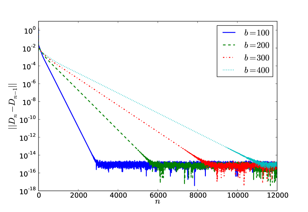
Figure 7.1. Convergence of the Level-Shifting algorithm. The convergence is linear until machine precision. The horizontal spacing of the curves reveals the asymptotic relationship $\nu\propto\frac{1}{b}$. The system considered is the carbon atom ($N=Z=6$), under the RHF formalism, using the 3-21G gaussian basis functions.

Next, we compared the efficiency of the Roothaan algorithm and of the gradient algorithm, in the case where the Roothaan algorithm converges. Our analysis leads to the estimate $\nu=\frac{\gamma}{8{\kappa^{\prime}}^{2}\mathinner{\!\left\lVert F\right\rVert}_{\text{op}}^{2}}$ for the Roothaan algorithm, and $\nu=\frac{1}{4\kappa^{2}\alpha}$ for the gradient algorithm with stepsize $t=\frac{1}{\alpha}$.

It is immediate to see that, up to a constant multiplicative factor, $\kappa^{\prime}>\kappa$, $\gamma\leq\mathinner{\!\left\lVert F\right\rVert}_{\text{op}}$ and for the cases of interest $\alpha\approx\mathinner{\!\left\lVert F\right\rVert}_{\text{op}}$, so from our estimates we would expect the gradient algorithm to be faster than the Roothaan algorithm. However, in our tests the Roothaan algorithm was considerably faster than the gradient algorithm (see Figure 7.2). This conclusion holds even when the stepsize is adjusted at each iteration with a line search.

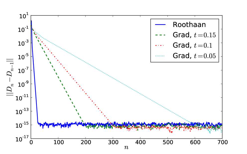
Figure 7.2. Comparison of Roothaan and gradient algorithm. The system considered is the carbon atom ($N=Z=6$), under the RHF formalism, using the 3-21G gaussian basis functions.

The reason that the Roothaan algorithm performs better than expected is that the inequality

$$\mathinner{\!\left\lVert[D_{k+2}-D_{k},F(D_{k+1})]\right\rVert}\leq 2\mathinner{\!\left\lVert F(D_{k+1})\right\rVert}\mathinner{\!\left\lVert D_{k+2}-D_{k}\right\rVert}$$

is very far from optimal. Whether an improved bound (in particular, one that does not depend on the dimension) can be derived is an interesting open question.

The outcome of these tests seems to be that the gradient algorithm is slower. It might prove to be faster in situations where the gap is small, or whenever $\kappa^{\prime}$ is much larger than $\kappa$. We have been unable to find concrete examples of such cases.

8. Conclusion, perspectives

In this paper, we introduced an algorithm based on the idea of gradient descent. By using the analyticity of the objective function and of the constraint manifold, we were able to derive a Łojasiewicz inequality, and use that to prove the convergence of the gradient method, under the assumption of a small enough stepsize. Next, expanding on the analysis of [5], we extended the Łojasiewicz inequality to a Lyapunov function for the Roothaan algorithm. By linking the gradient of this Lyapunov function to the difference in the iterates of the algorithm, we proved convergence (or oscillation), an improvement over previous results which only prove a weaker version of this. In this framework, the Level-Shifting algorithm can be seen as a simple modification of the Roothaan algorithm, and as such can be treated by the same methods. In each case, we were also able to derive explicit bounds on the convergence rates.

The strength of the Łojasiewicz inequality is that no higher-order hypothesis are needed for its use. As a consequence, the rates of convergence we obtain weaken considerably if the algorithm converges to a degenerate critical point. A more precise study of the local structure of critical points is necessary to understand why the algorithms usually exhibit geometric convergence. This is related to the problem of local uniqueness and is likely to be hard (and, indeed, to our knowledge has not been tackled yet).

Even though our results hide the complexity of the local structure in the constants of the Łojasiewicz inequality, they still provide insight as to the influence of the basis on the speed of convergence, and can be used to compare algorithms. All of our results use crucially the hypothesis of a finite-dimensional Galerkin space. For the gradient algorithm, we need it to ensure the existence of a stepsize that decreases the energy. This is analogous to a CFL condition for the discretization of the equation $\mathinner{\frac{\operatorname{d\!}{}D}{\operatorname{d\!}{t}}}=-[D,[D,F_{D}]]$, and can only be lifted with a more implicit discretization of this equation. For the Roothaan and Level-Shifting algorithms, we use the finite dimension hypothesis to bound $F(D)$. As noted in Section 7, the inequality is not sharp, so it could be that the infinite-dimensional version of the Roothaan and Level-Shifting algorithms still converge. More research is needed to examine this.

The gradient algorithm we examined only converges towards a stationary point of the energy, that may not be a local minimizer, or even an Aufbau solution. However, it will generically converge towards a local minimizer, unlike the Level-Shifting algorithm with large $b$. Therefore, it is the most robust of the algorithms considered. Although it was found to be slower than other algorithms on the numerical tests we performed, it has the advantage that its convergence rate does not depend on the gap $\lambda_{N+1}-\lambda_{N}$, and might therefore prove useful in extreme situations.

An algorithm that could achieve the speed of the fixed-point algorithms with the robustness granted by the energy monotonicity seems to be the ODA algorithm of Cancès and Le Bris[5], along with variants such as EDIIS, or combinations of EDIIS and DIIS algorithms[12]. We were not able to examine these algorithms in this paper. At first glance, the ODA algorithm should fit into our framework (indeed, the ODA algorithm was built to satisfy an energy decrease inequality similar to (3.7)). However, it works in a relaxed parameter space $\widetilde{P}$, and using the commutator to control the differences of iterates as we did only makes sense on $\mathcal{P}$. Therefore, other arguments have to be used.

A variant on the gradient algorithm used here is to modify the local geometry of the manifold $\mathcal{P}$ by using a different inner product, leading to a variety of methods, including conjugate gradient algorithms[8]. These methods fit into our framework, as long as one can prove that they are “gradient-like”, in the sense that one can control the gradient by the difference $D_{k+1}-D_{k}$. However, precise estimates of convergence rates might be hard to obtain.

Also missing from the present contribution is the study of other commonly used algorithms, such as DIIS[17], and variants of (quasi)-Newton algorithms[2, 11]. DIIS numerically exhibits a complicated behavior that is probably hard to explain analytically, and the (quasi)-Newton algorithms require a study of the second-order structure of the critical points, which we are unable to do.

9. Acknowledgments

The author would like to thank Eric Séré for his extensive help, Guillaume Legendre for the code used in the numerical simulations and Julien Salomon for introducing him to the Łojasiewicz inequality. He also thanks the anonymous referees for many constructive remarks.

References

• [1] F. Alouges and C. Audouze. Preconditioned gradient flows for nonlinear eigenvalue problems and application to the Hartree-Fock functional. Numerical Methods for Partial Differential Equations, 25(2):380–400, 2009.
• [2] G.B. Bacskay. A quadratically convergent Hartree–Fock (QC-SCF) method. Application to closed shell systems. Chemical Physics, 61(3):385–404, 1981.
• [3] E. Cancès, M. Defranceschi, W. Kutzelnigg, C. Le Bris, and Y. Maday. Computational quantum chemistry: a primer. Handbook of numerical analysis, 10:3–270, 2003.
• [4] E. Cancès and C. Le Bris. Can we outperform the DIIS approach for electronic structure calculations? International Journal of Quantum Chemistry, 79(2):82–90, 2000.
• [5] E. Cancès and C. Le Bris. On the convergence of SCF algorithms for the Hartree-Fock equations. Mathematical Modelling and Numerical Analysis, 34(4):749–774, 2000.
• [6] E. Cancès and K. Pernal. Projected gradient algorithms for Hartree-Fock and density matrix functional theory calculations. The Journal of chemical physics, 128:134108, 2008.
• [7] E. Cancès. SCF algorithms for Hartree-Fock electronic calculations. In M. Defranceschi and C. Le Bris, editors, Mathematical models and methods for ab initio quantum chemistry, Lecture Notes in Chemistry, volume 74. Springer, 2000.
• [8] A. Edelman, T.A. Arias, and S.T. Smith. The Geometry of Algorithms with Orthogonality Constraints. SIAM Journal on Matrix Analysis and Applications, 20:303, 1998.
• [9] J.B. Francisco, J.M. Martínez, and L. Martínez. Globally convergent trust-region methods for self-consistent field electronic structure calculations. The Journal of chemical physics, 121:10863, 2004.
• [10] A. Haraux, M.A. Jendoubi, and O. Kavian. Rate of decay to equilibrium in some semilinear parabolic equations. Journal of Evolution equations, 3(3):463–484, 2003.
• [11] S. Høst, J. Olsen, B. Jansík, L. Thøgersen, P. Jørgensen, and T. Helgaker. The augmented Roothaan–Hall method for optimizing Hartree–Fock and Kohn–Sham density matrices. The Journal of chemical physics, 129:124106, 2008.
• [12] K.N. Kudin, G.E. Scuseria, and E. Cancès. A black-box self-consistent field convergence algorithm: One step closer. The Journal of chemical physics, 116:8255, 2002.
• [13] E.H. Lieb and B. Simon. The Hartree-Fock theory for Coulomb systems. Communications in Mathematical Physics, 53(3):185–194, 1977.
• [14] P.L. Lions. Solutions of Hartree-Fock equations for Coulomb systems. Communications in Mathematical Physics, 109(1):33–97, 1987.
• [15] S. Łojasiewicz. Ensembles semi-analytiques. Institut des Hautes Etudes Scientifiques, 1965.
• [16] R. McWeeny. The density matrix in self-consistent field theory. I. Iterative construction of the density matrix. Proceedings of the Royal Society of London. Series A. Mathematical and Physical Sciences, 235(1203):496, 1956.
• [17] P. Pulay. Improved SCF convergence acceleration. Journal of Computational Chemistry, 3(4):556–560, 1982.
• [18] J. Salomon. Convergence of the time-discretized monotonic schemes. ESAIM: Mathematical Modelling and Numerical Analysis, 41(01):77–93, 2007.
• [19] V.R. Saunders and I.H. Hillier. A “Level–Shifting” method for converging closed shell Hartree–Fock wave functions. International Journal of Quantum Chemistry, 7(4):699–705, 1973.
• [20] R.B. Sidje. Expokit: a software package for computing matrix exponentials. ACM Transactions on Mathematical Software (TOMS), 24(1):130–156, 1998.