Sudden switch of generalized Lieb-Robinson velocity in a transverse field Ising spin chain

Abstract

The Lieb-Robinson theorem states that the speed at which the correlations between two distant nodes in a spin network can be built through local interactions has an upper bound, which is called the Lieb-Robinson velocity. Our central aim is to demonstrate how to observe the generalized Lieb-Robinson velocity in an Ising spin chain with a strong transverse field. Here the generalized Lieb-Robinson velocity is defined as the correlation propagation speed from a given initial non-correlated state, which is upper bounded by the Lieb-Robinson velocity. We adopt and compare four correlation measures for characterizing different types of correlations, which include correlation function, mutual information, quantum discord, and entanglement of formation. All the information-theoretical correlation measures demonstrate the existence of the generalized Lieb-Robinson velocity. In particular, we find that there is a sudden switch of the generalized Lieb-Robinson speed with the increasing of the number of spin.

I introduction

The correlations in a quantum many-body system make its physical properties can not be regarded as the simple sum of the properties of the composite subsystems. Recent studies of correlations in quantum information science show that correlations can be used as indispensable resources in completing some computing and information tasks HHHH81 . Thus the correlations play a key role both in quantum many-body physics and in quantum information science.

The correlations in a many-body system can be classified into different types according to different standards, where the two-party correlation is relatively well understood and widely used in practical problems. The two-party correlations in a many-body quantum state are measured by correlation functions associated with physical observables in traditional physics, while they are measured by the mutual entropy in quantum information. The two-party correlations can be further classified into quantum two-party correlations and classical two-party correlations, and entanglement is a specific type of quantum correlations, which is extensively investigated in quantum information science. The measures of different types of corrrelations are proposed in literature. The widely used entanglement measure is the entanglement of formation (EoF) HW97 ; Wooters98 , and quantum discord (QD) OZ01 ; HV01 ; DSC08 is used to characterize the quantum correlations.

Recently, many investigations have been made in understanding the dynamical creation and evolution of correlations between the nearest-neighbor particle pairs and between two distant particles which are not connected by direct interactions in the spin chain model, for example, $XX$, $XY$, and Ising model systems Cirac08 ; Sokolovsky08 ; Sen09 ; NWu10 ; Kais11 . As we know, if two particles directly interact with each other, then the correlations between these two particles can be built dynamically from an initial state without correlations. However, if two distant particles in a quantum network indirectly interact through local interactions, how fast will the correlations between these two distant particles be dynamically generated? The Lieb-Robinson theorem LR72 ; MBHastingsB04 ; MBHastingsL04 ; BHV97 ; NS06 ; NYS124 gives an intriguing answer to this question: The speed of the correlations between two distant particles has an upper bound, which is called the Lieb-Robinson velocity. In other words, the correlations outside the light cone defined by the Lieb-Robinson velocity can be neglected. Recently, the Lieb-Robinson theorem has received renewed interest and has been applied to the condensed matter theory and quantum information theory BO99 ; EO97 ; MMGC82 ; Poulin ; SH81 . For example, it can be used to derive a general relation on the two-party correlations in the many-body ground states.

As an upper bound on the speed of correlation generation, can the Lieb-Robinson velocity be observed in a concrete quantum network? As far as we know, there is no related experimental report so far. In fact, we can obtain the Lieb-Robinson velocity through finding the maximum generalized Lieb-Robinson velocity in all kinds of conditions. Here the generalized Lieb-Robinson velocity is defined as the correlation propagation speed from a given initial non-correlated state, which is upper bounded by the Lieb-Robinson velocity. In this paper, our central aim is to demonstrate how to observe the generalized Lieb-Robinson velocity in an Ising spin chain with a strong transverse field. To solve this problem, we first need to choose a model whose dynamics relatively easy to simulate. Then we need the measures to characterize different types of correlations. Finally, we need to give a criterion to judge whether the correlations between two distant particles appears. It should be pointed out that the generalized Lieb-Robinson velocity we study in this article is not the upper bound of speed but the concrete propagation velocity of correlation. In this article, we choose the transverse field Ising chain as the basic model, which is exactly solvable for eigen problems. We consider the measures of different types of correlations, including correlation functions, mutual entropy, EoF, and QD. Thus we can investigate whether the generalized Lieb-Robinson velocity depends on the correlation measures. The criterion for correlation appearance is to set the correlation measure to a value numerically so small such that the correlation appearance time is almost fixed.

In our article, we find that the generalized Lieb-Robinson velocity can be obtained by analyzing a correlation measure. Almost all types of correlation measures can demonstrate the generalized Lieb-Robinson velocity in their dynamics. In particular, we find a sudden switch of the generalized Lieb-Robinson velocities with the increasing of the spin number. This paper is organized as follows. In Sec. II, we will briefly introduce the physical model and the solution of the dynamics for the reduced two-particle state. In Sec. III, we will study and compare the dynamics of different kinds of correlations, and show the relation between the evolution of correlations and the length of the spin chain. In Sec. IV, we will study the buildup of correlations. Finally, we will give a brief summary.

II Model, approximation and solution

We will consider a transverse field Ising spin chain (TFIC) with free ends, whose Hamiltonian can be written as

$$H=-J\sum_{i=1}^{N-1}\sigma_{i}^{z}\sigma_{i+1}^{z}-B\sum_{i=1}^{N}\sigma_{i}^{x},$$ (1)

where $J$ is the coupling constant, $B$ is the strength of the transverse filed, $N$ is the total number of spin, and $\sigma_{i}^{\alpha}\left(\alpha=x,y,z\right)$ are the Pauli operators acting on the $i$-th spin of the chain.

To investigate the dynamical creation of correlations along a TFIC, we consider the following physical process. First, let the system stay in the ground state of the system. Then flip the first spin. Our aim is to observe how the correlations between the first spin and the last spin will be created dynamically. The physical setting is demonstrated in Fig. 1.

Figure 1: Dynamical generation of correlations between the first spin and the last spin in the spin chain ($N=7$).

II.1 Rotating-wave approximation for TFIC in a strong magnetic field

In the weak coupling region ($J\ll B$), the Hamiltonian (1) can be rephrased in the following more convenient form

$$H = -J\sum_{i=1}^{N-1}\left(\sigma_{i}^{-+}\sigma_{i+1}^{+-}+\sigma_{i}^{+-}\sigma_{i+1}^{-+}+\sigma_{i}^{-+}\sigma_{i+1}^{-+}\right.$$ (2)

$$\left.+\sigma_{i}^{+-}\sigma_{i+1}^{+-}\right)-B\sum_{i=1}^{N}\sigma_{i}^{x},$$

where $\left|\pm\right\rangle_{i}$ are the two eigenvectors of $\sigma_{i}^{x}$, and $\sigma_{i}^{\mu\nu}$=$\left|\mu\right\rangle_{i}\left\langle\nu\right|_{i}$ with $\mu,\nu\in\{+,-\}$. Under the rotating-wave approximation (RWA) scully , the Hamiltonian becomes

$$H_{\text{RWA}}=-J\sum_{i=1}^{N-1}\left(\sigma_{i}^{-+}\sigma_{i+1}^{+-}+\sigma_{i}^{+-}\sigma_{i+1}^{-+}\right)-B\sum_{i=1}^{N}\sigma_{i}^{x}.$$ (3)

The Hamiltonian $H_{\text{RWA}}$ is unitarily equivalent to the $XY$ spin model. Notice that in the above Hamiltonian (3), the $x$-component of the total spin $\sigma_{T}^{x}=\sum_{i=1}^{N}\sigma_{i}^{x}$ is conserved. In other words, an invariant subspace of the Hamiltonian can be characterized by a given eigenvalue of $\sigma_{T}^{x}$, and the dynamics of the system can be studied independently in these invariant subspaces.

Before investigating further the dynamics of the system, we directly check the validity of RWA for the Hamiltonian by numerically comparing the eigenvalues and the eigenvectors between the Hamiltonian without RWA (1) and the one with RWA (3). The numerical results for $N=3$ are demonstrated in Fig. 2. As expected, we find that RWA is an excellent approximation as long as $B\gg J.$

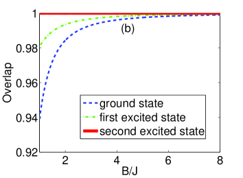
Figure 2: (Color online) (a) The energy spectrum ($N=3$) as a function of $B/J$. Dashed lines: the result in RWA; Solid lines: the result without RWA. (b) The overlap between the wave function obtained with RWA and without RWA as a function of $B/J$. Dashed line: the overlap of ground states; Dotted-dashed line: the overlap of the first exctied states; Sloid line: the overlap of the second excited states.

II.2 Quantum state evolution under RWA

In this section, we will obtain the analytical results on the quantum state evolution of the system under RWA.

In the ground state of the Hamiltonian $H_{\text{RWA}}$, all the spins point along the positive direction of $x$ axis. While flipping the first spin, we get the initial state $|\psi(0)\rangle=|-++\cdots+\rangle$. Because $\sigma_{T}^{x}|\psi(0)\rangle=(N-2)|\psi(0)\rangle$ and $[\sigma_{T}^{x},H_{\text{RWA}}]=0$, the quantum state will evolve with time in the eigen space of $\sigma_{T}^{x}$ with eigenvalue $N-2$. All the eigenvectors of the subspace can be denoted as $|m\rangle=\prod_{i=1}^{m-1}|+\rangle_{i}|-\rangle_{m}\prod_{j=m+1}^{N}|+\rangle_{j}$ for $m\in\{1,2,\cdots,N\}$. Using these new notations, the initial state $|\psi(0)\rangle=|1\rangle$, and the Hamiltonian in this subspace

$$H=-(N-2)B-J\left(\begin{array}[]{ccccc}0&1&0&\cdots&0\\ 1&0&1&\cdots&0\\ 0&1&0&\cdots&0\\ \vdots&\vdots&\vdots&\ddots&1\\ 0&0&0&1&0\end{array}\right).$$ (4)

The Hamiltonian $H_{\text{RWA}}$ has eigenstates

$$\left|\psi_{k}\right\rangle=\sqrt{\frac{2}{N+1}}\sum_{n=1}^{N}\sin\left(\frac{\pi kn}{N+1}\right)\left|n\right\rangle,$$ (5)

with eigenvalues

$$E_{k}=-(N-2)B+2J\cos\frac{k\pi}{N+1},$$ (6)

for $k=1,2,\cdots,N$.

The quantum state of the system at time $t$ is given by

$$\left|\Psi(t)\right\rangle = \sum_{n=1}^{N}A_{n}\left|n\right\rangle,$$ (7)

where

$$A_{n}=\frac{2}{N+1}\sum_{k=1}^{N}e^{-iE_{k}t}\sin\left(\frac{\pi k}{N+1}\right)\sin\left(\frac{\pi kn}{N+1}\right).$$ (8)

Since we will consider the correlations between the first spin and the last spin, we only need the reduced density matrix of these two spins, which is given by

$$\rho_{1N}=\left(\begin{array}[]{cccc}0&0&0&0\\ 0&\left|A_{1}\right|^{2}&A_{1}^{\ast}A_{N}&0\\ 0&A_{1}A_{N}^{\ast}&\left|A_{N}\right|^{2}&0\\ 0&0&0&1-\left|A_{1}\right|^{2}-\left|A_{N}\right|^{2}\end{array}\right).$$ (9)

The above formula implies that only $A_{1}$ and $A_{N}$ are needed to be calculated for our purpose, which reduces a large amount of computation.

III dynamics of different types of correlations

To study the correlations between the first spin and the last spin, we adopt both traditional method and information method to characterize the degrees of correlations. In this section, we will numerically study the dynamical evolution of different measures of correlations between the first spin and the last spin. The correlation measures we adopt include the correlation functions, the mutual information, quantum discord, and the entanglement of formation. We aim to find out the relation between the evolution of correlations and the length of spin chain.

III.1 Traditional method: Correlation function

Correlation function (CF) is a traditional tool in describing the correlation effects in a many-body system. For a two-qubit system, the CFs are defined by DZ10

$$C_{F}\left(\sigma_{1}^{\alpha},\sigma_{N}^{\beta}\right)=\mathrm{Tr}\left(\rho_{1N}\sigma_{1}^{\alpha}\sigma_{N}^{\beta}\right)-\mathrm{Tr}\left(\rho_{1}\sigma_{1}^{\alpha}\right)\mathrm{Tr}\left(\rho_{N}\sigma_{N}^{\beta}\right),$$ (10)

where $\alpha,\beta\in\left\{x,y,z\right\}$, and $\rho_{1}$ and $\rho_{N}$ are the reduced density matrices of the bipartite quantum state $\rho_{1N}.$ Inserting Eq. (9) into Eq. (10), we have

$$C_{F}\left(\sigma_{1}^{z},\sigma_{N}^{z}\right) = -4\left|A_{1}\right|^{2}\left|A_{N}\right|^{2},$$ (11)

$$C_{F}\left(\sigma_{1}^{x},\sigma_{N}^{x}\right) = A_{1}A_{N}^{\ast}+A_{1}^{\ast}A_{N}.$$ (12)

Here we find that $C_{F}\left(\sigma_{1}^{x},\sigma_{N}^{x}\right)=0$ when $N$ is even. This result can be proved as follows. We have the relation

$$C_{F}\left(\sigma_{1}^{x},\sigma_{N}^{x}\right) = A_{1}A_{N}^{\ast}+A_{1}^{\ast}A_{N}$$ (13)

$$= \frac{8}{(N+1)^{2}}\sum_{k,m=1}^{N}\cos\left[\left(E_{k}-E_{m}\right)t\right]\left(-1\right)^{m+1}\sin^{2}\left(\frac{k\pi}{N+1}\right)\sin^{2}\left(\frac{m\pi}{N+1}\right)$$

$$= \frac{8}{(N+1)^{2}}\sum_{k,m=1}^{N}\cos\left[2J\left(\cos\frac{m\pi}{N+1}-\cos\frac{k\pi}{N+1}\right)t\right]$$

$$\times\left(-1\right)^{m+1}\sin^{2}\left(\frac{k\pi}{N+1}\right)\sin^{2}\left(\frac{m\pi}{N+1}\right)$$

$$= \frac{8}{(N+1)^{2}}\sum_{l=1}^{N}\sum_{k=1}^{N}\cos\left[2J\left(\cos\frac{(N+1-l)\pi}{N+1}-\cos\frac{(N+1-k)\pi}{N+1}\right)t\right]$$

$$\times\left(-1\right)^{(N+1-l)+1}\sin^{2}\left(\frac{(N+1-k)\pi}{N+1}\right)\sin^{2}\left(\frac{(N+1-l)\pi}{N+1}\right)$$

$$\text{}= (-1)^{N+1}C_{F}(\sigma_{1}^{x},\sigma_{N}^{x}).$$

When $N$ is even, we have $C_{F}(\sigma_{1}^{x},\sigma_{N}^{x})=-C_{F}(\sigma_{1}^{x},\sigma_{N}^{x})$, which implies that $C_{F}(\sigma_{1}^{x},\sigma_{N}^{x})=0$.

It is worth pointing out that $C_{F}(\sigma_{1}^{z},\sigma_{N}^{z})\neq 0$ whether $N$ is odd or even. These different correlation behaviors between $C_{F}(\sigma_{1}^{x},\sigma_{N}^{x})$ and $C_{F}(\sigma_{1}^{z},\sigma_{N}^{z})$ shows that the correlations measured by correlation functions depend on which correlation function we choose. In the viewpoint of quantum information, correlation in a two-partite quantum state is a property of the state, and the characterization of the correlation does not depend on what measurements we obtain the correlation. This information viewpoint will be detailedly discussed in the next section.

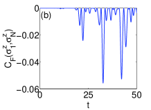
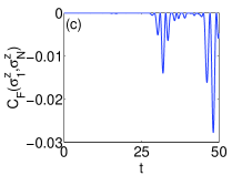
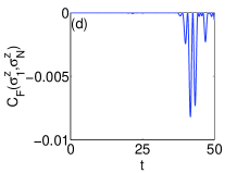
Figure 3: Dynamics of correlation function $C_{F}\left(\sigma_{1}^{z},\sigma_{N}^{z}\right)$ of the spin chain with different lengths: (a) $N=10$, (b) $N=20$, (c) $N=30$, (d) $N=40$.

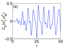
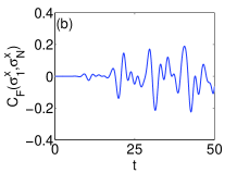
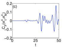
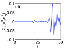
Figure 4: Dynamics of correlation function $C_{F}\left(\sigma_{1}^{x},\sigma_{N}^{x}\right)$ of the spin chain with different lengths: (a) $N=9$, (b) $N=19$, (c) $N=29$, (d) $N=39$.

The numerical results about the dynamical evolution of the two CFs, $C_{F}\left(\sigma_{1}^{z},\sigma_{N}^{z}\right)$ and $C_{F}\left(\sigma_{1}^{x},\sigma_{N}^{x}\right)$, of the spin chain with different lengths are shown in Fig. 3 and Fig. 4. From the two figures, we can observe that the creation of correlations between the first spin and the last spin, which have no direct interactions, is not instantaneous but requires the formation time, and the formation time is directly proportional to the length of spin chain. In other words, the longer the distance between the first spin and the last spin is, the more time the appearance of their correlation needs.

III.2 Information method: Mutual information, quantum discord, entanglement of formation

In quantum information science, the characterization of correlations in a bipartite quantum state is relatively well understood. The degree of the total correlation in a bipartite quantum state is measured by the mutual entropy. The total correlation can be classified into classical correlation and quantum discord OZ01 ; HV01 . Quantum entanglement is a special type of quantum discord. The classification of correlations is demonstrated in Fig. 5.

Figure 5: Demonstration of classification of the total correlation meausred by mutual entropy. Classical correlation, quantum discord, quantum entanglement are abbraviated as CC, QD, and QE respectively.

The total correlation between two subsystems A and B are quantified by the mutual information (MI)

$$\mathcal{I}(\rho^{AB})=S(\rho^{A})+S(\rho^{B})-S(\rho^{AB}),$$ (14)

where $S(\rho)\equiv-\mathrm{Tr}(\rho\log_{2}\rho)$ is the von Neumann entropy. To define the classical correlation contained in the state $\rho^{(AB)}$, we consider the following process. B performs a projective measurement $\{\Pi_{j}\}$ on the subsystem B, and will get a state

$$\rho_{k}^{A}=\frac{1}{p_{k}}\mathrm{Tr_{B}}\left(I\otimes\Pi_{k}\rho^{AB}I\otimes\Pi_{k}\right),$$ (15)

with the corresponding probability $p_{k}=\mathrm{Tr_{AB}}\left(I\otimes\Pi_{k}\rho^{AB}I\otimes\Pi_{k}\right)$. By performing a measurement on subsystem A, A wants to give the information on which measurement result got by B. The upper bound of the information is the Holevo bound

$$\chi(\rho^{AB}|\{\Pi_{k}\})=S(\rho^{A})-p_{k}S(\rho_{k}^{A}).$$ (16)

Then a measure of classical correlation (CC) in the state $\rho^{(AB)}$ is defined by

$$\mathcal{J}(\rho^{AB})=\max_{\{\Pi_{k}\}}\chi(\rho^{AB}|\{\Pi_{k}\}).$$ (17)

Once CC is obtained, the QD is obtained by subtracting CC from the MI

$$\mathcal{D}(\rho^{AB})=\mathcal{I}(\rho^{AB})-\mathcal{J}(\rho^{AB}).$$ (18)

Quantum entanglement is a special type of quantum discord, which is widely investigated in quantum information. One of the most useful measures of entanglement is entanglement of formation HW97 ; Wooters98 , which is defined by

$$\mathcal{E}(\rho^{(AB)})=\frac{1}{2}\min_{\{p_{i},|\psi_{i}\rangle\}}p_{i}\mathcal{I}(|\psi_{i}^{(AB)}\rangle),$$ (19)

where $\rho^{(AB)}=\sum_{i}p_{i}|\psi_{i}^{(AB)}\rangle\langle\psi_{i}^{(AB)}|$.

For a two-qubit system, all the above correlation measures can be obtained analytically or numerically. For example, in our case, the mutual information is

$$\mathcal{I}(1,N) = \left|A_{N}\right|^{2}\log_{2}\left[\frac{\left(1-\left|A_{N}\right|^{2}\right)\left(\left|A_{1}\right|^{2}+\left|A_{N}\right|^{2}\right)}{\left|A_{N}\right|^{2}\left(1-\left|A_{1}\right|^{2}-\left|A_{N}\right|^{2}\right)}\right]$$ (20)

$$+\left|A_{1}\right|^{2}\log_{2}\left[\frac{\left(1-\left|A_{1}\right|^{2}\right)\left(\left|A_{1}\right|^{2}+\left|A_{N}\right|^{2}\right)}{\left|A_{1}\right|^{2}\left(1-\left|A_{1}\right|^{2}-\left|A_{N}\right|^{2}\right)}\right]$$

$$+\log_{2}\left[\frac{1-\left|A_{1}\right|^{2}-\left|A_{N}\right|^{2}}{\left(1-\left|A_{1}\right|^{2}\right)\left(1-\left|A_{N}\right|^{2}\right)}\right],$$

which is shown in Fig. 6. Following the method introduced in Ref. ali ; luo1 , we can numerically obtain the dynamical evolution of QD as shown in Fig. 7. In order to compare the dynamical evolution between MI(QD) and EoF, we also plot the dynamical evolution of EoF as shown in Fig. 8.

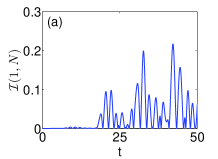
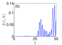
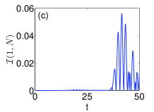
Figure 6: Dynamics of MI of the spin chain with different lengths: (a) $N=20$, (b) $N=30$, (c) $N=40$, (d) $N=500$.

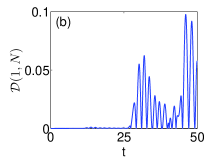
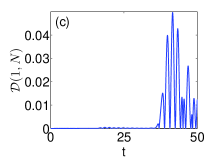
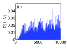
Figure 7: Dynamics of QD of the spin chain with different lengths: (a) $N=20$, (b) $N=30$, (c) $N=40$, (d) $N=500$.

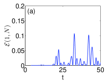
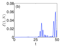
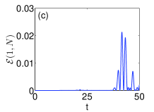
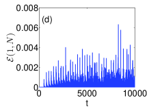
Figure 8: Dynamics of EoF of the spin chain with different lengths: (a) $N=20$, (b) $N=30$, (c) $N=40$, (d) $N=500$.

In Fig. 6, Fig. 7, and Fig. 8, we plot four cases in each figure, that is, $N=20$, $N=30$, $N=40$, and $N=500$, in order to find the relation between the dynamical evolution and the length of spin chain. From these three figures, we observe that the dynamical evolutions of MI, QD and EoF are similar with CFs, that is, the creation of MI, QD and EoF between the first spin and the last spin is not instantaneous but requires the formation time, and the longer the spin chain is, the more time to create correlations takes. In addition, the maximum amplitudes that the MI, QD and EoF can reach all become smaller with the increase of the length of spin chain. However, the degrees of amplitude reduction are not same. For example, we consider $N=500,$ from Fig.6, Fig.7, and Fig.8, we can see that the maximum amplitudes of MI and QD are about $4\times 10^{-2}$, while the maximal amplitude of EoF is only about $6\times 10^{-3},$ which implies that MI and QD are more robust to the length increase of the spin chain than EoF.

IV Start-up time with different chain lengths

In the above section we have shown that the time needed to create correlations between the first spin and the last spin increases with the increase of the spin chain length. However, we still do not know how fast correlations can be created between the first spin and the last spin in our concrete model, though there is an obvious and correct answer: No faster than the Lieb-Robinson speed. In this section, we will numerically study the relation between the start-up time of correlations for different correlation measures and the length of spin chain. We aim to find out the propagation speed of correlations and investigate whether the propagation speed depends on the correlation measures.

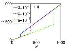
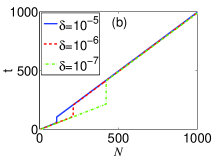
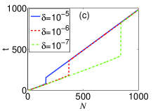
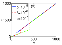
Figure 9: (Color online) Start-up time of (a) MI, (b) EoF, (c) QD, and (d) CC as a function of $N$ with different criteria. The criteria of solid line, dashed line, and dotted-dashed line are $\delta=10^{-4},$ $\delta=10^{-5},$ and $\delta=10^{-6}$, respectively.

Fig. 9 shows the start-up time of MI, QD, EoF, and CC as a function of $N$, the length of spin chain, where $N$ is an integer we choose from $2$ to $1000$. Here we define the criterion for correlation appearance, which can be used to judge whether the correlations have been created or not at a given time. In every subfigure of Fig. 9, we plot three curves. Different curves have different criteria of start-up $\delta$, that is, the criteria of solid line, dashed line, and dotted-dashed line are $\delta=10^{-4},$ $\delta=10^{-5},$ and $\delta=10^{-6}$, respectively. From Fig. 9, we observe that the start-up time as a function of the spin chain length has two segments, and there is a sudden switch point, which moves rightwards with the decrease of the criterion. From Fig. 6, Fig. 7 ,and Fig. 8, we can see that there are a series of obvious peaks in the figures. In fact, the first segment in Fig. 9 appears since the first peak reaches the criterion, and the second segment appears since the second peak reaches the criterion. Thus we plot the first peak value of MI as a function of the spin chain length as shown in Fig. 10. We find the relation between $\log\mathcal{I}$ and $\log N$ is linear, that is

$$\mathcal{I}=N^{\alpha}e^{\beta},$$ (21)

where $\alpha=-2.8529$ and $\beta=3.0981$. We also plot the second peak value of MI as a function of the spin chain length as shown in Fig. 10, the relation between $\log\mathcal{I}$ and $\log N$ is also linear, but $\alpha=-0.9257$ and $\beta=0.5725$. So the first peak will disappear sooner than the second peak with the increase of $N$. This implies that the first peak becomes lower than the criterion with the increase of $N$, but the second peak is still higher than the criterion. This is the reason for the appearance of switch point in Fig. 9.

Figure 10: $\log\mathcal{I}$ is linearly proportional to $\log N$ for (a) the first peak value, (b) the second peak value.

Lastly, in order to investigate whether the propagation speed depends on the correlation measures, we plot them in the same figure with the criterion $\delta=10^{-6}$ as shown in Fig. 11 to compare the start-up times of MI, QD, CC and EoF. We find that the propagation velocity does not depend on the correlation measures, but the sudden switch point depends on the correlation measures.

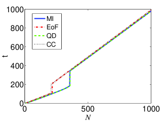
Figure 11: (Color online) Comparison of start-up times of MI, QD, CC and EoF with the criterion $\delta=10^{-6}$.

In the above numerical results, the correlation start-up time is linearly proportional to the length of the spin chain, which implies the existence of the generalized Lieb-Robinson velocity. The sudden switch of the generalized Lieb-Robinson velocities implies that different types of correlations may have different generalized Lieb-Robinson velocities. In the present model, the amplitudes of these two types of correlations decreases exponentially with the length of the spin chain, and these two types of correlations are characterized by different exponential indexes. It is these different characteristics of correlations that lead to the sudden switch of the Lieb-Robinson velocities.

V Discussion and Conclusion

We have numerically investigated the problem on the generalized Lieb-Robinson velocities in TFIC. We show that the generalized Lieb-Robinson velocity can be observed by the dynamics of the correlations between the first spin and the last spin. A sudden switch of the generalized Lieb-Robinson velocities appears in TFIC. Here a main open problem is whether the phenomena in TFIC are model independent. However, the method we adopt for TFIC uses the analytical results, which is not available for a general spin model. In addition, as far as we know, the algorithms for quantum dynamics are not powerful enough to simulating for a sufficient long time with a long spin chain. In this direction, we study another related mode, the isotropic Heisenberg chain.

The start-up time of CF of isotropic Heisenberg chain with uniform coupling as a function of the chain length $N$ is demonstrated in Fig. 12. We find that the phenomena on the generalized Lieb-Robinson velocity have the same characteristic in the isotropic Heisenberg chain.

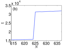
Figure 12: Start-up time of CF of the Heisenberg chain with uniform coupling as a function of $N$: (a) from $N=2$ to $N=200$, (b) from $N=614$ to $N=637$.

In conclusion, we have numerically investigated the generalized Lieb-Robinson velocity in an Ising spin chain with a strong transverse field through studying the dynamical evolution of correlations. The generalized Lieb-Robinson velocities are demonstrated in different types of correlation measures, which include correlation function, mutual information, quantum discord, and entanglement of formation. We find that one of the correlation functions shows a special behavior depending on the parity of the spin number. In particular, we find that there is a switch in the generalized Leb-Robinson velocities, which implies that different types of correlations may show different generalized Lieb-Robinson velocities.

- (1) R. Horodecki, P. Horodecki, M. Horodecki, and K. Horodecki, Rev. Mod. Phys. 81, 865 (2009).
- (2) S. Hill and W. K. Wootters, Phys. Rev. Lett. 78, 5022 (1997).
- (3) W. K. Wootters, Phys. Rev. Lett. 80, 2245 (1998).
- (4) H. Ollivier and W. H. Zurek, Phys. Rev. Lett. 88, 017901 (2001).
- (5) L. Henderson and V. Vedral, J. Phys. A: Math. Gen. 34, 6899 (2001).
- (6) A. Datta, A. Shaji, and C. M. Caves, Phys. Rev. Lett. 100, 050502 (2008).
- (7) T. S. Cubitt and J. I. Cirac, Phys. Rev. Lett. 100, 180406 (2008).
- (8) G. B. Furman, V. M. Meerovich, and V. L. Sokolovsky, Phys. Rev. A 77, 062330 (2008).
- (9) K. Sengupta and D. Sen, Phys. Rev. A 80, 032304 (2009).
- (10) Z. Chang and N. Wu, Phys. Rev. A 81, 022312 (2010).
- (11) B. Alkurtass, G. Sadiek, and S. Kais, Phys. Rev. A 84, 022314 (2011).
- (12) E. H. Lieb and D.W. Robinson, Commun. Math. Phys. 28, 251 (1972).
- (13) M. B. Hastings, Phys. Rev. B 69, 104431 (2004).
- (14) M. B. Hastings, Phys. Rev. Lett. 93, 140402 (2004).
- (15) S. Bravyi, M.B. Hastings, and F. Verstraete, Phys. Rev. Lett. 97, 050401 (2006).
- (16) B. Nachtergaele and R. Sims, Commun. Math. Phys. 265, 119 (2006).
- (17) B. Nachtergaele, Y. Ogata, and R. Sims, J. Stat. Phys. 124, 1 (2006) .
- (18) J. Eisert and T. J. Osborne, Phys. Rev. Lett. 97, 150404 (2006).
- (19) C. K. Burrell and T. J. Osborne, Phys. Rev. Lett. 99, 167201 (2007).
- (20) I. Prémont-Schwarz and J. Hnybida, Phys. Rev. A 81, 062107 (2010).
- (21) M. Murphy, S. Montangero, V. Giovannetti, and T. Calarco, Phys. Rev. A 82, 022318 (2010).
- (22) D. Poulin, Phys. Rev. Lett. 104, 190401 (2010).
- (23) M. O. Scully and M. S. Zubairy, Quantum Optics, (Cambridge University Press, 1997).
- (24) R. X. Dong and D. L. Zhou, J. Phys. A: Math. Theor. 43, 445302 (2010).
- (25) S. L. Luo, Phys. Rev. A 77, 042303 (2008).
- (26) M. Ali, A. R. P. Rau, and G. Alber, Phys. Rev. A 81, 042105 (2010).