Outperformance Portfolio Optimization via
the Equivalence of Pure and Randomized Hypothesis Testing

Abstract

We study the portfolio problem of maximizing the outperformance probability over a random benchmark through dynamic trading with a fixed initial capital. Under a general incomplete market framework, this stochastic control problem can be formulated as a composite pure hypothesis testing problem. We analyze the connection between this pure testing problem and its randomized counterpart, and from latter we derive a dual representation for the maximal outperformance probability. Moreover, in a complete market setting, we provide a closed-form solution to the problem of beating a leveraged exchange traded fund. For a general benchmark under an incomplete stochastic factor model, we provide the Hamilton-Jacobi-Bellman PDE characterization for the maximal outperformance probability.

Keywords: portfolio optimization, quantile hedging, stochastic benchmark, hypothesis testing, Neyman-Pearson lemma

JEL Classification: G10, G12, G13, D81
Mathematics Subject Classification: 60H30, 62F03, 62P05, 90A09

1 Introduction

Portfolio optimization problems with an objective to exceed a given benchmark arise very commonly in portfolio management among both institutional and individual investors. For many hedge funds, mutual funds and other investment portfolios, their performance is evaluated relative to the market indices, e.g. the S&P 500 Index, and Russell 1000 Index. In this paper, we consider the problem of maximizing the outperformance probability over a random benchmark through a dynamic trading with a fixed initial capital. Specifically, given an initial capital $x>0$ and a random benchmark $F$, how can one construct a dynamic trading strategy $(\pi_{t})_{0\leq t\leq T}$ in order to maximize the probability of the “success event” where the terminal trading wealth $X^{x,\pi}_{T}$ exceeds $F$, i.e. $\mathbb{P}\{X^{x,\pi}_{T}\geq F\}$?

In the existing literature, outperformance portfolio optimization has been studied by [2, 6, 32] among others. It has also been studied in the context of quantile hedging by Föllmer and Leukert [12]. In particular, Föllmer and Leukert show that the quantile hedging problem can be formulated as a pure hypothesis testing problem. In statistical terminology, this approach seeks to determine a test, taking values 0 or 1, that minimizes the probability of type-II-error, while limiting the probability of type-I-error by a pre-specified acceptable significance level. The maximal success probability can be interpreted as the power of the test. The Föllmer-Leukert approach permits the use of an important result from statistics, namely, the Neyman-Pearson Lemma (see, for example, [21]), to characterize the optimal success event and determine its probability.

On the other hand, the outperformance portfolio optimization can also be viewed as a special case of shortfall risk minimization, that is, to minimize the quantity $\rho(-(F-X^{x,\pi}_{T})^{+})$ for some specific risk measure $\rho(\cdot)$. As is well known (see [7, 13, 26, 28]), the shortfall risk minimization with a convex risk measure can be solved via its equivalent randomized hypothesis testing problem. In fact, the problem to maximize the success probability $\mathbb{P}\{X^{x,\pi}_{T}\geq F\}$ is equivalent to minimizing the shortfall risk $\mathbb{P}\{X^{x,\pi}_{T}<F\}=\rho(-(F-X^{x,\pi}_{T})^{+})$ with respect to the risk measure defined by $\rho(Y):=\mathbb{P}\{Y<0\}$ for any random variable $Y$. However, this risk measure $\rho(\cdot)$ does not satisfy either convexity or continuity. Hence, a natural question is:

1. Is the outperformance optimization problem equivalent to the randomized hypothesis testing?

In Section 3.1, we show that the outperformance portfolio optimization in a general incomplete market is equivalent to a pure hypothesis testing. Moreover, we illustrate that the outperformance probability, or equivalently, the associated pure hypothesis testing value, can be strictly smaller than the corresponding randomized hypothesis testing (see Examples 2.4 and 3.4). Therefore, the answer to (Q) is negative in general. This also motivates us to analyze the sufficient conditions for the equivalence of pure and randomized hypothesis testing problems (see Theorem 2.10). In turn, our result is applied to give the sufficient conditions for the equivalence of outperformance portfolio optimization and the corresponding randomized hypothesis testing problem (see Theorem 3.5).

The main benefit of such an equivalence is that it allows us to utilize the representation of the randomized testing value to compute the optimal outperformance probability. Moreover, the sufficient conditions established herein are amenable for the verification and are applicable to many typical finance markets. We provide detailed illustrative examples in Section 3.2 for a complete market and Section 3.3 for a stochastic volatility model.

Among other results, we provide an explicit solution to the problem of outperforming a leveraged fund in a complete market. In a stochastic volatility market, we show that, for a constant or stock benchmark, the investor may optimally assign a zero volatility risk premium, which corresponds to the minimal martingale measure (MMM). This in turn allows for explicit solution for the success probability in a range of cases in this incomplete market. With the general form of benchmark, the value function can be characterized by HJB equation in the framework of stochastic control theory.

The paper is structured as follows. In Section 2, we analyze the generalized composite pure and randomized hypothesis testing problems, and study their equivalence. Then, we apply the results to solve the related outperformance portfolio optimization in Section 3, with examples in both complete and incomplete diffusion markets. Section 4 concludes the paper and discusses a number of extensions. Finally, we include a number of examples and proofs in the Appendix.

2 Generalized Composite Hypothesis Testing

In the background, we fix a complete probability space $(\Omega,\mathcal{F},\mathbb{P})$. Denote by ${\mathbb{E}}[\,\cdot\,]$ the expectation under ${\mathbb{P}}$, and $L^{0,+}$ the space of all non-negative $\mathcal{F}$-measurable random variables, equipped with the topology endowed by the convergence in probability. The randomized tests and pure tests are represented by the two collections of random variables taking values in $[0,1]$ and $\{0,1\}$ respectively, and are denoted by

$$\mathcal{X}=\{X:\Omega/\mathcal{F}\mapsto[0,1]/\mathcal{B}([0,1])\}\quad\text{and}\quad\mathcal{I}=\{X:\Omega/\mathcal{F}\mapsto\{0,1\}/2^{\{0,1\}}\}.$$

In addition, $\mathcal{G}$ and $\mathcal{H}$ are two given collections of non-negative $\mathcal{F}$-measurable random variables.

2.1 Randomized Composite Hypothesis Testing

First, we consider a randomized composite hypothesis testing problem. For $x>0$, define

$$V(x):=\sup_{X\in\mathcal{X}}\inf_{G\in\mathcal{G}}\mathbb{E}[GX]$$ (2.1)

subject to $$\sup_{H\in\mathcal{H}}\mathbb{E}[HX]\leq x.$$ (2.2)

From the statistical viewpoint, ${\mathcal{G}}$ and ${\mathcal{H}}$ correspond to the collections of alternative hypotheses and null hypotheses, respectively. The solution $X$ can be viewed as the most powerful test, and $V(x)$ is the power of $X$, where $x$ is the significance level or the size of the test.

For any set of random variables $\mathcal{\tilde{H}}\subset L^{0,+}$, we define a collection of randomized tests by

$$\mathcal{X}^{\mathcal{\tilde{H}}}_{x}:=\{X\in\mathcal{X}:\mathbb{E}[HX]\leq x,\ \forall H\in\mathcal{\tilde{H}}\}.$$ (2.3)

Then, the problem in (2.1)-(2.2) can be equivalently expressed as

$$V(x)=\sup_{X\in\mathcal{X}^{\mathcal{H}}_{x}}\inf_{G\in\mathcal{G}}\mathbb{E}[GX].$$ (2.4)

When no ambiguity arises, we will denote $\mathcal{X}_{x}=\mathcal{X}_{x}^{\mathcal{H}}$ for simplicity.

For the upcoming results, we denote the convex hull of $\mathcal{H}$ by $co(\mathcal{H})$, and the closure (with respect to the topology endowed by the convergence in probability) of $co(\mathcal{H})$ by $\overline{co(\mathcal{H})}$. Also, we define the set

$$\mathcal{H}_{x}:=\{H\in L^{0,+}:\mathbb{E}[HX]\leq x,\ \forall X\in\mathcal{X}_{x}^{\mathcal{H}}\}.$$ (2.5)

From the definitions together with Fatou’s lemma, it is straightforward to check that $\mathcal{H}_{x}$ is convex and closed, containing $\mathcal{H}$. Furthermore, we observe that $\mathcal{X}_{x}^{\mathcal{H}}=\mathcal{X}_{x}^{\mathcal{\tilde{H}}}$ for an arbitrary $\mathcal{\tilde{H}}$ satisfying $\mathcal{H}\subset\mathcal{\tilde{H}}\subset\mathcal{H}_{x}$. Hence, the randomized testing problem in (2.1)-(2.2), and therefore, $V(x)$ in (2.4) will stay invariant if $\mathcal{H}$ is replaced by $\mathcal{\tilde{H}}$ as such. More precisely, we have

Lemma 2.1

Let $\mathcal{\tilde{H}}$ be an arbitrary set satisfying $\mathcal{H}\subset\mathcal{\tilde{H}}\subset\mathcal{H}_{x}$. Then, $V(x)$ in (2.4) is equivalent to

$$V(x)=\sup_{X\in\mathcal{X}_{x}^{\mathcal{\tilde{H}}}}\inf_{G\in\mathcal{G}}\mathbb{E}[GX].$$ (2.6)

In particular, one can take $\mathcal{\tilde{H}}={co(\mathcal{H})}$ or $\mathcal{H}_{x}$.

This randomized hypothesis testing problem is similar to that studied by Cvitanić and Karatzas [8], except that $G$ and $H$ in (2.1)-(2.2) and (2.4) are not necessarily the Radon-Nikodym derivatives for probability measures. In this slight generalization, $\mathbb{E}[H]$ can vary among $\mathcal{H}$, which allows for statistical hypothesis testing with different significance levels depending on $H$. To see this, one can divide (2.2) by ${\mathbb{E}}[H]$ for each $H\in\mathcal{H}$, resulting in a confidence level of $x/{\mathbb{E}}[H]$ (see also Remark 5.2 in [27]). Similar to [8] and [22], we make the following standing assumption:

Assumption 2.2

Assume that $\mathcal{G}$ and $\mathcal{H}$ are subsets of $L^{0,+}$ with $\displaystyle\sup_{X\in\mathcal{G}\cup\mathcal{H}}\mathbb{E}[X]<\infty$, and $\mathcal{G}$ is convex and closed.

The following theorem gives the characterization of the solution for (2.4).

Theorem 2.3

Under Assumption 2.2, there exists $(\hat{G},\hat{H},\hat{a},\hat{X})\in\!\mathcal{G}\times\overline{co(\mathcal{H})}\times[0,\infty)\times\mathcal{X}_{x}$ satisfying

$$\hat{X}=I_{\{\hat{G}>\hat{a}\hat{H}\}}+BI_{\{\hat{G}=\hat{a}\hat{H}\}},\hbox{ for some }B:\Omega/\mathcal{F}\mapsto[0,1]/\mathcal{B}([0,1]),$$ (2.7)

$$\mathbb{E}[H\hat{X}]\leq\mathbb{E}[\hat{H}\hat{X}]=x,\quad\forall H\in\mathcal{H},$$ (2.8)

and

$$\mathbb{E}[\hat{G}\hat{X}]\leq\mathbb{E}[G\hat{X}],\quad\forall G\in\mathcal{G}.$$ (2.9)

In particular, $\hat{X}$ and $B$ satisfying (2.7)-(2.9) can be chosen to be measurable with respect to $\sigma(\mathcal{G}\cup\mathcal{H})$, the smallest $\sigma$-algebra generated by the random variables in $\mathcal{G}\cup\mathcal{H}$. Moreover, $V(x)$ of (2.4) is given by

$$V(x)=\mathbb{E}[\hat{G}\hat{X}]=\inf_{a\geq 0}\big{\{}xa+\inf_{\mathcal{G}\times co(\mathcal{H})}\mathbb{E}[(G-aH)^{+}]\big{\}},$$ (2.10)

which is continuous, concave, and non-decreasing in $x\in[0,\infty)$. Furthermore, $(\hat{G},\hat{H})$ and $(\hat{G},\hat{H},\hat{a})$ respectively attain the infimum of

$$\mathbb{E}[(G-\hat{a}H)^{+}],\quad\hbox{and}\quad xa+\mathbb{E}[(G-aH)^{+}].$$ (2.11)

Proof: First, we apply the equivalence between (2.4) and (2.6) from Lemma 2.1, and the fact that $\mathcal{X}^{\mathcal{H}}_{x}=\mathcal{X}_{x}^{co(\mathcal{H})}$. Also, $\overline{co(\mathcal{H})}$ is convex and closed. If there is $\{H_{n}\}\subset\overline{co(\mathcal{H})}$ such that $H_{n}\to H$ almost surely in $\mathbb{P}$, then $H_{n}\to H$ in probability and $H\in\overline{co(\mathcal{H})}$. Therefore, we apply the procedures in [8, Proposition 3.2, Theorem 4.1] to obtain the existence of $(\hat{G},\hat{H},\hat{a},\hat{X})\in\mathcal{G}\times\overline{co(\mathcal{H})}\times[0,\infty)\times\mathcal{X}_{x}$ satisfying (2.7)-(2.9), the optimality of (2.11), and the representation

$$V(x)=\mathbb{E}[\hat{G}\hat{X}]=\inf_{a\geq 0}\{xa+\inf_{\mathcal{G}\times\overline{co(\mathcal{H})}}\mathbb{E}[(G-aH)^{+}]\}.$$ (2.12)

Specifically, we replace the two probability density sets in [8] by the $L^{1}$-bounded sets $\mathcal{G}$ and $\mathcal{H}$ for our problem, and their $\mathcal{H}_{x}$ by $\overline{co(\mathcal{H})}$. At the infimum, $V(x)$ in (2.12) becomes (see [8, Proposition 3.2(i)])

$$V(x)=x\hat{a}+\mathbb{E}[(\hat{G}-\hat{a}\hat{H})^{+}]\}.$$ (2.13)

Note that $\hat{H}$ belongs to $\overline{co(\mathcal{H})}$ but not necessarily to $co(\mathcal{H})$. Nevertheless, there exists a sequence $\{H_{n}\}\subset co(\mathcal{H})$ satisfying $H_{n}\to\hat{H}$ in probability. By the fact that any subsequence contains almost surely convergent subsequence, and together with the Dominated Convergence Theorem, it follows that $\mathbb{E}[(\hat{G}-\hat{a}H_{n})^{+}]\to\mathbb{E}[(\hat{G}-\hat{a}\hat{H})^{+}]$, and hence, representation (2.10) follows.

Next, for arbitrary $x_{1},x_{2}\geq 0$, the inequality

$$\frac{1}{2}(V(x_{1})+V(x_{2}))$$

$$=\frac{1}{2}\Big{(}\inf_{\begin{subarray}{c}a\geq 0\\ (G,H)\in\mathcal{G}\times co(\mathcal{H})\end{subarray}}\!\!\!\!\mathbb{E}[x_{1}a+(G-aH)^{+}]+\inf_{\begin{subarray}{c}a\geq 0\\ (G,H)\in\mathcal{G}\times co(\mathcal{H})\end{subarray}}\!\!\!\!\mathbb{E}[x_{2}a+(G-aH)^{+}]\Big{)}$$

$$\leq\inf_{\begin{subarray}{c}a\geq 0\\ (G,H)\in\mathcal{G}\times co(\mathcal{H})\end{subarray}}\!\!\!\!\mathbb{E}\Big{[}\frac{1}{2}(x_{1}+x_{2})a+(G-aH)^{+}\Big{]}$$

$$=V\Big{(}\frac{x_{1}+x_{2}}{2}\Big{)}$$

implies the concavity of $V(x)$. The boundedness together with concavity yields continuity.

Finally, we observe that if $(\hat{G},\hat{H},\hat{a},\hat{X})\in\!\mathcal{G}\times\overline{co(\mathcal{H})}\times[0,\infty)\times\mathcal{X}_{x}$ satisfies (2.7)-(2.9), then $(\hat{G},\hat{H},\hat{a},\widetilde{X})\in\!\mathcal{G}\times\overline{co(\mathcal{H})}\times[0,\infty)\times\mathcal{X}_{x}$ with

$$\widetilde{X}:=I_{\{\hat{G}>\hat{a}\hat{H}\}}+\widetilde{B}I_{\{\hat{G}=\hat{a}\hat{H}\}},\hbox{ where }\widetilde{B}:=\mathbb{E}[B|\sigma(\mathcal{G}\cup\mathcal{H})],$$

also satisfies (2.7)-(2.9). Hence, $\hat{X}$ and $B$ can be chosen to be $\sigma(\mathcal{G}\cup\mathcal{H})$-measurable. $\Box$

Comparing to the similar result by Cvitanić and Karatzas [8], we have improved the representation of $V(x)$ in (2.10), where the minimization in $H$ is conducted over the smaller set $co(\mathcal{H})$, instead of $\mathcal{H}_{x}$. This will be useful for our application to the outperformance portfolio optimization (see Section 3) since it is easier to identify and work with the set $co(\mathcal{H})$ in a financial market. Moreover, the minimizer $\hat{a}$ in Theorem 2.3 above belongs to $[0,\infty)$, rather than $(0,\infty)$ according to Proposition 3.1 and Lemma 4.3 in [8]. In Appendix A.2, we provide an example where $\hat{a}=0$ as well as a sufficient condition for $\hat{a}>0$.

We recall from Lemma 2.1 that $V(x)$ of (2.4) is invariant to replacing $\mathcal{H}$ with any larger set $\mathcal{\tilde{H}}$ such that $\mathcal{H}\subset\mathcal{\tilde{H}}\subset\mathcal{H}_{x}$. In Theorem 2.3, we observe that (2.10) also stays valid even if $co(\mathcal{H})$ is replaced by any larger set $\mathcal{\tilde{H}}$ such that $co(\mathcal{H})\subset\mathcal{\tilde{H}}\subset\mathcal{H}_{x}$. However, the same does not hold if $co(\mathcal{H})$ is replaced by the original smaller set $\mathcal{H}$. We illustrate this technical point in Example A.1 of Appendix A.1.

It is also interesting to note that, one can take $\mathcal{\tilde{H}}$ as the bipolar of $\mathcal{H}$ without changing the objective value, which turns out to be the smallest convex, closed, solid set containing $\mathcal{H}$ by the biploar theorem (see Theorem 1.3 of [5]). To see this, if we denote the polar of $\mathcal{A}\subset L^{0,+}$ by $\mathcal{A}^{o}:=\{X\in L^{0,+}:\mathbb{E}[AX]\leq 1,\forall A\in\mathcal{A}\}$, and $x\mathcal{A}=\{xA:A\in\mathcal{A}\}$, then

$$\mathcal{X}_{x}^{\mathcal{H}}=(x\mathcal{H}^{o})\cap\mathcal{X}\subset x\mathcal{H}^{o}\hbox{ and }\mathcal{H}_{x}=x(\mathcal{X}_{x}^{\mathcal{H}})^{o}\supset x(x\mathcal{H}^{o})^{o}=\mathcal{H}^{oo}\supset\overline{co(\mathcal{H})}.$$

Precisely, the last inclusion $\mathcal{H}^{oo}\supset\overline{co(\mathcal{H})}$ above is due to the bipolar theorem. Moreover, $\overline{co(\mathcal{H})}$ may be not solid, and strictly smaller than the bipolar $\mathcal{H}^{oo}$, see Example 2.4.

2.2 On the Equivalence of Randomized and Pure Hypothesis Testing

According to Theorem 2.3, if the random variable $B$ in (2.7) can be assigned as an indicator function satisfying (2.7) - (2.9), then the associated solver $\hat{X}$ of (2.7) will also be an indicator, and therefore, a pure test! This leads to an interesting question: when does a pure test solve the randomized composite hypothesis testing problem?

Motivated by this, we define the pure composite hypothesis testing problem:

$$V_{1}(x):=\sup_{X\in\mathcal{I}}\inf_{G\in\mathcal{G}}\mathbb{E}[GX]$$ (2.14)

subject to $$\sup_{H\in\mathcal{H}}\mathbb{E}[HX]\leq x,\quad x>0.$$ (2.15)

This is equivalent to solving

$$V_{1}(x)=\sup_{X\in\mathcal{I}_{x}}\inf_{G\in\mathcal{G}}\mathbb{E}[GX],$$ (2.16)

where $\mathcal{I}_{x}:=\{X\in\mathcal{I}:\mathbb{E}[HX]\leq x,\ \forall H\in\mathcal{H}\}$ consists of all the candidate pure tests.

From their definitions, we see that $V(x)\geq V_{1}(x)$. However, one cannot expect $V_{1}(x)=V(x)$ in general, as seen in the next simple example from [22].

Example 2.4

Fix $\Omega=\{0,1\}$ and $\mathcal{F}=2^{\Omega}$, with $\mathbb{P}\{0\}=\mathbb{P}\{1\}=1/2$. Define the collections $\mathcal{G}=\{G:G(0)=G(1)=1\}$, and $\mathcal{H}=\{H:H(0)=1/2,H(1)=3/2\}$. In this simple setup, direct computations yield that

1. For the randomized hypothesis testing, $V(x)$ is given by

   $$V(x)=\left\{\begin{array}[]{ll}\mathbb{E}[4xI_{\{0\}}]=2x,&~{}\text{if}~{}~{}0\leq x<1/4;\\ \mathbb{E}[I_{\{0\}}+\frac{4x-1}{3}I_{\{1\}}]=\frac{2x+1}{3},&~{}\text{if}~{}~{}1/4\leq x<1;\\ \mathbb{E}[1]=1,&~{}\text{if}~{}~{}x\geq 1.\end{array}\right.$$ (2.17)

2. For the pure hypothesis testing, $V_{1}(x)$ is given by

   $$V_{1}(x)=\left\{\begin{array}[]{ll}\mathbb{E}[0]=0,&~{}\text{if}~{}~{}0\leq x<1/4;\\ \mathbb{E}[I_{\{0\}}]=\frac{1}{2},&~{}\text{if}~{}~{}1/4\leq x<1;\\ \mathbb{E}[1]=1,&~{}\text{if}~{}~{}x\geq 1.\end{array}\right.$$ (2.18)

In the above, the inequality $V_{1}(x)<V(x)$ holds almost everywhere in $[0,1]$. In fact, $V_{1}(x)$ is not concave and continuous, while $V(x)$ is. $\Box$

Remark 2.5

In Example 2.4, $V(x)$ turns out to be the smallest concave majorant of $V_{1}(x)$. However, this is not always true. We provide a counter-example in Appendix A.3.

If there is a pure test that solves both the pure and randomized composite hypothesis testing problems, then the equality $V_{1}(x)=V(x)$ must follow. An important question is: when does this phenomenon of equivalence occur?

Corollary 2.6

Let $(\hat{G},\hat{H},\hat{a},\hat{X})\in\mathcal{G}\times\overline{co(\mathcal{H})}\times[0,\infty)\times\mathcal{X}_{x}$ be given by Theorem 2.3. Then, $B$ in (2.7) must satisfy

1. If $\mathbb{E}[\hat{H}I_{\{\hat{G}>\hat{a}\hat{H}\}}]=x$, then $B=0$.

2. If $\mathbb{E}[\hat{H}I_{\{\hat{G}\geq\hat{a}\hat{H}\}}]=x>\mathbb{E}[\hat{H}I_{\{\hat{G}>\hat{a}\hat{H}\}}]$, then $B=1$.

Proof: In view of the existence of $\hat{X}$ in Theorem 2.3 and its form in (2.7), $B$ as specified in each case above is the unique choice that satisfies $\mathbb{E}[\hat{H}\hat{X}]=x$ (see (2.8)). $\Box$

Corollary 2.6 presents two examples where the optimal test $\hat{X}$ is indeed a pure test. In the remaining case where $\mathbb{E}[\hat{H}I_{\{\hat{G}\geq\hat{a}\hat{H}\}}]>x>\mathbb{E}[\hat{H}I_{\{\hat{G}>\hat{a}\hat{H}\}}]$, $B$ is a random variable taking value in $[0,1]$. When ${\mathcal{G}}$ and ${\mathcal{H}}$ are singletons, we have the following.

Corollary 2.7

Assume that $\mathcal{G}=\{\hat{G}\}$ and $\mathcal{H}=\{\hat{H}\}$ are singletons, and

$$\mathbb{E}[\hat{H}I_{\{\hat{G}\geq\hat{a}\hat{H}\}}]>x>\mathbb{E}[\hat{H}I_{\{\hat{G}>\hat{a}\hat{H}\}}],$$

Then, $B$ in (2.7) can be taken as the constant

$$B_{0}:=\frac{x-\mathbb{E}[\hat{H}I_{\{\hat{G}>\hat{a}\hat{H}\}}]}{\mathbb{E}[\hat{H}I_{\{\hat{G}=\hat{a}\hat{H}\}}]}>0.$$ (2.19)

Proof: This follows from direct computation to verify (2.7)-(2.9) in Theorem 2.3. $\Box$

In Corollary 2.7, we see that when $\mathbb{E}[\hat{H}I_{\{\hat{G}\geq\hat{a}\hat{H}\}}]>x>\mathbb{E}[\hat{H}I_{\{\hat{G}>\hat{a}\hat{H}\}}]$, the choice of $B=B_{0}\in(0,1)$ yields a non-pure test $\hat{X}$ (see (2.7)). Nevertheless, our next lemma shows that, under an additional condition, one can alternatively choose an indicator in place of $B$ and obtain a pure test.

Lemma 2.8

Assume that $\mathcal{G}=\{\hat{G}\}$ and $\mathcal{H}=\{\hat{H}\}$ are singletons, and there exists an $\mathcal{F}$-measurable random variable $Y$, such that the function

$$g(y)=\mathbb{E}[\hat{H}I_{\{Y<y\}}],\quad\forall y\in\mathbb{R},$$ (2.20)

is continuous. Then there exists a pure test $\hat{X}$ that solves both problems (2.4) and (2.16).

Proof: If $(\hat{G},\hat{H},\hat{a})$ satisfies either (i) or (ii) of Corollary 2.6, then Corollary 2.6 implies that $\hat{X}$ must be an indicator. Next, we discuss the other case: when $(\hat{G},\hat{H},\hat{a})$ satisfies $\mathbb{E}[\hat{H}I_{\{\hat{G}\geq\hat{a}\hat{H}\}}]>x>\mathbb{E}[\hat{H}I_{\{\hat{G}>\hat{a}\hat{H}\}}]$. Define a function $g_{1}(\cdot)$ by

$$g_{1}(y)=\mathbb{E}[\hat{H}I_{\{\hat{G}=\hat{a}\hat{H}\}\cap\{Y<y\}}].$$

Note that $g_{1}(\cdot)$ is right-continuous since, for any $y\in\mathbb{R}$,

$$\begin{array}[]{ll}|g_{1}(y+\varepsilon)-g_{1}(y)|&=\displaystyle\mathbb{E}[\hat{H}I_{\{\hat{G}=\hat{a}\hat{H}\}\cap\{y\leq Y<y+\varepsilon\}}]\\ &\leq\displaystyle\mathbb{E}[\hat{H}I_{\{y\leq Y<y+\varepsilon\}}]\\ &=g(y+\varepsilon)-g(y)\to 0,\ \hbox{ as }\varepsilon\to 0^{+}\end{array}$$

by the continuity of $g(\cdot)$. Similar arguments show that $g_{1}(\cdot)$ is also left-continuous. Also, observe that

$$\lim_{y\to-\infty}g_{1}(y)=0,\hbox{ and }\lim_{y\to\infty}g_{1}(y)=\mathbb{E}[\hat{H}I_{\{\hat{G}=\hat{a}\hat{H}\}}]>x-\mathbb{E}[\hat{H}I_{\{\hat{G}>\hat{a}\hat{H}\}}].$$

Therefore, there exists $\hat{y}\in\mathbb{R}$ satisfying

$$g_{1}(\hat{y})=x-\mathbb{E}[\hat{H}I_{\{\hat{G}>\hat{a}\hat{H}\}}].$$ (2.21)

Now, we can simply set

$$\bar{X}=I_{(\{\hat{G}=\hat{a}\hat{H}\}\cap\{Y<\hat{y}\})\cup\{\hat{G}>\hat{a}\hat{H}\}}=I_{\{\hat{G}>\hat{a}\hat{H}\}}+I_{\{Y<\hat{y}\}}\cdot I_{\{\hat{G}=\hat{a}\hat{H}\}}.$$ (2.22)

One can directly verify that the above $\bar{X}$ belongs to $\mathcal{X}_{x}$ and satisfies (2.7), (2.8), and (2.9) with the choice of $B=I_{\{Y<\hat{y}\}}$. $\Box$

In Lemma 2.8, if the random variable $Y$ is continuous, i.e. its cumulative distribution function (c.d.f.) $F_{Y}(y)=\mathbb{P}(Y<y)$ is continuous, then $g(y)$ in (2.20) must also be continuous and the result applies. Note that $Y$ does not need to be independent of ${\mathcal{G}}$ and ${\mathcal{H}}$. Next, we establish a similar result for the case where ${\mathcal{G}}$ and ${\mathcal{H}}$ are not singletons.

Lemma 2.9

Assume there exists a $\mathcal{F}$-measurable random variable $Y$ independent of $\sigma(\mathcal{G}\cup\mathcal{H})$ with continuous cumulative distribution function. Then there exists a pure test $\bar{X}$ that solves both problems (2.4) and (2.16).

Proof: First, we define $U=F_{Y}(Y)$, which is uniformly distributed due to the continuity of $F_{Y}(\cdot)$, and independent of $\sigma(\mathcal{G}\cup\mathcal{H})$. Let $(\hat{G},\hat{H},\hat{a},\hat{X})\in\mathcal{G}\times{\overline{co(\mathcal{H})}}\times[0,\infty)\times\mathcal{X}_{x}$ be chosen as of Theorem 2.3, where $\hat{X}$ is measurable with respect to $\sigma(\mathcal{G}\cup\mathcal{H})$. Then, we will show that the indicator

$$\bar{X}:=I_{\{U<\hat{X}\}},$$ (2.23)

also solves the problem (2.16) by checking (2.7), (2.8), and (2.9). To this end, $\bar{X}$ satisfies (2.7) since it admits the form

$$\bar{X}=I_{\{\hat{G}>\hat{a}\hat{H}\}}+I_{\{U<B\}}I_{\{\hat{G}=\hat{a}\hat{H}\}},$$

with the same $B$ in (2.7). Next, for any random variable $M\in\mathcal{G}\cup\mathcal{H}$, we use the tower property to obtain

$$\mathbb{E}[M\bar{X}] =\mathbb{E}[MI_{\{U<\hat{X}\}}]$$

$$=\mathbb{E}\big{[}\mathbb{E}[MI_{\{U<\hat{X}\}}|\sigma(\mathcal{G}\cup\mathcal{H})]\big{]}$$

$$=\mathbb{E}\big{[}M\mathbb{E}[I_{\{U<\hat{X}\}}|\sigma(\mathcal{G}\cup\mathcal{H})]\big{]}$$

$$=\mathbb{E}[M\hat{X}].$$

In the last equality, we have used the fact that $\mathbb{E}[I_{\{U<c\}}]=\mathbb{P}\{U<c\}=c$ for $c\in[0,1]$ together with the measurability of $\hat{X}$ with respect to $\sigma(\mathcal{G}\cup\mathcal{H})$, which yields that $\hat{X}=\mathbb{E}[I_{\{U<\hat{X}\}}|\sigma(\mathcal{G}\cup\mathcal{H})]$ almost surely in $\mathbb{P}$.

Hence, we have $\mathbb{E}[H\hat{X}]=\mathbb{E}[H\bar{X}]$ and $\mathbb{E}[G\hat{X}]=\mathbb{E}[G\bar{X}]$ for all $(G,H)\in\mathcal{G}\times\mathcal{H}$, and this implies $\bar{X}$ satisfies both (2.8) and (2.9). As a consequence, the indicator $\bar{X}$ indeed solves both pure and randomized test by the definition. $\Box$

The fact that an independent random variable appears in the equivalence between pure and randomized testing problems is quite natural. Indeed, in hypothesis testing, statisticians may interpret the randomized test by a pure test combined with an independent random variable drawn from a uniform distribution. In Lemma 2.9, we have introduced the uniform random variable $F_{Y}(Y)$ to the same effect.

Next, we summarize a number of sufficient conditions that are amenable for verification.

Theorem 2.10

Suppose that one of the following conditions is satisfied:

1. $\mathcal{G}$ and $\mathcal{H}$ are singletons, and there exists an $\mathcal{F}$-measurable random variable with a continuous c.d.f. with respect to $\mathbb{P}$,

2. There exists a continuous $\mathcal{F}$-measurable random variable independent of $\mathcal{G}$ and $\mathcal{H}$,

3. For all $0<x<\sup_{H\in\mathcal{H}}\mathbb{E}[H]$, its associated optimal triplet $(\hat{G},\hat{H},\hat{a})\in\mathcal{G}\times{\overline{co(\mathcal{H})}}\times[0,\infty)$ given by Theorem 2.3 satisfies $\mathbb{P}\{\hat{G}=\hat{a}\hat{H}\}=0$.

Then $V_{1}(x)=V(x)$, and there exists an indicator function $\hat{X}$ that solves problems (2.4) and (2.16) simultaneously. Furthermore, $x\mapsto V_{1}(x)$ is continuous, concave, and non-decreasing.

Proof: In view of Lemma 2.8 and Corollary 2.6, we conclude $V_{1}(x)=V(x)$ under either of (C1) or (C3). On the other hand, (C2) also implies $V_{1}(x)=V(x)$ due to Lemma 2.9.

Since $V_{1}(x)=V(x)$, $V_{1}(x)$ inherits from $V(x)$ in Theorem 2.3 to be continuous, concave, and non-decreasing. $\Box$

Note that condition (C1) in Theorem 2.10 is slightly stronger than (2.20). However, these are convenient to be used to solve quantile hedging in the financial market. Comparing conditions (C1) and (C2) in Theorem 2.10, (C2) works for cases when $\mathcal{G}$ and $\mathcal{H}$ are not singletons, but it requires that the continuous random variable be independent of $\mathcal{G}$ and $\mathcal{H}$. In contrast, (C1) does not require such an independence.

Remark 2.11

As it turns out, one cannot remove the independence requirement on the continuous random variable in (C2) of Theorem 2.10. For the purpose of the illustration, we provide a counter-example in Appendix A.4.

Remark 2.12

In this section, our analysis is conducted under the framework $L^{0,+}(\Omega,\mathcal{F},\mathbb{P})$ with topology given by convergence in probability. This differs from that in the authors’ short proceedings paper [22], which summarized a small number of similar results under the framework $L^{1,+}(\Omega,\mathcal{F},\mathbb{P})$ with $\mathbb{P}$-a.s. convergence. Moreover, the current paper has revised the main results, especially Theorem 2.3 and Theorem 2.10, and provided new lemmas as well as rigorous proofs.

3 Outperformance Portfolio Optimization

We now discuss a portfolio optimization problem whose objective is to maximize the probability of outperforming a random benchmark. Applying our preceding analysis and the generalized Neyman-Pearson lemma, we will examine the problem in both complete and incomplete markets.

3.1 Characterization via Pure Hypothesis Testing

We fix $T>0$ as the investment horizon and let $(\Omega,\mathcal{F},({\mathcal{F}}_{t})_{0\leq t\leq T},\mathbb{P})$ be a filtered complete probability space satisfying the usual conditions. The market consists of a liquidly traded risky asset and a riskless money market account. For notational simplicity, we assume a zero risk-free interest rate, which amounts to working with cash flows discounted by the risk-free rate. We model the risky asset price by a $\mathcal{F}_{t}$-adapted locally bounded non-negative semi-martingale process $(S_{t})_{t\geq 0}$.

The class of Equivalent Local Martingale Measures (EMMs), denoted by $\mathcal{Q}$, consists of all probability measures $\mathbb{Q}\sim\mathbb{P}$ on $\mathcal{F}_{T}$ such that the stock price $S$ is a $\mathbb{Q}$-local martingale. We assume no-arbitrage in the sense of no free lunch with vanishing risk (NFLVR). According to [10] (or Chapter 8 of [9]), this is a necessary and sufficient condition to have a non-empty set $\mathcal{Q}$ for the locally bounded semi-martingale process. We denote the associated set of Radon-Nikodym densities by

$$\mathcal{Z}:=\Big{\{}\frac{d\mathbb{Q}}{d\mathbb{P}}:\mathbb{Q}\in\mathcal{Q}\Big{\}}.$$

Given an initial capital $x$ and a self-financing trading strategy $(\pi_{u})_{0\leq u\leq T}$ representing the number of shares in $S$, the investor’s trading wealth process satisfies

$$X^{x,\pi}_{t}=x+\int_{0}^{t}{\pi_{u}}dS_{u}.$$ (3.1)

Each admissible trading strategy $\pi$ is a $\mathcal{F}_{t}$-progressively measurable process, such that the stochastic integral $\int_{0}^{t}{\pi_{u}}dS_{u}$ is well-defined and $X^{x,\pi}_{t}\geq 0$, $\forall t\in[0,T],\ \mathbb{P}-a.s.$ See Definition 8.1.1 of [9]. We denote the set of all admissible strategies by $\mathcal{A}(x)$.

The benchmark is modeled by a non-negative random terminal variable $F\in{\mathcal{F}}_{T}$. The smallest super-hedging price (see e.g. [11]) is defined as

$$F_{0}:=\sup_{Z\in\mathcal{Z}}\mathbb{E}[ZF],$$ (3.2)

which is assumed to be finite. In other words, $F_{0}$ is the smallest capital needed for $\mathbb{P}\{X^{x,\pi}_{T}\geq F\}=1$ for some strategy $\pi\in\mathcal{A}(x)$. Note that with less initial capital $x<F_{0}$ the success probability $\mathbb{P}\{X^{x,\pi}_{T}\geq F\}<1$ for all $\pi\in\mathcal{A}(x)$.

Our objective is to maximize over all admissible trading strategies the success probability with $x<F_{0}$. Specifically, we solve the optimization problem:

$$\widetilde{V}(x) :=\sup_{x_{1}\leq x}\sup_{\pi\in\mathcal{A}(x_{1})}\mathbb{P}\{X^{x_{1},\pi}_{T}\geq{F}\}$$ (3.3)

$$=\sup_{\pi\in\mathcal{A}(x)}\mathbb{P}\{X^{x,\pi}_{T}\geq{F}\},\qquad x\geq 0.$$ (3.4)

The second equality (3.4) follows from the monotonicity of the mapping $x\mapsto\sup_{\pi\in\mathcal{A}(x)}\mathbb{P}\{X^{x,\pi}_{T}\geq{F}\}$. Clearly, $\widetilde{V}(x)$ is increasing in $x$. Moreover, if $F>0$ ${\mathbb{P}}$-a.s., then $\widetilde{V}(0)=0$ due to the non-negative wealth constraint.

Scaling property. If the benchmark is scaled by a factor $\beta\geq 0$, then what is its effect to the success probability, given any fixed initial capital? To address this, we first define

$$\widetilde{V}(x;\beta):=\sup_{\pi\in\mathcal{A}(x)}\mathbb{P}\{X^{x,\pi}_{T}\geq\beta{F}\}.$$ (3.5)

Proposition 3.1

For any fixed $x>0$, the success probability has the following properties:

$$(i)~{}~{}\text{The mapping }\,\beta\mapsto\widetilde{V}(x;\beta)\text{ is non-increasing for }\beta\geq 0,$$

$$(ii)\,~{}\widetilde{V}(\beta x;\beta)=\widetilde{V}(x;1),\quad\text{ for }~{}\beta\geq 0,\qquad\qquad\qquad\qquad\qquad\qquad\qquad\qquad\qquad\qquad{\color[rgb]{1.00,1.00,1.00}.........}$$ (3.6)

$$(iii)~{}\lim_{\beta\to\infty}\widetilde{V}(x;\beta)={\mathbb{P}}\{F=0\},$$ (3.7)

$$(iv)\,~{}\widetilde{V}(x;\beta)=1,~{}\text{ for }\quad 0\leq\beta\leq\frac{x}{F_{0}}.$$ (3.8)

Proof: First, we observe that $\widetilde{V}(x;\beta)=\sup_{\pi\in\mathcal{A}(x/\beta)}\mathbb{P}\{X^{x/\beta,\pi}_{T}\geq{F}\}$. Therefore, increasing $\beta$ means reducing the initial capital for beating the same benchmark $F$, so (i) holds. Substituting $x$ with $\beta x$, we obtain (ii). To show (iii), we write

$$\widetilde{V}(x;\beta) =\sup_{\pi\in\mathcal{A}(x)}\big{(}\mathbb{P}\{X^{x,\pi}_{T}\geq\beta{F},F=0\}+\mathbb{P}\{X^{x,\pi}_{T}\geq\beta{F},F>0\}\big{)}$$

$$=\mathbb{P}\{F=0\}+\sup_{\pi\in\mathcal{A}(x)}\mathbb{P}\{X^{x,\pi}_{T}\geq\beta{F},F>0\}.$$ (3.9)

Focusing on the second term of (3.9), it suffices to consider an arbitrary strictly positive benchmark ${F_{+}}>0$. We deduce from (i) and $\widetilde{V}(0)=0$ that

$$\lim_{\beta\to\infty}\sup_{\pi\in\mathcal{A}(x/\beta)}\mathbb{P}\{X^{x/\beta,\pi}_{T}\geq F_{+}\}=\lim_{x\to 0}\sup_{\pi\in\mathcal{A}(x)}\mathbb{P}\{X^{x,\pi}_{T}\geq F_{+}\}=0.$$

This together with (3.9) implies the limit (3.7).

Lastly, when the initial capital exceeds the super-hedging price of $\beta$ units of $F$, i.e. $x\geq\beta F_{0}$, the success probability $\widetilde{V}(x;\beta)=1$ and hence (iv) holds. $\Box$

In other words, for any initial capital $x$, the success probability $\widetilde{V}(\beta x;\beta)$ stays constant whenever the initial capital and benchmark are simultaneously scaled by $\beta>0$. To see this, suppose the optimal strategy for beat one unit of the benchmark $F$ is $\pi^{*}_{1}$. If the investor wants to outperform the benchmark $\beta F$, then he can trade using the same strategy $\pi^{*}_{1}$ in $\beta$ separate accounts and will achieve the same level of success probability as in the single benchmark case. Proposition 3.1 points out that this strategy is optimal for any $\beta>0$, and hence, there is no economy of scale.

Remark 3.2

For any fixed $x>0$, the success probability $\widetilde{V}(x;\beta)$ is not convex or concave in $\beta$. This can be easily inferred from the properties of $\widetilde{V}$ shown in Proposition 3.1, and is illustrated in Figure 1 below.

Next, we show that the portfolio optimization problem (3.3) admits a dual representation as a pure hypothesis testing problem. Such a connection was first pointed out by Föllmer and Leukert [12] in the context of quantile hedging.

Proposition 3.3

The value function $\widetilde{V}(x)$ of (3.3) is equal to the solution of a pure hypothesis testing problem, that is, $\widetilde{V}(x)=V_{1}(x)$ where

$$V_{1}(x)= \sup_{A\in\mathcal{F}_{T}}\mathbb{P}\{A\}$$ (3.10)

subject to $$\sup_{Z\in\mathcal{Z}}\mathbb{E}[ZFI_{A}]\leq x.$$ (3.11)

Furthermore, if there exists $\hat{A}\in\mathcal{F}_{T}$ that solves (3.10), then $\widetilde{V}(x)=\mathbb{P}\{\hat{A}\}$, and the associated optimal strategy $\pi^{*}$ is a super-hedging strategy with $X^{x,\pi^{*}}_{T}\geq FI_{\hat{A}}$  ${\mathbb{P}}$-a.s.

Proof: First, if we set ${\mathcal{H}}=\{ZF:Z\in\mathcal{Z}\}$ and ${\mathcal{G}}=\{1\}$, then the right-hand side of (3.10) resembles the pure hypothesis testing problem in (2.16).

1. First, we prove that $V_{1}(x)\geq\widetilde{V}(x)$. For an arbitrary $\pi\in\mathcal{A}(x)$, define the success event $A^{x,\pi}:=\{X^{x,\pi}_{T}\geq F\}$. Then, $\sup_{Z\in\mathcal{Z}}\mathbb{E}[ZFI_{A^{x,\pi}}]$ is the smallest amount needed to super-hedge $FI_{A^{x,\pi}}$. By the definition of $A^{x,\pi}$, we have that $X^{x,\pi}_{T}\geq FI_{A^{x,\pi}}$, i.e. the initial capital $x$ is sufficient to super-hedge $FI_{A^{x,\pi}}$. This implies that $A^{x,\pi}$ is a candidate solution to $V_{1}$ since the constraint $x\geq\sup_{Z\in\mathcal{Z}}\mathbb{E}[ZFI_{A^{x,\pi}}]$ is satisfied. Consequently, for any $\pi\in\mathcal{A}(x)$, we have $V_{1}(x)\geq\mathbb{P}\{A^{x,\pi}\}$. Since $\widetilde{V}(x)=\sup_{\pi\in\mathcal{A}(x)}\mathbb{P}\{A^{x,\pi}\}$ by (3.3), we conclude.

2. Now, we show the reverse inequality $V_{1}(x)\leq\widetilde{V}(x)$. Let $A\in\mathcal{F}_{T}$ be an arbitrary set satisfying the constraint $\sup_{Z\in\mathcal{Z}}\mathbb{E}[ZFI_{A}]\leq x$. This implies a super-replication by some $\pi\in\mathcal{A}(x)$ such that $\mathbb{P}\{X^{x,\pi}_{T}\geq FI_{A}\}=1$. In turn, this yields $\mathbb{P}\{X^{x,\pi}_{T}\geq F\}\geq\mathbb{P}\{A\}$. Therefore, $\widetilde{V}(x)\geq\mathbb{P}\{A\}$ by (3.3). Thanks to the arbitrariness of $A$, $\widetilde{V}(x)\geq V_{1}(x)$ holds.

In conclusion, $\widetilde{V}(x)=V_{1}(x)$. Moreover, if a set $\hat{A}$ satisfies that $\widetilde{V}(x)=\mathbb{P}\{\hat{A}\}$, then the corresponding strategy $\pi$ that super-hedges $FI_{A}$ is the solution of (3.3). $\Box$

Applying our analysis in Section 2.2, we seek to connect the outperformance portfolio optimization problem, via its pure hypothesis testing representation, to a randomized hypothesis testing problem. We first state an explicit example (see [22]) where the outperformance portfolio optimization is equivalent to the pure hypothesis testing by Proposition 3.3, but not to the randomized counterpart.

Example 3.4

Consider $\Omega=\{0,1\}$, $\mathcal{F}=2^{\{0,1\}}$, and the real probability given by $\mathbb{P}\{0\}=\mathbb{P}\{1\}=1/2$. Suppose stock price $S_{t}(\omega)$ follows one-period binomial tree:

$$S_{0}(0)=S_{0}(1)=2;\quad S_{T}(0)=5,\ S_{T}(1)=1.$$

The benchmark $F=1$ at $T$. We will determine by direct computation the maximum success probability given initial capital $x\geq 0$. To this end, we notice that the possible strategy with initial capital $x$ is $c$ shares of stock plus $x-2c$ dollars of cash at $t=0$. Then, the terminal wealth $X_{T}$ is

$$X_{T}=\left\{\begin{array}[]{ll}5c+(x-2c)=x+3c&\omega=0,\\ c+(x-2c)=x-c&\omega=1.\end{array}\right.$$

Due to the non-negative wealth constraint $X_{T}\geq 0$ a.s., we require that $-\frac{x}{3}\leq c\leq x$. Now, we can write $\widetilde{V}(x)$ as

$$\widetilde{V}(x)=\max_{-\frac{x}{3}\leq c\leq x}\mathbb{P}\{X_{T}\geq 1\}=\frac{1}{2}\max_{-\frac{x}{3}\leq c\leq x}\Big{(}I_{\{x+3c\geq 1\}}+I_{\{x-c\geq 1\}}\Big{)}.$$ (3.12)

As a result, for different values of initial capital $x$ we have:

1. If $x<1/4$, then

   $$x+3c\leq x+3x=4x<1$$

   and

   $$x-c\leq x+\frac{x}{3}=\frac{4x}{3}<1/3,$$

   which implies both indicators are zero, i.e. $\widetilde{V}(x)=0$.

2. If $1/4\leq x<1$, then we can take $c=1/4$, which leads to $x+3c\geq 1$, i.e. $\widetilde{V}(x)\geq 1/2$. On the other hand, $\widetilde{V}(x)<1$. From this and (3.12), we conclude that $\widetilde{V}(x)=1/2$.

3. If $x\geq 1$, then we can take $c=0$, and $\widetilde{V}(x)=1$.

With reference to the value functions $V(x)$ (randomized hypothesis testing) and $V_{1}(x)$ (pure hypothesis testing) from Example 2.4, we conclude that $\widetilde{V}(x)=V_{1}(x)\neq V(x)$.

As in Theorem 2.10, we now provide the sufficient conditions for the equivalence between the outperformance portfolio optimization and the randomized hypothesis testing.

Theorem 3.5

Suppose that one of two conditions below is satisfied:

1. $\mathcal{Z}$ is a singleton, and there exists a ${\mathcal{F}}_{T}$-measurable random variable with continuous cumulative distribution function under $\mathbb{P}$;

2. For all $a\in(0,\infty)$, the minimizer $\hat{Z}_{a}:=\arg\min\mathbb{E}[xa+(1-aZF)^{+}]$ satisfies $\mathbb{P}\{a\hat{Z}_{a}F=1\}=0$.

Then,

1. The value function $\widetilde{V}(x)$ of (3.3) admits the representation:

   $$\widetilde{V}(x)=\inf_{a\geq 0,Z\in\mathcal{Z}}\mathbb{E}[xa+(1-aZF)^{+}].$$ (3.13)

2. $\widetilde{V}(x)$ is continuous, concave, and non-decreasing in $x\in[0,\infty)$, taking values from the minimum $\widetilde{V}(0)=\mathbb{P}\{F=0\}$ to the maximum $\widetilde{V}(x)=1$ for $x\geq F_{0}$.

Proof: Proposition 3.3 implies that $\widetilde{V}(x)$ is equal to the value $V_{1}(x)$ of pure testing problem with $\mathcal{H}:=\{FZ:Z\in\mathcal{Z}\}$ and $\mathcal{G}:=\{1\}$. Since conditions (1) and (2) satisfy (C1) and (C3) of Theorem 2.3 respectively, this also implies that $V_{1}(x)$ of pure testing is equal to $V(x)$ of randomized testing. Note that $F_{0}<\infty$ implies $\mathcal{H}$ is $L^{1}$ bounded. Hence, Assumption 2.2 is satisfied along with the convexity of the set $\mathcal{H}$. Thus, the representation (3.13) follows directly from (2.10) of Theorem 2.3.

It remains to observe from (3.13) that $\widetilde{V}(x)\leq 1$ by taking $a=0$. When $x=0$, the success event coincides with $\{F=0\}$, so the lower bound is $\widetilde{V}(0)={\mathbb{P}}\{F=0\}$. $\Box$

Remark 3.6

Condition 1 of Theorem 3.5 together with (2.7) recovers Proposition 2.1 by Spivak and Cvitanić [32] with zero maintenance margin, (i.e. $A=0$ in Equation (2.30) of [32]). Furthermore, our pure test in (2.22) also reveals the structure of their set $E$.

In Theorem 3.5, condition 2 is typical in the quantile hedging literature (see e.g. [12, 20]), but it can be violated even in the simple Black-Scholes model; see Section 3.2.1 (case 1). In such cases, one may alternatively check condition 1 in order to apply Theorem 3.5.

In the following sections, we will discuss the applications of this result in both complete and incomplete diffusion market models.

3.2 A Complete Market Model

Let $W$ be a standard Brownian motion on $(\Omega,\mathcal{F},\mathbb{P},(\mathcal{F}_{t})_{0\leq t\leq T})$. The financial market consists of a liquid risky stock and a riskless money market account. For notational simplicity, we assume a zero interest rate, which amounts to expressing cash flows in the money market account numeraire. Under the historical measure, the stock price evolves according to:

$$\begin{array}[]{ll}dS_{t}&=S_{t}\sigma(S_{t})\left(\,\theta(S_{t})dt+dW_{t}\,\right),\end{array}$$ (3.14)

where $\theta(\cdot)$ is the Sharpe ratio function and $\sigma(\cdot)$ is the volatility function (see Karatzas and Shreve [18, §1] for standard conditions). For any admissible strategy $\pi\in\mathcal{A}(x)$, the investor’s wealth process associated with strategy $\pi$ and initial capital $x$ is given by

$$dX^{x,\pi}_{t}=\pi_{t}S_{t}\sigma(S_{t})\left(\,\theta(S_{t})dt+dW_{t}\,\right).$$ (3.15)

The investor’s objective is to maximize the probability of beating the benchmark $F=f(S_{T})$ for some measurable function $f$. Since a perfect replication is possible by trading $S$ and the money market account, the market is complete, and there exists a unique EMM $\mathbb{Q}$ defined by

$$Z_{t}:=\frac{d\mathbb{Q}}{d\mathbb{P}}\big{|}_{{\mathcal{F}}_{t}}=\exp\Big{\{}-\frac{1}{2}\int_{0}^{t}\theta^{2}(S_{u})du-\int_{0}^{t}\theta(S_{u})dW_{u}\Big{\}}.$$

Moreover, the super-hedging price is simply the risk-neutral value $F_{0}={\mathbb{E}}^{\mathbb{Q}}[f(S_{T})]$, which is a special case of (3.2). Given an initial capital $x<F_{0}$, the investor faces the optimization problem:

$$\widetilde{V}(x)=\sup_{\pi\in\mathcal{A}(x)}\mathbb{P}\{X_{T}^{x,\pi}\geq f(S_{T})\}.$$ (3.16)

Proposition 3.7

$\widetilde{V}(x)$ is a continuous, non-decreasing, and concave function in $x$. It admits the dual representation:

$$\widetilde{V}(x)=\inf_{a\geq 0}\{xa+\mathbb{E}[(1-aZ_{T}f(S_{T}))^{+}]\}.$$ (3.17)

Proof: First, Proposition 3.3 implies $\widetilde{V}(x)=V_{1}(x)$ (the pure hypothesis testing). Also, since $\mathcal{Z}=\{Z\}$ is a singleton, and $W_{T}$ has continuous c.d.f. with respect to $\mathbb{P}$, the first condition of Theorem 3.5 yields the equivalence of pure and randomized hypothesis testings, i.e. $\widetilde{V}(x)=V_{1}(x)=V(x)$. $\Box$

For computing the value of $\widetilde{V}(x)$ in this complete market model, Proposition 3.7 turns the original stochastic control problem (3.16) into a static optimization (over $a\geq 0$) in (3.17). In the dual representation, the expectation can be interpreted as pricing a claim under measure ${\mathbb{Q}}$, namely,

$$q(a):=\mathbb{E}^{\mathbb{Q}}[(Z^{-1}_{T}-af(S_{T}))^{+}].$$

Hence, $\widetilde{V}(x)$ is the Legendre transform of the price function $q(a)$ evaluated at $x$.

3.2.1 Benchmark Based on the Traded Asset

In this section, we assume that $\theta$ and $\sigma$ are constant, so $S$ is a geometric Brownian motion (GBM). We consider a class of benchmarks of the form $f(S_{T})=\beta S^{p}_{T}$, for $\beta>0,p\in{\mathbb{R}}$. This includes the constant benchmark ($p=0$), as well as those based on multiples of the traded asset $S$ ($p=1$) and its power.

One interpretation of the power-type benchmarks is in terms of leveraged exchange traded funds (ETFs). ETFs are investment funds liquidly traded on stock exchanges. They provide leverage, access, and liquidity to investors for various asset classes, and typically involve strategies with a constant leverage (e.g. double-long/short). They also serve as the benchmarks for fund managers. Since its introduction in the mid 1990’s, the ETF market has grown to over 1000 funds with aggregate value exceeding $1 trillion.

Specifically, a long-leveraged ETF $(L_{t})_{t\geq 0}$ based on the underlying asset $S$ with a constant leverage factor $p\geq 0$ is constructed by investing $p$ times the fund value $pL_{t}$ in $S$ and borrowing $(p-1)L_{t}$ from the bank. The resulting fund price $L$ satisfies the SDE (see [1, 16]):

$$dL_{t} =pL_{t}\Big{(}\frac{dS_{t}}{S_{t}}\Big{)}=L_{t}\left(p\theta\sigma\,dt+p\sigma dW_{t}\right).$$ (3.18)

As for a short-leveraged fund $p\leq 0$, the manager shorts the amount $-pL_{t}$ of $S$, and keeps $(-p+1)L_{t}$ in the bank. The fund price $L$ again satisfies SDE (3.18) with $p\leq 0$. Hence, $L$ is again a GBM and can be expressed in terms of $S$ as

$$\frac{L_{t}}{L_{0}} =\left(\frac{S_{t}}{S_{0}}\right)^{p}\exp\big{\{}\frac{p(1-p)\sigma^{2}}{2}t\big{\}}.$$ (3.19)

As a result, the objective to outperform a $p$-leveraged ETF $L_{T}$ leads to a special example of the power benchmark $\hat{\beta}S^{p}_{T}$, with $\hat{\beta}={L_{0}}{S_{0}^{-p}}\exp\big{\{}\frac{p(1-p)\sigma^{2}}{2}T\big{\}}$. In practice, typical leverage factors are $p=1,2,3$ (long) and $-1,-2,-3$ (short).

More generally, given any $(\beta,p)$, the risk-neutral price of the benchmark $f(S_{T})={\beta}S^{p}_{T}$ is

$$F_{0}=\beta S_{0}^{p}\exp\{\frac{\sigma^{2}}{2}p(p-1)T\}.$$ (3.20)

Clearly, if $x\geq F_{0}$, the success probability is 1, so the challenge is to achieve the outperformance using less initial capital. Then, a direct computation using (3.17) and (3.20) yields that

$$\begin{array}[]{ll}\widetilde{V}(x)&=\inf_{a\geq 0}\limits\left\{xa+\mathbb{E}[(1-aF_{0}\exp\left\{-\frac{1}{2}(p\sigma-\theta)^{2}T+(p\sigma-\theta)W_{T}\right\})^{+}]\right\}.\end{array}$$ (3.21)

To solve for $\widetilde{V}(x)$, we divide the problem into two cases:

1. If $p\sigma=\theta$, then $ZF=F_{0}$ a.s., so condition 2 in Theorem 3.5 is violated, but condition 1 holds and is used. Consequently, (3.21) simplifies to

   $$\begin{array}[]{ll}\widetilde{V}(x)&=\inf_{a\geq 0}\{xa+(1-aF_{0})^{+}\}=\left\{\begin{array}[]{ll}1,&\hbox{ if }x\geq F_{0}\\ x/F_{0},&\hbox{ if }x<F_{0}\end{array}\right.\end{array}$$ (3.22)

   and the corresponding minimizers are $\hat{a}=0$ and $\hat{a}=F^{-1}_{0}$ respectively.

2. If $p\sigma\neq\theta$, then $\widetilde{V}(x)=1$ if $x\geq F_{0}$; otherwise, direct computations yield that

   $$\widetilde{V}(x) =\inf_{a\geq 0}\limits\left\{xa+\Phi(d_{2}(a;p\sigma-\theta))-aF_{0}\Phi(d_{1}(a;p\sigma-\theta))\right\},$$ (3.23)

   $$=x\hat{a}+\Phi\big{(}d_{2}(\hat{a};p\sigma-\theta)\big{)}-\hat{a}F_{0}\Phi\big{(}d_{1}(\hat{a};p\sigma-\theta)\big{)},$$ (3.24)

   where $d_{i}$ are

   $$d_{1}(a;z)=\frac{-\ln(aF_{0})-0.5Tz^{2}}{|z|\sqrt{T}},\quad d_{2}(a;z)=\frac{-\ln(aF_{0})+0.5Tz^{2}}{|z|\sqrt{T}}.$$ (3.25)

   Note that the infimum is reached at $\hat{a}$ which solves

   $$\mathbb{E}\left[F_{0}\hat{H}I_{\{\hat{a}F_{0}\hat{H}<1\}}\right]=x,$$ (3.26)

   where $\hat{H}=\exp\{-\frac{1}{2}(p\sigma-\theta)^{2}T+(p\sigma-\theta)W_{T}\}$. Let $d\tilde{\mathbb{Q}}=\hat{H}d\mathbb{P}$, then (3.26) implies that

   $$\tilde{\mathbb{Q}}\left\{\hat{H}<\frac{1}{\hat{a}F_{0}}\right\}=\frac{x}{F}_{0},$$

   which is equivalent to

   $$\tilde{\mathbb{Q}}\left\{(p\sigma-\theta)(W_{T}+(\theta-p\sigma)T)<-\ln(\hat{a}F_{0})-\frac{1}{2}(p\sigma-\theta)^{2}T\right\}=\frac{x}{F}_{0}.$$

   Since $W_{T}+(\theta-p\sigma)T\sim\mathcal{N}(0,T)$ under $\tilde{\mathbb{Q}}$, $\hat{a}$ is given by

   $$\hat{a}=h\left(\Phi^{-1}(x/F_{0})\right)$$ (3.27)

   where

   $$h(y)=\exp\left\{-y|p\sigma-\theta|\sqrt{T}-0.5(p\sigma-\theta)^{2}T-\ln F_{0}\right\}.$$

In the above example, one can also compute the initial capital needed to achieve a pre-specified success probability simply by inverting $\tilde{V}(x)$ in (3.23) and (3.22); see Fig. 1(a). Also, note that $\tilde{V}(x)$ depends on $\beta$ via $F_{0}$ in (3.20). In Fig. 1(b) we see that $\widetilde{V}(x;\beta)$ decreases from 1 and 0 as $\beta$ increases to infinity, which is consistent with the limit (3.7).

While the super-hedging price $F_{0}$ is computed from $\mathbb{Q}$, the maximal success probability $\widetilde{V}(x)$ is based on the historical measure ${\mathbb{P}}$. In other words, as we vary the Sharpe ratio $\theta$, the required initial capital $x$ to achieve a given success probability will change, but $F_{0}$ – the cost to guarantee outperformance – remains unaffected (see Fig. 1(a)).

In Fig. 2, we look at the probability to outperform an ETF under different leverages. From (3.19), we note that $F_{0}={\mathbb{E}}^{{\mathbb{Q}}}[L_{T}]=L_{0}$. Then, we apply formula (3.24) to obtain the success probability $\widetilde{V}(x)$ for different values of capital $x$ and leverage $p$. As shown, for every fixed $x$, moving the leverage $p$ further away from zero increases the success probability. In other words, for any fixed success probability, highly (long/short) leveraged ETFs require lower initial capital for the outperformance portfolio. The comparison between long and short ETFs with the same magnitude of leverage $|p|$ depends on the sign of $\theta$. In particular, we observe from (3.24) and (3.27) that when $\theta=0$ the success probability $\widetilde{V}(x)$ is the same for $\pm p$, and the surface $\widetilde{V}(x)$ is symmetric around $p=0$.

Remark 3.8

In a related study, Föllmer and Leukert [12, Sect. 3] considered quantile hedging a call option in the Black-Scholes market. Their solution method involves first conjecturing the form of the success events under two scenarios. Alternatively, one can also study the quantile hedging problem via randomized hypothesis testing. From (3.17) we can compute the maximal success probability from $\widetilde{V}(x)=\inf_{a\geq 0}\{xa+\mathbb{E}[(1-aZ_{T}(S_{T}-K)^{+})^{+}]\}$, which will yield exactly the same closed-form result in [12, Eq.(3.15),(3.27)]. This approach alleviates the need to a priori conjecture the success events.

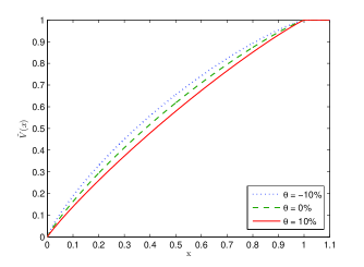
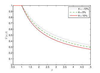
Figure 1: The benchmark is $F(S_{T})=\beta S_{T}$, and the default parameters are $S_{0}=1$, $\sigma=30\%$, and $T=1$. (Top) With $\beta=1$, the maximum success probability $\widetilde{V}(x)$ increases with initial capital $x$, and plateaus at 1 when $x>S_{0}$. For any fixed success probability, a lower Sharpe ratio $\theta$ requires a lower initial capital $x$. (Bottom) With initial capital $x=1$, $\widetilde{V}(x;\beta)$ takes value 1 and then decreases to 0 as $\beta$ increases to infinity. Observe that $\widetilde{V}(x;\beta)$ is not simply convex or concave even over the range $[0.5,5]$ of $\beta$, and converges to 0 as $\beta\to\infty$ according to (3.7).

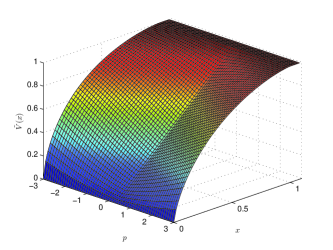
Figure 2: Outperformance probability surface over leverage $p$ and initial capital $x$. For any fixed $x$, the probability $\widetilde{V}(x)$ increases as leverage $p$ increases/decreases from zero. This means that highly leveraged ETFs are easier benchmarks to beat.

3.3 A Stochastic Factor Model

Let $(W,\hat{W})$ be a two-dimensional standard Brownian motion on $(\Omega,\mathcal{F},\mathbb{P},(\mathcal{F}_{t})_{0\leq t\leq T})$. We consider a liquid stock whose price follows the SDE:

$$dS_{t}=S_{t}\sigma(Y_{t})(\theta(Y_{t})dt+dW_{t}),$$ (3.28)

where $\theta$ is the Sharpe ratio function, and the stochastic factor $Y$ follows

$$dY_{t}=b(Y_{t})dt+c(Y_{t})(\rho dW_{t}+\sqrt{1-\rho^{2}}d\hat{W}_{t}).$$ (3.29)

This is a standard stochastic factor/volatility model that can be found in, among others, [25, 31]. The parameter $\rho\in(-1,1)$ accounts for the correlation between $S$ and $Y$.

With initial capital $x$ and strategy $\pi\in\mathcal{A}(x)$, the wealth process satisfies

$$dX^{x,\pi}_{t}=\pi_{t}S_{t}\sigma(Y_{t})(\theta(Y_{t})dt+dW_{t}).$$ (3.30)

Let $\Lambda$ be the collection of all $\mathcal{F}_{t}$ progressively measurable process $\lambda:(0,T)\times\Omega\to\mathbb{R}$ satisfying $\int_{0}^{T}\lambda^{2}_{t}dt<\infty$ $\mathbb{P}$-a.s., and denote the set of all Radon-Nikodym densities of equivalent martingale measures by $\mathcal{Z}=\{\tilde{Z}^{\lambda}_{T}:\lambda\in\Lambda\}$ where

$$\tilde{Z}^{\lambda}_{T}=\exp\Big{\{}-\frac{1}{2}\int_{0}^{T}\!\theta^{2}(Y_{t})dt-\int_{0}^{T}\!\theta(Y_{t})dW_{t}-\frac{1}{2}\int_{0}^{T}\!\lambda^{2}_{t}dt-\int_{0}^{T}\!\lambda_{t}d\hat{W}_{t}\Big{\}}.$$ (3.31)

The process $\lambda$ is commonly referred to as the risk premium for the non-traded Brownian motion $\hat{W}$. In particular, the choice of $\lambda=0$ results in the minimal martingale measure (MMM) ${\mathbb{Q}}^{0}$ (see [14]).

3.3.1 The Role of the Minimal Martingale Measure

Let us consider a benchmark of the form $F=\beta S^{\delta}_{T}$, where $\delta\in\{0,1\}$. This includes the constant and stock benchmarks. Following (3.3), we consider the optimization problem:

$$\widetilde{V}(x)=\sup_{\pi\in\mathcal{A}(x)}\mathbb{P}\{X_{T}^{x,\pi}\geq\beta S^{\delta}_{T}\}.$$ (3.32)

Proposition 3.9

Suppose $c_{1}<|\theta(y)-\delta\sigma(y)|<c_{2}$ holds for all $(y,\delta)\in\mathbb{R}\times\{0,1\}$ for some positive constants $c_{1}$ and $c_{2}$. Then, the value function $\widetilde{V}(x)$ in (3.32) is non-decreasing, continuous and concave function satisfying

$$\widetilde{V}(x)=\inf_{a\geq 0}\{xa+\mathbb{E}[(1-a\beta S_{0}^{\delta}\tilde{Z}^{{0}}_{T})^{+}]\}.$$ (3.33)

To show this, we will use the following result, which is a variation of [17, Exercise 2.3] and the proofs of (5.3) and (5.6) in [8, p.19].

Lemma 3.10

Let $B$ be a standard Brownian motion on $(\Omega,\mathcal{F},\mathbb{P},(\mathcal{F}_{t})_{0\leq t\leq T})$, and $\{a_{t},b_{t}\}_{0\leq t\leq T}$ be two ${\mathcal{F}}_{t}$-progressively measurable processes such that $\int_{0}^{T}a_{t}^{2}dt\geq\int_{0}^{T}b_{t}^{2}dt$ ${\mathbb{P}}$-a.s. Define, for $0\leq t\leq T$, the two processes

$$Z^{a}_{t}:=\exp\Big{\{}-\frac{1}{2}\int_{0}^{t}a^{2}_{u}du-\int_{t}^{t}a_{u}dB_{u}\Big{\}},\quad Z^{b}_{t}:=\exp\Big{\{}-\frac{1}{2}\int_{0}^{t}b^{2}_{u}du-\int_{t}^{t}b_{u}dB_{u}\Big{\}}.$$

For any convex function $\psi:\mathbb{R}\to\mathbb{R}$, we have

$$\mathbb{E}[\psi(Z^{a}_{T})]\geq\mathbb{E}[\psi(Z^{b}_{T})].$$ (3.34)

Proof: Define

$$\tau^{a}(s):=\inf\{t\geq 0:\int_{0}^{t}a^{2}_{u}du>s\},\qquad\tau^{b}(s):=\inf\{t\geq 0:\int_{0}^{t}b^{2}_{u}du>s\}.$$

Then, since the processes $\int_{0}^{t}a_{u}dB_{u}$ and $\int_{0}^{t}b_{u}dB_{u}$ are local martingales, the time-changed processes

$$B_{t}^{a}:=\int_{0}^{\tau^{a}(t)}a_{u}dB_{u},\qquad B_{t}^{b}:=\int_{0}^{\tau^{b}(t)}b_{u}dB_{u}$$

are two standard Brownian motions adapted to the time-changed filtrations $\{\mathcal{F}_{\tau^{a}(t)}:t>0\}$ and $\{\mathcal{F}_{\tau^{b}(t)}:t>0\}$ under the same probability space $(\Omega,\mathcal{F},\mathbb{P})$, respectively. Define

$$T^{a}:=\int_{0}^{T}a_{u}^{2}du,\qquad T^{b}:=\int_{0}^{T}b_{u}^{2}du.$$

Then, it follows that $\tau^{a}(T^{a})=\tau^{b}(T^{b})=T$, and

$$\mathbb{E}[\psi(Z_{T}^{a})]=\mathbb{E}[\psi(\exp\{-\frac{1}{2}T^{a}-B^{a}_{T^{a}}\})],\quad\mathbb{E}[\psi(Z_{T}^{b})]=\mathbb{E}[\psi(\exp\{-\frac{1}{2}T^{b}-B^{b}_{T^{b}}\})].$$

With the martingale $\exp\{-\frac{1}{2}t-B^{a}_{t}\}$ and convex function $\psi$, Jensen’s inequality implies that $\psi(\exp\{-\frac{1}{2}t-B^{a}_{t}\})$ is a submartingale. Also observe that $T^{a}\geq T^{b}$ almost surely in $\mathbb{P}$. Therefore, $\mathbb{E}[\psi(Z_{T}^{a})]=\mathbb{E}[\psi(\exp\{-\frac{1}{2}T^{a}-B^{a}_{T^{a}}\})]\geq\mathbb{E}[\psi(\exp\{-\frac{1}{2}T^{b}-B^{a}_{T^{b}}\})]=\mathbb{E}[\psi(Z_{T}^{b})].$ $\Box$

Next, we proceed to prove Proposition 3.9.

Proof: Applying Theorem 3.5, the associated randomized hypothesis testing is given by

$$\widetilde{V}(x)=\inf_{a\geq 0,\lambda\in\Lambda}\{xa+\mathbb{E}[(1-a\beta\tilde{Z}^{\lambda}_{T}S_{T}^{\delta})^{+}]\},$$

where according to (3.28) and (3.31),

$$\tilde{Z}^{\lambda}_{T}S_{T}^{\delta} =S_{0}^{\delta}\exp\Big{\{}\delta(\delta-1)\int_{0}^{T}\frac{\sigma^{2}(Y_{t})}{2}dt\Big{\}}\cdot\exp\Big{\{}-\int_{0}^{T}\frac{\lambda^{2}_{t}}{2}dt-\int_{0}^{T}\lambda_{t}d\hat{W}_{t}\Big{\}}$$

$$\cdot\exp\Big{\{}-\int_{0}^{T}\frac{(\delta\sigma(Y_{t})-\theta(Y_{t}))^{2}}{2}dt-\int_{0}^{T}(\theta(Y_{t})-\delta\sigma(Y_{t}))dW_{t}\Big{\}}.$$ (3.35)

Note that for $\delta\in\{0,1\}$, $\tilde{Z}^{\lambda}S^{\delta}$ can be rewritten as

$$\tilde{Z}^{\lambda}_{T}S_{T}^{\delta}=S_{0}^{\delta}\exp\Big{\{}-\int_{0}^{T}\frac{\alpha_{t}^{2}+\lambda_{t}^{2}}{2}dt-\int_{0}^{T}\sqrt{\alpha_{t}^{2}+\lambda_{t}^{2}}dB_{t}\Big{\}},$$

where $\alpha_{t}:=\theta(Y_{t})-\delta\sigma(Y_{t})$ and $B_{t}$ is a standard Brownian motion defined by

$$dB_{t}=\frac{-\alpha_{t}dW_{t}-\lambda_{t}d\hat{W}_{t}}{\sqrt{\alpha_{t}^{2}+\lambda_{t}^{2}}}.$$

Hence $\tilde{Z}^{\lambda}S^{\delta}$ is in fact a ${\mathbb{P}}$-martingale for $\delta\in\{0,1\}$. In view of Lemma 3.10, for any fixed $a\geq 0$, it is optimal to take $\hat{\lambda}\equiv 0$. Since $\alpha_{t}^{2}$ is bounded positive process away from zero, applying Proposition A.5 and Girsanov theorem, we have $\mathbb{P}\{-\int_{0}^{T}\frac{1}{2}\alpha_{t}^{2}dt-\int_{0}^{T}\alpha_{t}dB_{t}=c\}=0$, and hence $\mathbb{P}\{\tilde{Z}^{\hat{\lambda}_{T}}S_{T}^{\delta}=c\}=0$ holds for any constant $c$ and $\delta\in\{0,1\}$. To this end, we verified the second condition of Theorem 3.5, and conclude $\widetilde{V}(x)=V_{1}(x)=V(x)$ together with Proposition 3.3. $\Box$

Proposition 3.9 shows that among all candidate EMMs the MMM ${\mathbb{Q}}^{0}$ is optimal for $\widetilde{V}(x)$. In other words, when the benchmark is a constant or the stock $S_{T}$, the objective to maximize the outperformance probability induces the investor to assign a zero risk premium ($\lambda_{t}=0$) for the second Brownian motion $\hat{W}$ under the stochastic factor model (3.28)-(3.29). Interestingly, this is true for all choices of $\theta$, $\sigma$, $b$, $c$ and $\rho$ for $(S,Y)$. Furthermore, if $\alpha_{t}=\theta(Y_{t})-\delta\sigma(Y_{t})$ is constant, then the expectation in (3.33) and hence the success probability $\widetilde{V}(x)$ can be computed explicitly.

Corollary 3.11

Suppose $\theta(Y_{t})-\delta\sigma(Y_{t})=\alpha$ for some constant $\alpha\in{\mathbb{R}}\setminus\{0\}$. Then, $\widetilde{V}(x)$ is given by

$$\begin{array}[]{ll}\widetilde{V}(x)&=\left\{\begin{array}[]{ll}1,&\hbox{ if }x\geq\beta S^{\delta}_{0}\\ x\hat{a}+\Phi\big{(}d_{2}(\hat{a};-\alpha)\big{)}-\hat{a}S^{\delta}_{0}\Phi\big{(}d_{1}(\hat{a};-\alpha)\big{)},&\hbox{ if }x<\beta S^{\delta}_{0}\\ \end{array}\right.\end{array}$$ (3.36)

where $d_{1}$ and $d_{2}$ are given in (3.25) and $\hat{a}$ in (3.27).

3.3.2 General Benchmark and the HJB Characterization

More generally, let us consider a stochastic benchmark in the form $F=f(S_{T},Y_{T})$ for some measurable function $f$. The outperformance portfolio optimization is given by

$$\widetilde{V}(t,s,x,y)=\sup_{\pi\in\mathcal{A}(x)}\mathbb{P}^{t,s,x,y}\{X^{x,\pi}_{T}\geq f(S_{T},Y_{T})\},$$ (3.37)

where the notation $\mathbb{P}^{t,s,x,y}\{\cdot\}=\mathbb{P}\{\cdot\ |S_{t}=s,X_{t}=x,Y_{t}=y\}$. We define:

$$U(t,s,y,z):=\inf_{\lambda\in\Lambda_{t}}\mathbb{E}^{t,s,y}[(1-Z^{z,\lambda}_{T}f(S_{T},Y_{T}))^{+}],$$ (3.38)

where $\mathbb{E}^{t,s,y}[\ \cdot\ ]=\mathbb{E}[\ \cdot\ |S_{t}=s,Y_{t}=y]$, and $Z$ is given by

$$Z^{z,\lambda}_{u}=z+\int_{t}^{u}Z^{z,\lambda}_{\nu}(-\theta(Y_{\nu})dW_{\nu}-\lambda_{\nu}d\hat{W}_{\nu}).$$ (3.39)

In view of Theorem 3.5, if $\mathbb{P}\{Z_{T}^{a,\lambda}f(S_{T},Y_{T})=1\}=0$ for all $a$, then we have

$$\widetilde{V}(t,s,x,y) =\inf_{a\geq 0}\{xa+\inf_{\lambda\in\Lambda_{t}}\mathbb{E}^{t,s,y}[(1-aZ^{1,\lambda}_{T}f(S_{T},Y_{T}))^{+}]\}$$

$$=\inf_{a\geq 0}\{xa+\inf_{\lambda\in\Lambda_{t}}\mathbb{E}^{t,s,y}[(1-Z^{a,\lambda}_{T}f(S_{T},Y_{T}))^{+}]\}$$ (3.40)

$$=\inf_{a\geq 0}\{xa+U(t,s,y,a)\}.$$ (3.41)

We shall derive the associated HJB PDE for $U$. To this end, we define, for any scalar $\lambda\in{\mathbb{R}}$, the differential operator

$${\mathcal{L}}^{\lambda}w =s\theta(y)\sigma(y)w_{s}+\frac{1}{2}s^{2}\sigma^{2}(y)w_{ss}+b(y)w_{y}+\frac{1}{2}c^{2}(y)w_{yy}$$

$$+\frac{1}{2}(\theta^{2}(y)+\lambda^{2})z^{2}w_{zz}+s\sigma(y)c(y)\rho w_{sy}$$

$$-sz\sigma(y)\theta(y)w_{sz}+zc(y)(-\theta(y)\rho-\lambda\sqrt{1-\rho^{2}})w_{yz}.$$

Define the domains $\mathcal{O}=(0,\infty)\times(-\infty,\infty)\times(0,\infty)$, $\mathcal{O}_{T}=(0,T)\times\mathcal{O}$. Also, denote by $C^{2,1}(\mathcal{O}_{T})$ the collection of all functions on $\mathcal{O}_{T}$ which is continuously differentiable in $t$ and continuously twice differentiable in $(s,y,z)$.

First, we have the standard verification theorem, which is based on the existence of a classical solution.

Theorem 3.12

If there exists $w\in C^{2,1}(\mathcal{O}_{T})\cap C(\overline{\mathcal{O}}_{T})$ satisfying the PDE:

$$w_{t}+\inf_{\lambda\in\mathbb{R}}{\mathcal{L}}^{\lambda}w=0,$$ (3.42)

with $w(T,s,y,z)=(1-zf(s,y))^{+}$, then $w\leq U$ holds on $\mathcal{O}_{T}$. Furthermore, if there exists a pair $(\hat{Z},\hat{\lambda})$ of (3.39), where $\hat{\lambda}$ is a feedback form of $\hat{\lambda}_{\nu}=\hat{\lambda}(\nu,S_{\nu},Y_{\nu},\hat{Z}_{\nu})$ satisfying

$${\mathcal{L}}^{\hat{\lambda}(t,s,y,z)}w(t,s,y,z)=\inf_{\lambda\in\mathbb{R}}{\mathcal{L}}^{\lambda}w(t,s,y,z)=0,$$ (3.43)

then $w=U$ holds on $\mathcal{O}_{T}$.

Furthermore, if $\mathbb{P}\{Z_{T}^{a,\lambda}f(S_{T},Y_{T})=1\}=0$ for all $a$, then there exists $\hat{a}=\hat{a}(t,s,x,y)$ solves

$$\mathbb{E}^{t,s,y}[Z^{\hat{a},\hat{\lambda}}_{T}f(S_{T},Y_{T})I_{\{Z^{\hat{a},\hat{\lambda}}_{T}f(S_{T},Y_{T})<1\}}]=\hat{a}x,$$ (3.44)

and

$$\widetilde{V}(t,s,x,y)=\mathbb{P}^{t,s,x,y}\{Z^{\hat{a},\hat{\lambda}}_{T}f(S_{T},Y_{T})<1\}.$$ (3.45)

Proof: We follow the standard argument of verification theorem (Theorem 5.5.1 of [33]) in this below. First, for any $(S,Y,Z^{\lambda})$ with initial $(s,y,z)$ at time $t$, we have

$$w(t,s,y,z)+\mathbb{E}^{t,s,y,z}\Big{[}\int_{t}^{T}\mathcal{L}^{\lambda}w(\nu,S_{\nu},Y_{\nu},Z_{\nu})d\nu\Big{]} =\mathbb{E}^{t,s,y,z}[w(T,S_{T},Y_{T},Z_{T})]$$

$$=\mathbb{E}^{t,s,y}[(1-Z^{z,\lambda}_{T}f(S_{T},Y_{T}))^{+}].$$

The last equality above holds by terminal condition of PDE. Also observe that $\mathbb{E}^{t,s,y,z}\Big{[}\int_{t}^{T}\mathcal{L}^{\lambda}w(\nu,S_{\nu},Y_{\nu},Z_{\nu})d\nu\Big{]}$ is always non-negative, and so we have

$$w(t,s,y,z)\leq\mathbb{E}^{t,s,y}[(1-Z^{z,\lambda}_{T}f(S_{T},Y_{T}))^{+}].$$

So, we conclude $w\leq U$ by arbitrariness of $\lambda$. On the other hand, if we take $\hat{\lambda}$ of (3.43) in the above, then it yields equality, instead of inequality

$$w(t,s,y,z)=\mathbb{E}^{t,s,y}[(1-Z^{z,\lambda}_{T}f(S_{T},Y_{T}))^{+}].$$

By definition (3.38), we have right-hand side is always greater than or equal to $U$, and this implies $w\geq U$.

Applying (3.40)-(3.41), the optimizer $\hat{a}$ for $V(t,s,x,y)$ is derived from (2.8) of Theorem 2.3 with $\hat{H}=Z^{\hat{a},\hat{\lambda}}_{T}f(S_{T},Y_{T})$ and $\hat{X}=I_{\{Z^{\hat{a},\hat{\lambda}}_{T}f(S_{T},Y_{T})<1\}}$. In turn, this yields (3.44) and (3.45) via (2.10). $\Box$

Under quite general conditions, one can show that $U$ of (3.38) is the unique solution of HJB equation (3.42) in the viscosity sense.

Assumption 3.13

$\theta(\cdot)$, $\mu(\cdot)$, $b(\cdot)$, $\sigma(\cdot)$, $f(\cdot,\cdot)$ and $c(\cdot)$ are all Lipschitz continuous.

Proposition 3.14

Under Assumption 3.13, the dual function $U$ in (3.38) is the unique bounded continuous viscosity solution of (3.42) with datum $w(T,s,y,z)=(1-zf(s,y))^{+}$ for all $(s,y,z)\in\mathcal{O}$.

Proof: First, it can be shown that $U$ is the viscosity sub-solution (resp. supersolution) using the Feynman-Kac formula on its super (resp. sub) test functions. For details, we refer to the similar proof in [4, Appendix].

For uniqueness, we transform the domain from $\mathcal{O}$ to $\mathbb{R}$, by taking $x=(x_{1},x_{2},x_{3}):=(e^{s},y,e^{z})$ and defining $v(t,x):=w(t,s,y,z)$. Then, (3.42) is equivalent to

$$\inf_{\lambda\in\mathbb{R}}(v_{t}+\widetilde{L}^{\lambda}v)(t,x)=0,\ (t,x)\in(0,T)\times\mathbb{R}^{3},$$ (3.46)

where

$$\widetilde{L}^{\lambda}v =\displaystyle\frac{1}{2}\sigma^{2}(x_{2})v_{x_{1}x_{1}}+\frac{1}{2}c^{2}(x_{2})v_{x_{2}x_{2}}+\frac{1}{2}(\theta^{2}(x_{2})+\lambda^{2})v_{x_{3}x_{3}}$$

$$+\sigma(x_{2})c(x_{2})\rho v_{x_{1}x_{2}}-\sigma(x_{2})\theta(x_{2})v_{x_{1}x_{3}}+c(x_{2})(-\rho\theta(x_{2})-\sqrt{1-\rho^{2}}\lambda)v_{x_{2}x_{3}}$$

$$+(\theta(x_{2})-\frac{1}{2}\sigma(x_{2}))\sigma(x_{2})v_{x_{1}}+b(x_{2})v_{x_{2}}-\frac{1}{2}(\theta^{2}(x_{2})+\lambda^{2})v_{x_{3}}.$$

Now put in the standard form (3.46), the uniqueness of solution $v$, and thus $w$, follows from the comparison result in [15, Theorem 4.1]. $\Box$

4 Conclusions and Extensions

We have studied the outperformance portfolio optimization problem in complete and incomplete markets. The mathematical model is related to the generalized composite pure and randomized hypothesis testing problems. We established the connection between these two testing problems and then used it to address our portfolio optimization problem. The maximal success probability exhibits special properties with respect to benchmark scaling, while the outperformance portfolio optimization does not enjoy economy of scale. In various cases, we obtained explicit solutions to the outperformance portfolio optimization problem. In the stochastic volatility model, we showed the special role played by the minimal martingale measure. With the general benchmark, HJB characterization is available for the outperformance probability. An alternative approach is the characterization via BSDE solution for its dual representation (see [23, 24]).

There are a number of avenues for future research. Most naturally, one can consider quantile hedging under other incomplete markets, with specific market frictions and trading constraints. Another extension involves claims with cash flows over different (random) times, rather than a payoff at a fixed terminal time, such as American options and insurance products.

On the other hand, the composite nature of the hypothesis testing problems lends itself to model uncertainty. To illustrate this point, let’s consider a trader who receives $x$ from selling a contingent claim with terminal random payoff $F\in[0,K]$ at time $T$. The objective is to minimize the risk of the terminal liability $-F$ in terms of Average Value at Risk

$$AVaR(-F) :=\max_{\mathbb{Q}\in\mathcal{Q}_{\lambda}}\mathbb{E}^{\mathbb{Q}}[F]$$ (4.1)

subject to $$\inf_{Z\in\mathcal{Z}}\mathbb{E}[ZF]\geq x,$$

where the set of measures $\mathcal{Q}_{\lambda}:=\{\mathbb{Q}\ll\mathbb{P}\,\Big{|}\,\frac{d\mathbb{Q}}{d\mathbb{P}}\leq\frac{1}{\lambda},\ \mathbb{P}-a.s.\}$ for $\lambda\in(0,1]$.

In fact, we can convert this problem into a randomized composite hypothesis testing problem as in (2.4). To this end, we define $X:=(K-F)/K$ and then write $AVaR(-F)=K-KV_{\lambda}(x)$, where $V_{\lambda}(x)$ solves

$$V_{\lambda}(x) =\sup_{X\in\mathcal{X}}\inf_{\mathbb{Q}\in\mathcal{Q}_{\lambda}}\mathbb{E}^{\mathbb{Q}}[X]$$

subject to $$\sup_{Z\in\mathcal{Z}}\mathbb{E}[ZX]\leq\frac{K-x}{K}.$$

Following the analysis in this paper, one can obtain the properties of the value function $V_{\lambda}(x)$ as well as the structure of the optimal solution.

Finally, the outperformance portfolio optimization problem in Section 3 is formulated with respect to a fixed reference measure $\mathbb{P}$. This corresponds to applying the theoretical results of Section 2 with the set $\mathcal{G}=\{1\}$; cf. the proofs of Proposition 3.3 and Theorem 3.5. It is also possible to incorporate model uncertainty by replacing the reference measure $\mathbb{P}$ by a class of probability measures $\mathcal{M}$. In this setup, the portfolio optimization problem becomes

$${V}_{\mathcal{M}}(x):=\sup_{\pi\in\mathcal{A}(x)}\inf_{\mathbb{M}\in\mathcal{M}}\mathbb{M}\{X^{x,\pi}_{T}\geq{F}\},\qquad x\geq 0.$$

This is a special case of the hypothesis testing problems discussed in Section 2, where the original set $\mathcal{G}$ can be interpreted as the set containing the Radon-Nikodym densities $d\mathbb{M}/d\mathbb{P}$ with $\mathbb{M}\in\mathcal{M}$. For related studies on the robust quantile hedging problem, we refer to [29, 30].

Acknowledgement

The authors would like to thank two anonymous referees for their insightful remarks, as well as Jun Sekine, Birgit Rudloff and James Martin for their helpful discussions. Tim Leung’s work is partially supported by NSF grant DMS-0908295. Qingshuo Song’s work is partially supported by SRG grant 7002818 and GRF grant CityU 103310 of Hong Kong.

Appendix A Appendix

A.1 The Role of $co(\mathcal{H})$ in $V(x)$

In this example, we show that the representation of $V(x)$ in (2.10) does not hold if $co(\mathcal{H})$ is replaced by the smaller set $\mathcal{H}$.

Example A.1

Let $\Omega=[0,1]$ and $\mathbb{P}$ be the Lebesgue measure, i.e. $\mathbb{P}(a,b)=b-a$ for $a\leq b$. Let $\mathcal{G}=\{G\equiv 1\}$ and $\mathcal{H}=\{H_{1},H_{2}\}$ with

$$H_{1}(\omega)=I_{\{1/2\leq\omega\leq 1\}}+1,\quad H_{2}(\omega)=I_{\{0\leq\omega\leq 1/2\}}+1,\quad\omega\in\Omega.$$

For the randomized hypothesis testing problem (2.4) with $x=1$, it is easy to see (e.g. from (2.10)) that

$$V(1)=\inf_{a\geq 0}\{xa+\inf_{\mathcal{G}\times co(\mathcal{H})}\mathbb{E}[(G-aH)^{+}]\}\Big{|}_{x=1}=\frac{2}{3},$$

along with the optimizers:

$$\hat{G}=1,\quad\hat{H}=\frac{1}{2}(H_{1}+H_{2}),\quad\hat{a}=2/3.$$

In this simple example, uniqueness follows immediately.

Now, if one switches from $co(\mathcal{H})$ to $\mathcal{H}$ in (2.10), then a strictly larger value will result:

$$\inf_{a\geq 0}\{xa+\inf_{\mathcal{G}\times\mathcal{H}}\mathbb{E}[(G-aH)^{+}]\}\Big{|}_{x=1}=\frac{3}{4}>\frac{2}{3}=V(1).$$

A.2 On the Positivity of $\hat{a}$

First, we give an example where the minimizer $\hat{a}$ in Theorem 2.3 takes value zero, contrasting Proposition 3.1 and Lemma 4.3 in Cvitanić and Karatzas [8]. Then, we provide a sufficient condition for $\hat{a}>0$.

Example A.2

Let $N_{g}:=\bigcap_{G\in{\cal G}}\{G=0\}$ and $x>0$.

• If $\mathbb{P}\{N_{g}\}=1$, then $\mathbb{E}[(G-aH)^{+}]\equiv 0$ for all $G,H,a$. Thus $\hat{a}=0$ is the unique minimizer of $\{xa+\inf_{\mathcal{G}\times\mathcal{H}}\mathbb{E}[(G-aH)^{+}]\}$.

• If $0<\mathbb{P}\{N_{g}\}<1$ and $x>\sup_{H\in{\cal H}}\mathbb{E}[(HI_{N_{g}^{c}})]$, then there also exists a counter-example such that $\hat{a}=0$ minimizes $\{xa+\inf_{\mathcal{G}\times\mathcal{H}}\mathbb{E}[(G-aH)^{+}]\}$. Indeed, set ${\cal G}=\{G\}$ with $G={I_{N_{g}^{c}}}/{\mathbb{P}\{N_{g}^{c}\}}$ and ${\cal H}=\{H\}$ with $H\equiv 1$, then we have

  $$xa+\inf_{\mathcal{G}\times\mathcal{H}}\mathbb{E}[(G-aH)^{+}] =xa+\mathbb{E}[(G-zH)^{+}]$$ (A.1)

  $$=\left\{\begin{array}[]{cl}xa,&\text{if}\quad a\geq\frac{1}{P\{N_{g}^{c}\}};\\ 1+a\left(x-\mathbb{P}\{N_{g}^{c}\}\right),&\text{if}\quad 0\leq a<\frac{1}{\mathbb{P}\{N_{g}^{c}\}}.\end{array}\right.$$

  Since $x>\sup_{H\in{\cal H}}\limits\mathbb{E}[HI_{N_{g}^{c}}]=\mathbb{P}\{N_{g}^{c}\}$, $\hat{a}=0$ is the unique minimizer of (A.1). $\Box$

Proposition A.3

If

$$0<x<\sup_{\mathcal{H}}\mathbb{E}[HI_{\underset{G\in\mathcal{G}}{\cap}\{G>0\}}],$$ (A.3)

then there exists $(\hat{G},\hat{H},\hat{a},\hat{X})\in\mathcal{G}\times\overline{co(\mathcal{H})}\times(0,\infty)\times\mathcal{X}_{x}$ satisfying (2.7)-(2.9). In particular,

$$\hat{a}=\operatorname*{arg\,min}_{a\geq 0}\{xa+\inf_{\mathcal{G}\times\overline{co(\mathcal{H})}}\mathbb{E}[(G-aH)^{+}]\}>0.$$

Proof: Define the function $f_{x}(a):=xa+\inf_{\mathcal{G}\times\overline{co(\mathcal{H})}}\mathbb{E}[(G-aH)^{+}]$, which is Lipschitz continuous (see Lemma 4.1 of [8]). Since $f_{x}(0)=\inf_{\mathcal{G}}\mathbb{E}[G]\geq 0$ and is finite, and $\lim_{a\to\infty}f_{x}(a)=\infty$, there exists a finite $\hat{a}\geq 0$ that minimizes $f_{x}(a)$.

Now, suppose $\hat{a}=0$ is a minimizer of $f_{x}(a)$. Then, it follows that $f_{x}(a)\geq f_{x}(0)$, $\forall a>0$, which leads to

$$\begin{array}[]{ll}xa&\geq\displaystyle\inf_{\mathcal{G}}\mathbb{E}[G]-\inf_{\mathcal{G}\times\overline{co(\mathcal{H})}}\mathbb{E}[(G-aH)^{+}]\\ \\ \displaystyle&\geq\mathbb{E}[\tilde{G}]-\displaystyle\inf_{\overline{co(\mathcal{H})}}\mathbb{E}[(\tilde{G}-aH)^{+}]\\ \\ &\geq\displaystyle a\sup_{\overline{co(\mathcal{H})}}\mathbb{E}[HI_{\{\tilde{G}\geq aH\}}]\geq\displaystyle a\sup_{\mathcal{H}}\mathbb{E}[HI_{\{\tilde{G}\geq aH\}}].\end{array}$$ (A.9)

In (A.9), $\tilde{G}$ minimizes $\mathbb{E}[G]$ over $\mathcal{G}$, and its existence follows from convex and closedness of $\mathcal{G}$. Taking the limit $a\to 0^{+}$ yields a contradiction to (A.3):

$$x\geq\sup_{\mathcal{H}}\mathbb{E}[HI_{\{\tilde{G}>0\}}]\geq\sup_{\mathcal{H}}\mathbb{E}[HI_{\displaystyle\cap_{\mathcal{G}}\{G>0\}}].$$

Hence, we conclude that $\hat{a}>0$. $\Box$

A.3 Counter-example for Remark 2.5

Let $\Omega=\{\omega_{1},\omega_{2}\}$, $P(\{\omega_{1}\})=P(\{\omega_{2}\})=1/2$. Then, any random variable in ${\cal G},{\cal H}$ or in $\mathcal{X}_{x}$, ${\cal I}_{x}$ can be represented as a point in ${\mathbb{R}}^{2}$. Let ${\cal H}$ be line segment connecting $(2,4)$ and $(6,2)$, ${\cal G}=\{(2,2)\}$. Given $x\geq 0$, $\mathcal{X}_{x}$ is the convex quadrangle with four vertices $(0,0),(x/3,0),(x/5,2x/5)$, $(0,x/2)$ intersected with $\{(x_{1},x_{2})\ |\ 0\leq x_{1},x_{2}\leq 1\}$. For each $H=(h_{1},h_{2})\in{\cal H}$ and $X=(x_{1},x_{2})$, the constraint ${\mathbb{E}}[HX]\leq x$ implies that $\frac{h_{1}}{2}x_{1}+\frac{h_{2}}{2}x_{2}\leq x.$ It is a half-plane bounded by $h_{1}x_{1}+h_{2}x_{2}=2x$, which passes $(x/5,2x/5)$ since $h_{1}+2h_{2}=5$. Hence, we have

$$V(x)=\sup_{(x_{1},x_{2})\in\mathcal{X}_{x}}x_{1}+x_{2},\quad\text{ and }\quad V_{1}(x)=\sup_{(x_{1},x_{2})\in{\cal I}_{x}}x_{1}+x_{2},$$

where ${\cal I}_{x}=\mathcal{X}_{x}\cap\{(0,0),(0,1),(1,0),(1,1)\}$. In summary, the values are

$x$	$V(x)$	$V_{1}(x)$
$0\leq x<2$	$\frac{3}{5}x$	$0$
$2\leq x<\frac{5}{2}$	$\frac{3}{5}x$	$1$
$\frac{5}{2}\leq x<4$	$\frac{x}{3}+\frac{2}{3}$	$1$
$x\geq 4$	$2$	$2$

By inspecting the value of $V_{1}(x)$, we see that its smallest concave majorant must take value $\frac{x}{2}$ in $[0,4]$. Therefore, $V(x)$ is not the smallest concave majorant of $V_{1}(x)$.

A.4 Counter-example for Remark 2.11

With reference to Theorem 2.3, we show via an example that one cannot remove the independence requirement when ${\mathcal{G}}$ and $H$ are not singletons.

Example A.4

Let $\Omega=\{0,1\}\times[0,1]$, $\mathcal{F}_{T}=\mathcal{B}(\Omega)$. Let $\mu$ be the Lebesgue measure on $[0,1]$. Define $\mathbb{P}$ by

$$\mathbb{P}(\{0\}\times A)=\mathbb{P}(\{1\}\times A)=\frac{1}{2}\mu(A),\quad\forall A\in\mathcal{B}([0,1]).$$

Let $H_{0}:\{0,1\}\to\mathbb{R}$ be of $H_{0}(0)=1/2$ and $H_{0}(1)=3/2$, and $f:[0,1]\to\mathbb{R}$ as an arbitrarily fixed probability density function. Define the set

$$\mathcal{H}=\{H:\Omega\to\mathbb{R}:H(\alpha,a)=H_{0}(\alpha)f(a),~{}(\alpha,a)\in\Omega\}$$

and singleton $\mathcal{G}=\{G\equiv 1\}$. Let $U$ be a uniform random variable on $(\Omega,\mathcal{F}_{T},\mathbb{P})$, such that $\mathbb{P}\{U\leq a\}=a$ for $a\in[0,1]$.

The pure hypothesis testing problem is

$$V_{1}=\sup_{A\in\mathcal{F}_{T}}\mathbb{E}[I_{A}]$$

subject to

$$\sup_{H\in\mathcal{H}}\mathbb{E}[HI_{A}]\leq 1/2.$$

Direct computation gives the success set $\hat{A}=\{0\}$ and the value of pure hypothesis test $V_{1}=1/2$. On the other hand, the randomized hypothesis testing problem

$$V=\sup_{X\in\mathcal{X}}\mathbb{E}[X]$$

subject to

$$\sup_{H\in\mathcal{H}}\mathbb{E}[HX]\leq 1/2.$$

We find that $\hat{H}(\alpha,a)=H_{0}(\alpha)$ and $\hat{X}=I_{\{\alpha=0\}}+1/3I_{\{\alpha=1\}}$ solve this randomized hypothesis test with the optimal value $V=2/3$.

This shows that the values of pure and randomized hypothesis tests are different. If one were to construct an indicator version of the randomized test as in (2.22), namely,

$$\bar{X}:=I_{\{\alpha=0\}}+I_{\{\alpha=1\}}I_{\{U<1/3\}}.$$

Although this test $\bar{X}$ still satisfies $\mathbb{E}[\hat{H}\bar{X}]=1/2$, it in fact does not solve either pure or randomized hypothesis test. Indeed, for $\tilde{H}(\alpha,a)=H_{0}(\alpha)\cdot(3I_{a<1/3})\in{\mathcal{H}}$, we observe the violation: $\mathbb{E}[\tilde{H}\bar{X}]=1>1/2$.

A.5 A property on non-degenerate martingale

On the probability space $(\Omega,\mathcal{F},\mathbb{P})$ with filtration $(\mathcal{F}_{t})_{0\leq t\leq 1}$, we denote by $W$ to be a standard Brownian motion. Let $Y$ be a $({\mathbb{P}},{\mathcal{F}}_{t})$-martingale defined by

$$Y_{t}=\int_{0}^{t}\sigma_{r}dW_{r},\quad t\in[0,1].$$

where $\sigma_{t}$ is bounded $\mathcal{F}_{t}$-adapted process.

Proposition A.5

Assume $c<\sigma_{t}<C$ for some positive constants $c$ and $C$, then

$$\mathbb{P}\{Y_{1}=b\}=0$$

for all constant $b$.

To prove this proposition, we will use following two facts. We define $f:\mathbb{R}^{+}\times\mathbb{R}^{+}\times\mathbb{R}\mapsto[0,1]$ by

$$f(x,y,u)=\mathbb{P}\{W_{t}=u\hbox{ for some }t\in(x,y)\}.$$

1. By direct computation, one can have

   $$\sup_{u\in\mathbb{R}}f(x,y,u)=f(x,y,0)<1.$$

2. By a time-change argument, we have

   $$f(\lambda x,\lambda y,u)=f(x,y,\frac{u}{\sqrt{\lambda}}),\quad\forall\lambda>0.$$

Now we are ready to present the proof of Proposition A.5.

Proof: Since $Y$ is a continuous process,

$$\{Y_{1}=b\}\in\sigma(\{\mathcal{F}_{t}:t<1\})=:\mathcal{F}_{1^{-}}.$$

By Levy’s zero one law, we have

$$I_{\{Y_{1}=b\}}=\lim_{t\uparrow 1}\mathbb{P}\{Y_{1}=b|\mathcal{F}_{t}\},\quad a.s.$$

Therefore, it is enough to show that there exists $a\in(0,1)$ such that

$$\mathbb{P}\{Y_{1}=b|\mathcal{F}_{t}\}<a<1,~{}~{}\forall t\in(0,1).$$

Note that, the martingale $(Y_{s}|Y_{t}=u:s>t)$ has the same distribution as a time-changed Brownian motion starting from state $u$. Together with $c^{2}(1-t)\leq\int_{t}^{1}\sigma_{r}^{2}dr\leq C^{2}(1-t)$, we have for some standard Brownian motion $B$ that

$$\mathbb{P}\{Y_{1}=b|Y_{t}=u\} =\mathbb{P}\{B_{r}=b-u,\hbox{ for some }r\in(c^{2}(1-t),C^{2}(1-t))\}$$

$$=f(c^{2},C^{2},\frac{b-u}{\sqrt{1-t}})\leq f(c^{2},C^{2},0).$$

Since $f(c^{2},C^{2},0)$ is independent of $t$, and strictly less than $1$, we can simply take $a=f(c^{2},C^{2},0)$. $\Box$

To this end, one may wonder whether the condition on $\sigma$ in Proposition A.5 can be relaxed to $\sigma_{t}>0$ a.s. $\forall t$. The answer is no, as shown by the counter-example in [19].

References

• [1] M. Avellaneda and S. Zhang: Path-dependence of leveraged ETF returns. SIAM J. Financ. Math. 1, 586–603 (2010)
• [2] E. Bayraktar, Y.-J. Huang, and Q. Song: Outperforming the market portfolio with a given probability. Ann. Appl. Probab. 22, 1465-1494 (2011)
• [3] P. Billingsley: Convergence of probability measures. 2nd ed., Wiley Series in Probability and Statistics: Probability and Statistics. John Wiley & Sons, New York (1999)
• [4] E. Bayraktar, Q. Song, and J. Yang: On the continuity of stochastic control problems on bounded domains. Stoch. Analysis Appl. 29, 48–60 (2011)
• [5] W. Brannath and W. Schachermayer: A bipolar theorem for $L^{0}_{+}(\Omega,\mathcal{F},\mathbb{P})$. In Séminaire de Probabilités, XXXIII, vol. 1709 of Lecture Notes in Math., pp.349–354. Springer, Berlin (1999)
• [6] S. Browne: Reaching goals by a deadline: digital options and continuous time active portfolio management. Adv. Appl. Probab. 31, 551–577 (1999)
• [7] J. Cvitanić: Minimizing expected loss of hedging in incomplete and constrained markets. SIAM J. Control Optim. 38, 1050–1066 (2000)
• [8] J. Cvitanić and I. Karatzas: Generalized Neyman-Pearson lemma via convex duality. Bernoulli 7, 79–97 (2001)
• [9] F. Delbaen and W. Schachermayer: The mathematics of arbitrage. Springer Finance. Springer-Verlag, Berlin, 2006
• [10] F. Delbaen and W. Schachermayer: A general version of the fundamental theorem of asset pricing. Math. Ann. 300, 463–520 (1994)
• [11] N. El Karoui and M. Quenez: Dynamic programming and pricing of contingent claims in an incomplete market. SIAM J. Control Optim. 33, 29–66 (1995)
• [12] H. Föllmer and P. Leukert: Quantile hedging. Finance Stoch. 3, 251–273 (1999)
• [13] H. Föllmer and A. Schied: Convex measures of risk and trading constraints. Finance Stoch. 6, 429–447 (2002)
• [14] H. Föllmer and M. Schweizer: Hedging of contingent claims under incomplete information, Applied Stochastic Analysis, Stochastics Monographs (M.H.A. Davis and R.J. Elliot, eds.), vol. 5, Gordon and Breach, London/New York, 1990, pp.389 – 414
• [15] Y. Giga, S. Goto, H. Ishii, and M.-H. Sato: Comparison principle and convexity preserving properties for singular degenerate parabolic equations on unbounded domains, Indiana Univ. Math. J. 40, 443–470 (1991)
• [16] R. Jarrow: Understanding the risk of leveraged ETFs. Finance Research Letters 7, 135–139 (2010)
• [17] M. Jeanblanc, M. Yor, and M. Chesney: Mathematical methods for financial markets. Springer Finance, London (2009)
• [18] I. Karatzas and S. Shreve: Methods of mathematical finance. Springer, New York (1998)
• [19] A non-degenerate martingale, MathOverflow, website (version: 2011-12-24): http://mathoverflow.net/questions/84216 .
• [20] R. N. Krutchenko and A. V. Melnikov: Trends in methematics: Workshop of the mathematical finance research project, Konstaz, Germany, October 5-7, 2000, Birkhauser Verlag Basel, Switzerland (2001)
• [21] E.L. Lehmann and J.P. Romano: Testing Statistical Hypotheses, 3rd ed. Springer, New York (2005)
• [22] T. Leung, Q. Song, and J. Yang: Generalized Hypothesis Testing and Maximizing the Success Probability in Financial Markets, Proceedings of the International Conference on Business Intelligence and Financial Engineering (ICBIFE), 2011.
• [23] J. Ma and J. Yong: Forward-backward stochastic differential equations and their applications, volume 1702 of Lecture Notes in Mathematics. Springer-Verlag, Berlin (1999)
• [24] J. Ma and J. Zhang: Representation theorems for backward stochastic differential equations. Ann. Appl. Probab. 12, 1390–1418 (2002)
• [25] M. Romano and N. Touzi: Contingent claims and market completeness in a stochastic volatility model. Math. Finance 7, 399–410 (1997)
• [26] B. Rudloff: Convex hedging in incomplete markets. Appl. Math. Finance 14, 437–452 (2007)
• [27] B. Rudloff and I. Karatzas: Testing composite hypotheses via convex duality, Bernoulli 16, 1224–1239 (2010)
• [28] A. Schied: On the Neyman-Pearson problem for law-invariant risk measures and robust utility functionals. Ann. Appl. Probab. 14, 1398–1423 (2004)
• [29] A. Schied: Optimal investments for robust utility functionals in complete market models. Math. Oper. Res. 30, 750–764 (2005)
• [30] J. Sekine: On a robustness of quantile-hedging: complete market’s case, Asia-Pacific Finan. Markets 6, 195–201 (1999)
• [31] R. Sircar and T. Zariphopoulou: Bounds and asymptotic approximations for utility prices when volatility is random. SIAM J. Control Optim. 43, 1328–1353 (2005)
• [32] G. Spivak and J. Cvitanić: Maximizing the probability of a perfect hedge. Ann. Appl. Probab. 9, 1303–1328 (1999)
• [33] J. Yong and X.-Y. Zhou: Stochastic controls: Hamiltonian systems and HJB equations, Springer, New York (1999)