The Fixed Point of the Composition of Derivatives

Abstract

We give an affirmative answer to a question of K. Ciesielski by showing that the composition $f\circ g$ of two derivatives $f,g:[0,1]\to[0,1]$ always has a fixed point. Using Maximoff’s theorem we obtain that the composition of two $[0,1]\to[0,1]$ Darboux Baire-1 functions must also have a fixed point.

Introduction

In [4] R. Gibson and T. Natkaniec mentioned the question of K. Ciesielski, which asks whether the composition $f\circ g$ of two derivatives $f,g:[0,1]\to[0,1]$ must always have a fixed point. Our main result is an affirmative answer to this question. (An alternative proof has also been found by M. Csörnyei, T. C. O’Neil and D. Preiss, see [3].)

Theorem 1.

Let $f$ and $g:[0,1]\to[0,1]$ be derivatives. Then $f\circ g$ has a fixed point.

Since any bounded approximately continuous function is a derivative (see e.g. [1]) we get the following:

Corollary 2.

Let $f$ and $g:[0,1]\to[0,1]$ be approximately continuous functions. Then $f\circ g$ has a fixed point.

Now suppose that $f,g:[0,1]\to[0,1]$ are Darboux Baire-1 functions. Then, by Maximoff’s theorem ([5], see also in [6]), there exist homeomorphisms $h,k:[0,1]\to[0,1]$ such that $f\circ h$ and $g\circ k$ are approximately continuous functions. Then clearly $\tilde{f}=k^{\textrm{-}1}\circ f\circ h$ and $\tilde{g}=h^{\textrm{-}1}\circ g\circ k$ are also $[0,1]\to[0,1]$ approximately continuous functions and $f\circ g$ has a fixed point if and only if $\tilde{f}\circ\tilde{g}$ has a fixed point. Thus from Corollary 2 we get the following:

Corollary 3.

Let $f$ and $g:[0,1]\to[0,1]$ be Darboux Baire-1 functions. Then $f\circ g$ has a fixed point.

Preliminaries

We shall denote the square $[\textrm{-}1,2]\times[\textrm{-}1,2]$ by $Q$. The partial derivatives of a function $h:\mathbb{R}^{2}\to\mathbb{R}$ with respect to the $i$-th variable ($i=1,2$) will be denoted by $\partial_{i}h$. The sets $\{h=c\}$, $\{h\neq c\}$, $\{h>c\}$, etc.(???) will denote the appropriate level sets of the function $h$. The notations $\operatorname{cl}A,\operatorname{int}A$ and $\partial A$ stand for the closure, interior and boundary of a set $A$, respectively. By component we shall always mean connected component.

1 Skeleton of the proof of Theorem 1

Let $f,g:[0,1]\to[0,1]$ be the derivatives of $F$ and $G$, respectively. We can extend $F$ and $G$ linearly to the complement of the unit interval such that they remain differentiable and such that the derivatives of the extended functions are still between 0 and 1. Therefore we may assume that $f$ and $g$ are derivatives defined on the whole real line and $0\leq f,g\leq 1$.

The key step of the proof is the following. Let

$$H(x,y)=F(x)+G(y)-xy\ \ \ (\ (x,y)\in\mathbb{R}^{2}\ ),$$ (1)

$\textrm{where }F^{\prime}=f,\ G^{\prime}=g:\mathbb{R}\to[0,1]\textrm{ are derivatives}.$

Then $H$ is differentiable as a function of two variables, and its gradient is

$$H^{\prime}(x,y)=(f(x)-y,g(y)-x).$$ (2)

Thus the gradient vanishes at $(x_{0},y_{0})$ if and only if $x_{0}$ is a fixed point of $g\circ f$ and $y_{0}$ is a fixed point of $f\circ g$. Moreover, the gradient cannot be zero outside the closed unit square, since $0\leq f,g\leq 1$. Therefore it is enough to prove that there exists a point in $\mathbb{R}^{2}$ where the gradient vanishes.

We argue by contradiction, so throughout the paper we shall suppose that the gradient of $H$ nowhere vanishes.

Let us now examine the behavior of $H$ on the edges of $Q$. By (2) the partial derivative $\partial_{1}H$ is clearly negative on the top edge of $Q$ and positive on the bottom edge, and similarly $\partial_{2}H$ is positive on the left edge and negative on the right edge. This implies the following.

Lemma 4.

$H$ is strictly decreasing on the top and right edges, and strictly increasing on the bottom and left edges of $Q$.

Consequently,

$$\max\left(H(\textrm{-}1,\textrm{-}1),H(2,2)\right)<\min\left(H(\textrm{-}1,2),H(2,\textrm{-}1)\right).$$

This inequality suggests that there must be a kind of ‘saddle point’ in $Q$. Therefore define

$$c=\inf\left\{d\,:\,(\textrm{-}1,\textrm{-}1)\text{ and }(2,2)\text{ are in the same component of }\{H\leq d\}\cap Q\right\}$$

as a candidate for the value of $H$ at a saddle point. At a typical saddle point $q$ of some smooth function $K:\mathbb{R}^{2}\to\mathbb{R}$ such that $K(q)=d$, the level set in a neighborhood of $q$ consists of two smooth curves intersecting each other at $q$. In Section 2 we shall prove the following theorem, which states that the level set $\{H=c\}$ behaves indeed in a similar way.

Theorem 5.

$\{H=c\}\cap Q$ intersects each edge of $Q$ at exactly one point (which is not an endpoint of the edge). Moreover, this level set cuts $Q$ into four pieces, that is $\{H\neq c\}\cap Q$ has four components, and each of these components contains one of the corners of $Q$. The values of $H$ are greater than $c$ in the components containing the top left and the bottom right corner of and less than $c$ in the components containing the bottom left and the top right corner.

This theorem suggests the picture that the level set $\{H=c\}\cap Q$ looks like the union of two arcs crossing each other, one from the left to the right and one from the top to the bottom. We are particularly interested in the existence of this ‘crossing point’, because at such a point four components of $\{H\neq c\}\cap Q$ should meet. Indeed, we shall prove the following (see Section 3).

Theorem 6.

There exists a point $p\in\{H=c\}\cap\operatorname{int}Q$ that is in the closure of more than two components of $\{H\neq c\}\cap Q$.

Remark 1.

It is in fact not much harder to see that there exists a point $p\in\{H=c\}\cap\operatorname{int}Q$ in the intersection of the closure of exactly four components.

But on the other hand we shall also prove (see Section 4) the following theorem about the local behavior of the level set.

Theorem 7.

Every $p\in\{H=c\}\cap\operatorname{int}Q$ has a neighborhood that intersects exactly two components of $\{H\neq c\}\cap Q$.

However, the last two theorems clearly contradict each other, which will complete the proof of Theorem 1.

2 Proof of Theorem 5

Recall that we defined

$$c=\inf\left\{d\,:\,(\textrm{-}1,\textrm{-}1)\text{ and }(2,2)\text{ are in the same component of }\{H\leq d\}\cap Q\right\}.$$

Lemma 8.

In fact, $c$ is a minimum; that is, $(\textrm{-}1,\textrm{-}1)\text{ and }(2,2)$ are in the same component of $\{H\leq c\}\cap Q$.

Proof.

Let $K_{n}$ be the component of $\left\{h\leq c+1/n\right\}\cap Q$ containing both $(\textrm{-}1,\textrm{-}1)$ and $(2,2).$ Then $K_{n}$ is clearly a decreasing sequence of compact connected sets. A well known theorem (see e.g. [7, I. 9. 4]) states that the intersection of such a sequence is connected. Hence $\cap_{n}K_{n}\subset\left\{h\leq c\right\}$ is connected and contains both $(\textrm{-}1,\textrm{-}1)$ and $(2,2)$, which shows that $(\textrm{-}1,\textrm{-}1)\text{ and }(2,2)$ are in the same component of $\{H\leq c\}\cap Q$. ∎

Lemma 9.

$\max\left\{H(\textrm{-}1,\textrm{-}1),H(2,2)\right\}<c<\min\left\{H(\textrm{-}1,2),H(2,\textrm{-}1)\right\}.$

Proof.

To show $H(2,2)<c$ consider the polygon $P$ with vertices $(\textrm{-}1,2)$, $(1,2)$, $(2,1)$ and $(2,\textrm{-}1)$. Since $\partial_{1}H(x,y)=f(x)-y<0$ if $y>1$ and $\partial_{2}H(x,y)=g(y)-x<0$ if $x>0$, it is easy to check that $H$ is strictly bigger than $H(2,2)$ on the whole $P$. Therefore $P$ connects $(\textrm{-}1,2)$ and $(2,\textrm{-}1)$ in $\left\{H>H(2,2\right\}$, thus $(\textrm{-}1,\textrm{-}1)$ and $(2,2)$ cannot be in the same component of $\left\{H\leq H(2,2)\right\}$. By the previous Lemma this implies that $H(2,2)<c$. Proving that $H(\textrm{-}1,\textrm{-}1)$ is similar.

To show that $c<H(\textrm{-}1,2)$ consider the polygon $P^{\prime}$ with vertices $(\textrm{-}1,\textrm{-}1)$, $(\textrm{-}1,1)$, $(0,2)$ and $(2,2)$. Like above one can show that $H$ is strictly less than $H(\textrm{-}1,2)$ on the whole $P^{\prime}$, so denoting the maximum of $H$ on $P^{\prime}$ by $d$, we have $d<H(\textrm{-}1,2)$. Since $P^{\prime}$ connects $(\textrm{-}1,\textrm{-}1)$ and $(2,2)$ in $\{H\leq d\}\cap Q$ we also have $c\leq d$, therefore we have $c<H(\textrm{-}1,2)$. Proving that $c<H(2,\textrm{-}1)$ would be similar. ∎

The previous Lemma together with Lemma 4 clearly implies the first statement of Theorem 5: $\left\{H=c\right\}\cap Q$ intersect each edge of $Q$ at exactly one point (which is not an endpoint of the edge). Since $4$ points cut $\partial Q$ into four components we also get that $\left\{H\neq c\right\}\cap\partial Q$ has $4$ components and each of them contains a vertex of $Q$. Therefore for completing the proof of Theorem 5 we have to show that any component of $\left\{H\neq c\right\}\cap Q$ intersect $\partial Q$ and that the vertices of $Q$ belong to different components of $\left\{H\neq c\right\}\cap Q$.

The first claim is clear since if $C$ were a component of $\left\{H\neq c\right\}\cap Q$ inside $Q$ then one of the (global) extrema of $H$ on the (compact) closure of $C$ could not be on the boundary of $C$ (where $H=c$), so this would be a local extremum but a function with non-vanishing gradient cannot have a local extremum.

To prove the second claim first note that the components of $\left\{H\neq c\right\}\cap Q$ are the components of $\left\{H<c\right\}\cap Q$ and the components of $\left\{H>c\right\}\cap Q$. By the previous Lemma, $(\textrm{-}1,\textrm{-}1)$ and $(2,2)$ are in $\left\{H<c\right\}\cap Q$ while $(\textrm{-}1,2)$ and $(2,\textrm{-}1)$ are in $\left\{H>c\right\}\cap Q$, so it is enough to prove that that the opposite vertices belong to different components.

Assume that $(\textrm{-}1,\textrm{-}1)$ and $(2,2)$ are in the same component of $\left\{H<c\right\}\cap Q$. Then there is a continuous curve in $\left\{H<c\right\}\cap Q$ that connects $(\textrm{-}1,\textrm{-}1)$ and $(2,2).$ Let $d$ be the maximum of $H$ on this curve. Then on one hand $d<c$; on the other hand, $(\textrm{-}1,\textrm{-}1)\text{ and }(2,2)$ are in the same component of $\{H\leq d\}\cap Q$, so $c\leq d$, which is a contradiction.

Finally, assume that $(\textrm{-}1,2)$ and $(2,\textrm{-}1)$ are in the same components of $\left\{H>c\right\}\cap Q$. Then there is a continuous curve in $\left\{H>c\right\}\cap Q$ that connects $(\textrm{-}1,2)$ and $(2,\textrm{-}1)$, so it also separates $(\textrm{-}1,1)$ and $(2,2)$. But this is a contradiction with Lemma 8.

3 Proof of Theorem 6

The following topological lemma is surely well known. However, we were unable to find it in the literature, so we sketch a proof here.

Lemma 10.

Let $M$ be a closed subset of $Q$ and $p\neq q\in M\cap\partial Q.$ Denote by $E_{1}$ and $E_{2}$ the two connected components of $\partial Q\setminus\{p,q\}$. Then the following statements are equivalent:

• $p$ and $q$ are not in the same component of $M$.

• there are points $e_{i}\in E_{i}\ (i=1,2)$ that can be connected by a polygon in $Q\setminus M$.

Proof.

The implication (ii) $\Rightarrow$ (i) is obvious. The implication (i) $\Rightarrow$ (ii) easily follows from Zoretti’s Theorem (see [7] Ch. VI., Cor. 3.11), which states that if $K$ is a component of a compact set $M$ in the plane and $\varepsilon>0$, then there exists a simple closed polygon $P$ in the $\varepsilon$-neighborhood of $K$ that encloses $K$ and is disjoint from $M$. ∎

Now we turn to the proof of Theorem 6. Let us denote by $C_{p}$ the component of $\{H\neq c\}\cap Q$ that contains the corner $p$ of $Q$ (Theorem 5 shows that $p\in\{H\neq c\}\cap Q$). Again by Theorem 5 we have $\{H\neq c\}\cap Q=C_{(\textrm{-}1,\textrm{-}1)}\cup C_{(2,2)}\cup C_{(\textrm{-}1,2)}\cup C_{(2,\textrm{-}1)}$, and $H$ is less than $c$ in the first two and greater than $c$ in the last two components.

Proposition 11.

There exists a point $r\in\operatorname{cl}{C_{(\textrm{-}1,\textrm{-}1)}}\cap\operatorname{cl}{C_{(2,2)}}$.

Proof.

Suppose, on the contrary, that there is no such point. Then the components of $\{H\leq c\}\cap Q$ are $\operatorname{cl}{C_{(\textrm{-}1,\textrm{-}1)}}$ and $\operatorname{cl}{C_{(2,2)}}$, hence $(\textrm{-}1,\textrm{-}1)$ and $(2,2)$ are in different components. Therefore, if we apply the previous lemma to $\{H\leq c\}\cap Q$ with $p=(\textrm{-}1,\textrm{-}1)$ and $q=(2,2)$, then we obtain a polygon in $\{H>c\}\cap Q$ joining either the left or the top edge to either the right or the bottom edge of $Q$. Let us now join the endpoints of this polygon to the points $(\textrm{-}1,\textrm{-}1)$ and $(2,2)$ by two segments. By Lemma 4 these segments must also be in $\{H>c\}\cap Q$, and we thus obtain a polygon in $\{H>c\}\cap Q$ connecting $(\textrm{-}1,\textrm{-}1)$ and $(2,2)$, which contradicts Theorem 5. ∎

Our next aim is to show that such a point $r$ cannot be on the edges of $Q$. The other cases being similar we only consider the case of the left edge.

Lemma 12.

$\{[\textrm{-}1,0)\times[\textrm{-}1,2]\}\cap C_{(2,2)}=\emptyset$

Proof.

We have to prove that if $(x,y)\in[\textrm{-}1,0)\times[\textrm{-}1,2])$ such that $H(x,y)<c$, then $(x,y)\in C_{(\textrm{-}1,\textrm{-}1)}$. In order to do this, it is sufficient to show that the vertical segment $S_{1}$ between $(x,y)$ and $(x,\textrm{-}1)$ and the horizontal segment $S_{2}$ between $(x,\textrm{-}1)$ and $(\textrm{-}1,\textrm{-}1)$ together form a polygon in $\left\{H(x,y)<c\right\}$ connecting $(x,y)$ to $(\textrm{-}1,\textrm{-}1)$. But by (2) in Section 1 the partial derivative $\partial_{2}H$ is positive on $S_{1}$, thus all values of $H$ are less then $H(x,y)$ here, hence less then $c$, and $\partial_{1}H$ is positive on $S_{2}$, thus the values of $H$ here are less then $H(x,\textrm{-}1)$, which is again less than $c$. ∎

Let $r$ be a point provided by Proposition 11. If we repeat the agrument of the previous lemma for the other three edges, then we obtain that $r$ must be in the interior of $Q$. To complete the proof of Theorem 6 it is enough to show that there exists a component in which $H$ is greater than $c$ (that is either component $C_{(\textrm{-}1,2)}$ or $C_{(2,\textrm{-}1)}$) such that the closure of the component contains $r$. But $r\in\operatorname{int}Q$, and then this statement follows from the fact that the gradient of $H$ nowhere vanishes, so $H$ attains no local extremum.

4 Proof of Theorem 7

Lemma 13.

Let $x_{1},x_{2},y_{1},y_{2}\in\mathbb{R}$ be such that $x_{1}<x_{2}$ and $y_{1}<y_{2}$. Then $H(x_{1},y_{2})+H(x_{2},y_{1})-H(x_{1},y_{1})-H(x_{2},y_{2})>0$.

Proof.

Using the definition (1) of $H$, a straightforward computation shows that the value of the above sum in fact equals $(x_{2}-x_{1})(y_{2}-y_{1})>0.$ ∎

Lemma 14.

Let $(x_{0},y_{0})\in\mathbb{R}^{2}$ be such that $H(x_{0},y_{0})=0$ and $\partial_{2}H(x_{0},y_{0})\neq 0$. Then there exists $\varepsilon>0$ such that if $x_{1}\in[x_{0}-\varepsilon,x_{0}+\varepsilon]$ and $y_{1},y_{2}\in[y_{0}-\varepsilon,y_{0}+\varepsilon]$ and $H(x_{1},y_{1})=H(x_{1},y_{2})=0$ then one of the followings holds:

• $y_{1}=y_{2}=y_{0}$,

• $y_{1}<y_{0}$ and $y_{2}<y_{0}$,

• $y_{1}>y_{0}$ and $y_{2}>y_{0}$.

Proof.

From $H(x_{0},y_{0})=0$ and (1) we get $G(y_{0})=x_{0}y_{0}-F(x_{0})$, while $\partial_{2}H(x_{0},y_{0})\neq 0$ means $G^{\prime}(y_{0})\neq x_{0}$. These imply that for a sufficiently small $\varepsilon$ if $y_{0}-\varepsilon<y_{1}\leq y_{0}\leq y_{2}<y_{0}+\varepsilon$ and $y_{1}\neq y_{2}$ then the slope of the segment between $(y_{1},G(y_{1}))$ and $(y_{2},G(y_{2}))$ is not in $[x_{0}-\varepsilon,x_{0}+\varepsilon]$. But if $H(x_{1},y_{1})=H(x_{1},y_{2})=0$ then $G(y_{1})=x_{1}y_{1}-F(x_{1})$ and $G(y_{2})=x_{1}y_{2}-F(x_{1})$, so the slope of the segment between $(y_{1},G(y_{1}))$ and $(y_{2},G(y_{2}))$ is $x_{1}$. Therefore, with this $\varepsilon$, the conditions of the lemma imply that one of (i),(ii) or (iii) must hold. ∎

Before turning to the proof of Theorem 7 observe that if $H$ is given by equation (1) then $H_{1}(x,y)=-H(1-x,y)$ is also of the form (1). Indeed, taking $F_{1}(x)=-F(1-x)$ and $G_{1}(y)=y-G(y)$, we get $f_{1}(x)=F^{\prime}_{1}(x)=f(1-x)$ and $g_{1}(y)=G^{\prime}_{1}(y)=1-g(y):[0,1]\to[0,1]$ derivatives and $H_{1}(x,y)=F_{1}(x)+G_{1}(x)-xy=-H(1-x,y).$ It is also clear if $H$ is of the form (1) then $H_{2}(x,y)=H(y,x)$ is also of the form (1). This means that when we study the local behavior of the function $H$ around an arbitrary point $(x,y)\in\left\{H=0\right\}\cap Q$ we can assume that $\partial_{2}H(x,y)>0$ as this is true (at the apropriate point) for at least one of the functions we can get using these symmetries. By adding a constant to $H$ we can also assume that $d=0$. Therefore for proving Theorem 7 we can assume these restrictions, so it is enough to prove the following.

Claim 15.

Let $(x_{0},y_{0})\operatorname{int}Q$ be such that $H(x_{0},y_{0})=0$ and $\partial_{2}H(x_{0},y_{0})>0$. Then there exists a neighbourhood of $(x_{0},y_{0})$ that intersects exactly two components of $\{H\neq 0\}\cap Q$.

Proof.

Every neighbourhood of $(x_{0},y_{0})$ has to meet at least two components, otherwise $(x_{0},y_{0})$ would be a local extremum but we assumed that gradient of $H$ is nowhere vanishing.

In order to show that a small neighborhood of $(x_{0},y_{0})$ meets at most two components it is enough to construct a polygon in $Q$ around the point which intersects $\{H=0\}$ at exactly two points. Indeed, in this case there can be at most two components that intersect the polygon (since two points cut a polygon into two components). On the other hand, every component of $\{H\neq 0\}\cap Q$ that intersects the interior of the polygon has to meet the polygon itself, since by Theorem 6 each component of $\{H\neq 0\}\cap Q$ contains a vertex of $Q$.

To construct such a polygon it is enough to find two rectangles in $Q$, one to the left and one to the right from $(x_{0},y_{0})$, which contain this point on vertical edges (but not as a vertex) and which both intersect $\{H=0\}$ in just one additional point. (See Fig. 2.)

Figure 1:

Since $\partial_{2}H(x_{0},y_{0})>0$ we can find a small open sector in $Q$ with vertex $(x_{0},y_{0})$ with vertical axis upwards, where $H$ is positive and a similar negative sector downwards. (See Fig. 2. and Fig. 3.) Choose the radius of the sectors smaller than the $\varepsilon$ we get in Lemma 14. Choose $x_{1}<x_{0}$ and $x_{2}>x_{0}$ such that the vertical lines through them intersect the two sectors.

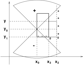
Figure 2:

First we construct the rectangle on the right hand side. (See Fig. 2.) If (i) holds in Lemma 14 for the point $(x_{0},y_{0})$ and for $x_{2}$ then we are done, so as the other two cases are similar we assume that (ii) holds. This means that even for the maximum $y_{1}$ of the zero set of $H$ between the two sectors on this vertical line, $y_{1}<y_{0}$ holds. We choose the leftmost point $(x_{3},y_{1})$ of the zero set on the segment $[x_{0},x_{2}]\times\{y_{1}\}$ as the lower right corner of the rectangle and we choose the upper right corner from the upper sector. Clearly there are only negative values on the bottom edge, so what remains to show is that all values are positive above $(x_{3},y_{1})$ on the vertical line until it reaches the upper sector. If $x_{3}=x_{2}$ then we are done, otherwise this is an easy consequence of Lemma 13 once we apply it to $x_{3},x_{2},y_{1}$ and any number $y_{2}>y_{1}$ such that $(x_{3},y_{2})$ is still between the two sectors.

Figure 3:

Now we turn to the left hand side. (See Fig. 3.) We assume again that (ii) of Lemma 14 holds for $x_{1}$, and choose a maximal $y_{3}$ such that $(x_{1},y_{3})$ is between the two sectors and $h(x_{1},y_{3})=0$. Note that, by (ii), we have $y_{3}<y_{0}$. Let $(x_{4},y_{3})$ be the rightmost point of the zero set of $H$ on the segment $[x_{1},x_{0}]\times\{y_{3}\}$. Let us now define the lower left corner $(x_{4},y_{4})$ of the rectangle as the point of maximal $y$ coordinate on the vertical line $x=x_{4}$ between the sectors, where $H$ vanishes. By Lemma 14, $y_{4}<y_{0}$ and clearly all values on the vertical half-line are positive until it reaches the upper sector. Thus we only have to show that $H(x,y_{4})<0$ for all $x_{4}<x<x_{0}$, which easily follows from Lemma 13 once we apply it to $x_{4},x,y_{3}$ and $y_{4}$. ∎

Remark 2.

Theorem 7 is not true for every $\mathbb{R}^{2}\to\mathbb{R}$ differentiable function with nowhere vanishing gradient. For an example see [2].

References

- [1] A. Bruckner, Differentiation of Real Functions, CRM Monograph Series, 1994.
- [2] Z. Buczolich, Level sets of functions with non-vanishing gradient, Journ. Math. Anal. Appl. 185 (1994), 27-35.
- [3] M. Csörnyei, T. C. O’Neil, D. Preiss, The composition of two derivatives has a fixed point, to appear in Real Anal. Exchange.
- [4] R. Gibson, T. Natkaniec, Darboux like functions. Old problems and new results, Real Anal. Exchange 24 (2) (1998-99), 487-496.
- [5] I. Maximoff, Sur la transformation continue des fonctions Bull. Soc. Phys. Math. Kazan 12 (1940), no. 3, 9-41 (Russian, French summary).
- [6] D. Preiss, Maximoff’s Theorem, Real Anal. Exchange 5 (1) (1979-80), 92-104.
- [7] G. T. Whyburn, Analytic Topology, AMS Colloquium Publications Vol. 28, 1942.