CERN-PH-TH/2011-228
DESY 11-124
Monte Carlo tuning in the presence of Matching
B. Cooper1, J. Katzy2, M. L. Mangano3, A. Messina3,
L. Mijović2, P. Skands3
1 Department of Physics & Astronomy, University College London, WC1E 6BT, UK
2 Deutsches Electron Synchroton, 22603 Hamburg, Germany
3 European Organization for Nuclear Research, CERN CH-1211,
Geneva 23, Switzerland
We consider the impact of varying choices (and scales) on each side of the so-called “matching scale” in MLM-matched matrix-element + parton-shower predictions of collider observables. We explain how inconsistent prescriptions can lead to counter-intuitive results and present a few explicit examples, focusing mostly on + jets processes. We give a specific prescription for how to improve the consistency of the matching and also address how to perform consistent tune variations (e.g., of the renormalization scale) around a central choice. Comparisons to several collider processes are included to illustrate the properties of the resulting improved matching, relying on AlpGen + Pythia 6, with the latter using the so-called Perugia 2011 tunes, developed as part of this effort.
1 Introduction
The theoretical description of multijet production in hadronic collisions is one of the key ingredients for the interpretation of the data from high-energy hadron colliders, the 1.96 TeV proton-antiproton Tevatron collider at Fermilab, and the proton-proton Large Hadron Collider (LHC) at CERN. Final states with multijets, possibly associated with electroweak gauge bosons, are in fact the dominant signature of the decay of heavy particles produced at high energy, whether in the Standard Model (top quarks and Higgs bosons), or in theories beyond the Standard Model (BSM), such as supersymmetry. The identification of these particles, and the study of their properties, requires an accurate modelling of the Standard Model (SM) sources of multijets. Great progress was achieved towards this goal in the past decade. On one side, the calculation of inclusive, parton-level, cross-sections to next-to-leading-order (NLO) in QCD has produced results for processes as complex as W+4 jets [1]. On the other, algorithms have been developed and implemented in numerical codes to provide a complete description of the hadronic final states emerging from processes with up to 6 jets, merging the exact leading-order (LO) calculation of the partonic matrix elements (ME) with the evolution, provided by so-called shower Monte Carlo (MC) codes, of the partonic shower (PS) and the subsequent hadronization of the partons in to physical hadrons.
The development of theoretical tools has been accompanied by experimental measurements, which provide the necessary validation test-bed for these calculations. Parton-level NLO calculations provide a first-principle description of inclusive final states: they have an intrinsic high degree of precision, due to the reduced dependence on the unphysical choice of a renormalization and factorization scale and, furthermore, are not subject to modelling uncertainties related to the details of the non-perturbative phase of the final state evolution. Calculations based on the merging of LO matrix elements, shower evolution and hadronization, on the other hand, while affected by the larger scale-setting uncertainty due to the LO approximation, provide a fully exclusive description of the final states, and are therefore more suitable for the experimental analyses. Their ultimate goal is not only to give reliable estimates of the inclusive jet rates and energy distributions, but also to reproduce properties of the final states such as the jet inner structure and the distribution of softer particles produced outside of the jets, including those resulting from the evolution of the fragments of the original colliding hadrons111We refer to the ensemble of these particles as the underlying event , or UE. These properties, which depend on the details of the non-perturbative dynamics, can only be described through the phenomenological models embedded in the shower MC codes. The parameters of these phenomenological models need to be tuned using experimental data of some suitable observables. The factorization assumption built into any description of large-Q processes justifies the use of these same parameters in the prediction of different observables, and provides the basis for the predictive power of such tools. This assumption however must be validated with a direct comparison with data. Elements that need to be probed include the scaling with beam energy of the UE parameters, the universality of the parameters controlling the shower evolution and hadronization, and the overall independence of all parameters on the type of hard process. Deviations from the expected universality would highlight faults in the underlying modelling of effects beyond perturbative physics, or could be due to the insufficient precision of the perturbative description, in case NLO effects were to modify significantly the LO predictions. Differences compatible with the theoretical systematics of the LO approximation could however be reabsorbed by modifying the perturbative parameters that govern the LO systematics, for example the renormalization and factorization scales, or the matching variables used in the matrix-element/shower merging algorithm.
It is therefore important to understand the correlations between the effects of changing the soft and UE parameters on one side, and the perturbative parameters on the other. In this paper we present studies which demonstrate that, in the tuning of ME-PS matched predictions, it is vital that there is consistency in the treatment of in both the ME and PS components. While this is a general issue for all shower MCs, we consider as an explicit example the merging of LO matrix elements with the Pythia 6 shower MC [2], as implemented in the framework of the AlpGen code [3], one of the reference tools for experimental multijet studies at the Tevatron and at the LHC. The most recent versions of Pythia (6.425) and AlpGen (2.14) codes were used for producing the results.
On the Pythia 6 side, we consider several different tune variations of the interleaved -ordered parton-shower model [4], focusing on the so-called “Perugia” set of tunes of [5, 6], ranging from the Perugia 0 tune (from 2009) to the Perugia 2011 updates that have been developed as part of this work, including systematic up/down variations of the shower activity (see the Appendix and [5, 6] for details). We also compare to the “DW” tune [7] of the virtuality-ordered shower model [8, 9]. For Herwig [10], we include the “Jimmy” underlying-event model [11], with default parameters. We emphasize that the qualitative conclusions presented in this paper carry over to other shower models, including the ones implemented in Pythia 8 [12, 13] and Herwig ++ [14], but the quantitative aspects should still be considered limited to the particular tunes and shower models studied here. We rely on Fastjet [15] for jet clustering and have further used the Rivet-based [16] mcplots web site [17] for some of our comparisons.
The paper is organised as follows: in Section 2 we describe in detail the theoretical nature of the consistency problem, and give a practical example of how it can be manifest in the prediction of high observables. In Section 3 we show how a simple prescription can be applied to stabilise ME-PS tunings against this problem, propose a new tune for AlpGen + Pythia 6 matched predictions, and demonstrate the behaviour of this tune under tuning variations. In Section 4 we show that this new AlpGen + Pythia 6 tune is able to reproduce (within statistical errors) the Tevatron and LHC vector boson plus jets data. In addition we also the tune predictions to the jet shape measurements at the Tevatron and LHC. Finally we conclude in Section 5.
2 The Importance of Consistent Treatment in ME-PS Matched Predictions
In this section we demonstrate that consistent treatment of in ME-PS matched predictions is important in order to achieve the desired accuracy in the prediction of high observables. We first present the theoretical arguments behind this, and then go on to show and explain that without adopting this approach one can observe undesirable and counter-intuitive effects on experimental observables.
2.1 Theoretical Background
The philosophy behind matching prescriptions such as the MLM one [18, 19] employed by AlpGen is to separate phase space cleanly into two distinct regions; a short-distance one, which is supposed to be described by matrix elements, and a long-distance one described by parton showers. In the long-distance region, real and virtual corrections, with the latter represented by Sudakov factors, are both generated by the shower and are intimately related by unitarity (for pedagogical reviews, see, e.g., [20, 21]). On the short-distance side, the real corrections are generated by the matrix elements while the virtual ones are still generated by the shower.
Much effort has gone into ensuring that the behaviour across the boundary between the two regions be as smooth as possible. CKKW showed [22] that it is possible to remove any dependence on this “matching scale” at NLL precision by careful choices of all ingredients in the matching; technical details of the implementation are important, and the dependence on the unphysical matching scale may be larger than NLL unless the implementation matches the theoretical algorithm precisely [23, 24, 25].
Especially when two different computer codes are used for matrix elements and showering, respectively (as when AlpGen or MadGraph [26] is combined with Pythia 6 or Herwig), inconsistent parameter sets between the two codes can jeopardise the consistency of the calculation and lead to unexpected results, as will be illustrated in the following sections.
To give a very simple theoretical example, suppose a matched matrix-element generator (MG) uses a different definition of than the parton-shower generator (SG). Suppressing parton luminosity factors to avoid clutter, the real corrections, integrated over the hard part of phase space, for some arbitrary final state , will then have the form
| (1) |
where we have factored out the coupling corresponding to the “+1” parton and suppressed the dependence on any other couplings that may be present in . The virtual corrections at the same order, generated by the shower off , will have the form
| (2) |
with the DGLAP splitting kernels (or equivalent radiation functions in dipole or antenna shower approaches). If the two codes use the same definitions for the strong coupling, , then the fact that captures the leading singularities of guarantees that the difference between the two expressions can at most be a non-singular term. Integrated over phase space, such a term merely leads to a finite change to the total cross section, which is within the expected precision. Indeed, it is a central ingredient in both the MLM and (L)-CKKW matching prescriptions that a reweighting of the matched matrix elements be performed in order to ensure that the scales appearing in match smoothly between the hard and soft regions. Thus, we may assume that the choice of renormalization scale after matching is on both sides of the matching scale, where is a scale characterising the momentum transfer at each emission vertex, as established by [27, 28] and encoded in the CKKW formalism [22].
In the case of the CKKW approach as implemented in the Sherpa MC framework [29], this prescription can be controlled exactly, since the matrix element and the shower evolution are part of the same computer code and hence naturally use the same definition. This is also true in Lönnblad’s variant [23] of the algorithm, used in Ariadne [30]. In the case of codes like AlpGen or Madgraph, on the other hand, an issue emerges. These codes are designed to generate parton-level event samples to be used with an arbitrary shower MC. Different shower MCs however use slightly different scales for the parton branchings, as a result of different approaches to the shower evolution, and may use different values of , as a result of the tuning of the showers and/or underlying events. A possible mismatch therefore arises in the values of used by the matrix-element calculation and those used by the shower.
If there is a mismatch in or , then this will effectively generate a real-virtual difference whose leading singularities are proportional to
| (3) |
which is of next-to-leading logarithmic order (unless , in which case it vanishes). Similarly, even if both matrix-element and shower codes are using the same , but they use different running orders, then there will be an mismatch, which may also become large if .
To be more concrete, let us consider a specific example. Compare A) a matched MG+SG calculation which uses the same value on both sides of the matching to B) a calculation in which the value used on the MG side is reduced to half its previous value but the SG one remains the same, as summarised by the two first columns of tab. 1.
| A | B | C | |
|---|---|---|---|
Going from case A to B, the following changes result:
-
1.
The number of states added by the MG decreases, due to the lowering of the value on the MG side, while the number of surviving states remains constant, since the shower Sudakov is not modified. The total estimated cross section therefore decreases.
-
2.
At the differential level, the smaller number of states combined with the unchanging number of states implies smaller absolute jet cross sections and smaller fractions .
Similarly we may consider what happens if C) we reduce the value on the SG side instead, as summarised in the last column of tab. 1. Going from case A to C, the following changes result:
-
1.
The number of states added by the MG remains constant, while the number of surviving states increases, since the SG is generating fewer branchings. The total estimated cross section therefore increases.
-
2.
Since the number of states is constant, while the shower is made less active, the final jets will actually be narrower, which increases the rate of reconstructed jets at any given fixed value.
-
3.
Since both the total cross section increases and the number of reconstructed additional jets also increases, jet fractions can either increase or decrease.
In particular, note the somewhat counter-intuitive effect that decreasing the shower value actually increases the jet rates in a matched calculation, while it normally decreases them in a standalone shower calculation.
Since, as was discussed above, inconsistencies among the choices on the two sides can lead to differences at the NLL level, it is obviously important to ensure that they are consistent within a reasonable margin. This is particularly true in the context of event-generator tuning, in which specifically the NLL components of the shower description are sought to be optimized with respect to measured data, and hence changes at this level could effectively destroy the tuning.
Finally, we remind the reader that a change in can be interpreted as a change in the opposite direction of the renormalization scale argument (for constant ), modulo small flavour threshold effects that we shall ignore here. This is easy to realise from the definition of the coupling,
| (4) |
Thus, we may write renormalization scale variations (e.g., by a factor of 2 in each direction) either by applying a prefactor directly on the renormalization scale argument of or by applying the inverse of that factor to while keeping the renormalization scale argument unchanged. Due to the technical structure of the codes, the former is more convenient in AlpGen (via the ktfac setting) whilst the latter is more convenient for Pythia 6.
2.2 Examples of the interplay between tunes and matching
In this section we give several examples of how the issues in ME-PS matching described in Section 2 can affect high- observables using AlpGen interfaced to Pythia 6 with DW [7], Perugia 0 (P0) [5, 31] and Perugia 2010 (P2010) tunes [6].
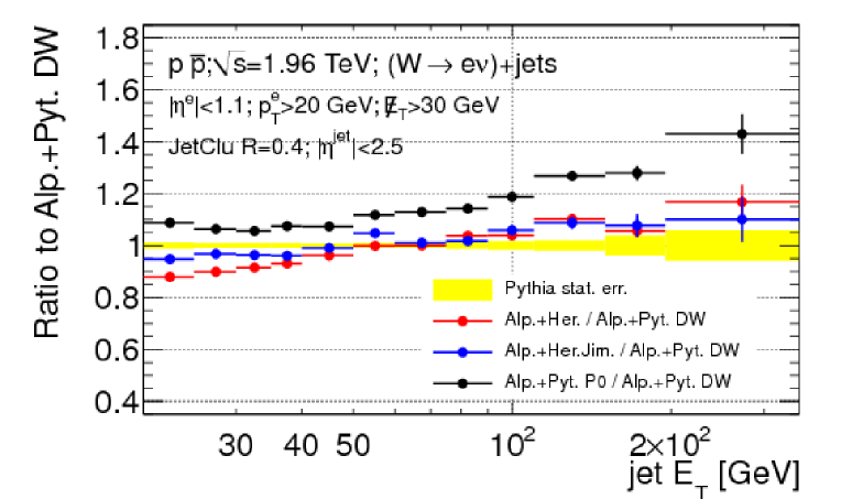
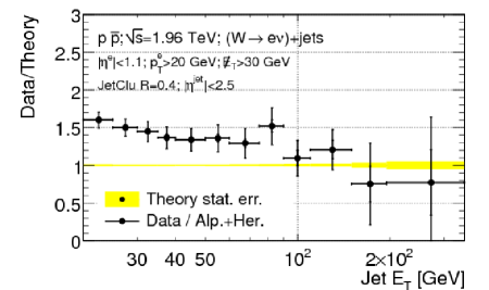
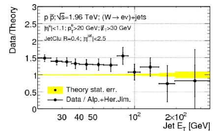
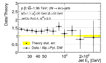
In Fig. 1 we show the ratio of predictions for the transverse energy () spectrum of the leading jet (that jet with the highest per event) in +jet final states at the Tevatron, obtained by the merging of AlpGen with different shower codes; Herwig, Pythia 6 virtuality-ordered shower (DW), and -ordered shower (Perugia 0). The differences between Herwig and Herwig plus Jimmy at small can be explained by the different amounts of energy that, in the various cases, are deposited by the UE in the jet cones. In particular, as shown in Fig. 2, these differences can accommodate the slight shape discrepancy between data and AlpGen +Herwig that was noted, at small , in the CDF study [32]. It is difficult, however, to attribute to the UE energy the significant differences seen in Fig. 1 at large .
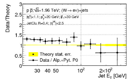
In order to investigate the source of the differences in the predictions, systematic parameter variations of the perturbative and non-perturbative model components of Pythia 6 have been studied using the Perugia family of Pythia 6 tunes with Perugia 0 as the central tune and Perugia Hard and Perugia Soft as the systematic variation tunes. The Perugia Soft and Perugia Hard tunes both use the same Parton Density Function (PDF) as Perugia 0, CTEQ5L [33], but differ in the values of Pythia 6 parameters controlling both perturbative and non-perturbative activity levels. In comparison to Perugia Soft, the Perugia Hard tune has more perturbative (initial and final state radiation) activity but less non-perturbative (multiple interactions, beam remnant and hadronization) activity. Perugia Soft on the other hand has less perturbative but more non-perturbative activity than the Perugia 0 tune. In order to investigate the interplay of the tuning variations with the MLM matching, the effect of the change of the tune on the physics observables in both the Pythia 6 standalone case and AlpGen + Pythia 6 case is presented.
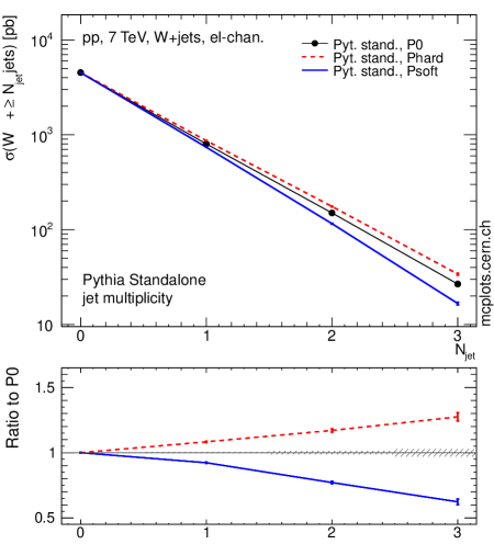
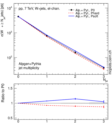
In Fig. 3 the distribution of jet multiplicity () in +jets events is compared for events generated with the Perugia 0, Perugia Hard and Perugia Soft tunes. The observable is defined at the particle-level according to the definition used in the ATLAS measurement of the +jets cross-section at =7 TeV [34]. Jets are clustered from stable particles using the anti-Kt jet algorithm [35] with the radius parameter , and considered in case they satisfy the following kinematic cuts: and . Comparisons are performed for both the Pythia 6 standalone (left) and AlpGen + Pythia 6 (right) cases. For the Pythia 6 standalone case we observe that Perugia Hard tune yields more high- jets than the Perugia 0 tune while Perugia Soft yields less final state jets correspondingly. For the AlpGen + Pythia 6 case an opposite trend is observed: Perugia Hard tune yields less high- jets and Perugia Soft tune yields more high- jets. In order to determine which modelling components of the Perugia Soft and Perugia Hard tunes cause this behaviour, we considered the effect of varying individual sets of parameters of the Perugia Soft and Perugia Hard tunes in AlpGen + Pythia 6 predictions. Parameters were grouped according to the modelling aspect they control into Initial State Radiation (ISR), Final State Radiation including the FSR from the ISR partons (FISR), the Underlying Event (UE) and Colour Reconnections (CR) blocks222The parameter blocks organisation is similar to the one introduced in [6] and are listed in A.2
Dedicated samples where only parameters of an individual block were varied in the ranges used in Perugia Soft and Perugia Hard tunes on top of the Perugia 0 tune were produced. The results of the study, in terms of the cross-section contribution of each AlpGen sub-sample (after MLM matching), are given in Table 2. As was already noted in Fig. 3, the cross-section for multijet production in the Perugia Hard case decreases with respect to Perugia 0, and vice versa for Perugia Soft. From Table 2, we see that the parameter blocks that produce this affect are the ISR and FISR blocks, while the impact of the CR and UE block variations on the cross-sections is negligible. In addition to the simultaneous variations of parameters in the blocks, we have also performed individual parameter variations for each of the parameters in order to check that potential correlations between the parameters do not affect the conclusions. Studies have also been performed for the Hadronization and Beam Remnant blocks of [6]. The variations of these parameters also had a negligible effect on the kinematic distributions and cross-section values.
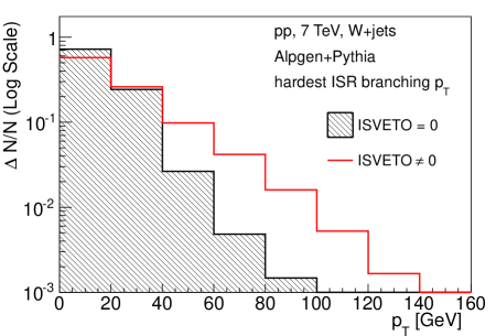
In Fig. 4 we demonstrate that the increased parton shower activity can indeed lead to the reduced cross-section (and softer jet spectra) due to the increased rates at which the AlpGen + Pythia 6 events are vetoed during the MLM matching. In the figure the distributions of the events that pass or fail (ISVETO=0 or ISVETO0) the MLM matching criterion are shown for the exclusive sub-sample of AlpGen + Pythia 6 Perugia 2010 +jets events with exactly three additional partons from the matrix element in the final state333The observations in the text are largely independent on the final state parton multiplicity. Each of the distributions is normalised to unit area. The distributions are shown as a function of the largest shower emission from the initial state radiation (left) and as a function of the largest multiple proton-proton interaction. 444These values are reported by Pythia 6 parameters VINT(357) (ISR) and VINT(359) (MPI) respectively. In the left hand side figure we see that the events are rejected with higher probability, the larger the of the hardest ISR branching in the event. Therefore, a Pythia 6 standalone tune which increases the ISR activity can, somewhat counter-intuitively, reduce the rate for multijet and hard emissions. In the right hand side we demonstrate that the events are accepted and rejected independently of the transverse momentum of the hardest multiple interaction in the event (which is the desired behaviour of the matching application used with the parton shower code).
| tune | Np0 | Np1 | Np2 | Np3 | Np4+ | total [pb] |
|---|---|---|---|---|---|---|
| Phard | 7287 3.9 | 728 2.6 | 141 1.3 | 27 0.2 | 6.6 0.2 | 8190 8 |
| P0 | 7556 3.6 | 814 2.7 | 166 1.3 | 32 0.3 | 7.8 0.3 | 8576 8 |
| Psoft | 7804 3.4 | 944 2.8 | 207 1.5 | 42 0.3 | 10.1 0.3 | 9007 8 |
| P0 with Phard ISR | 7207 6.9 | 735 2.6 | 143 1.3 | 27 0.2 | 6.9 0.2 | 8119 11 |
| P0 with Psoft ISR | 7831 4.9 | 881 2.7 | 186 1.4 | 36 0.3 | 8.8 0.3 | 8943 10 |
| P0 with Phard FISR | 7548 6.0 | 814 2.7 | 167 1.3 | 32 0.3 | 7.8 0.3 | 8569 10 |
| P0 with Psoft FISR | 7505 6.1 | 878 2.7 | 188 1.4 | 37 0.3 | 9.4 0.3 | 8617 10 |
| P0 with Phard UE | 7513 6.1 | 826 2.7 | 171 1.4 | 33 0.3 | 7.8 0.3 | 8551 10 |
| P0 with Psoft UE | 7576 5.9 | 817 2.7 | 166 1.3 | 32 0.3 | 8.1 0.3 | 8599 10 |
| P0 with Phard CR | 7561 5.9 | 821 2.7 | 167 1.3 | 32 0.3 | 8.1 0.3 | 8589 10 |
| P0 with Psoft CR | 7556 5.9 | 815 2.7 | 165 1.3 | 32 0.3 | 8.1 0.3 | 8576 10 |
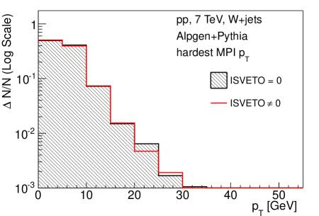
To conclude, the origin of the differences observed in the predictions of tunes with different ISR/FSR activity matched to AlpGen is rather due to the mismatch between the jet-emission probability predicted by the matrix elements and by the shower. This comes from the mismatch in the value of discussed earlier, arising from different values of or from the use of a different evolution variable in the shower. If the value of in the shower increases, the emission rate of additional jets during the shower evolution will increase. Since the matching algorithm rejects events with extra jets generated by the shower, to replace them with events where the jet is accounted for by a higher-order matrix element calculation, a larger value of in the shower leads to a higher rejection rate. Unless this change in is accompanied by a similar change in the matrix element calculation, the additional rejection is not compensated by the relative increase in rate for the higher-order parton-level contributions, leading to the effects reported in this section.
This important interplay between MC parameters, which are typically tuned to “soft” observables such as UE or the small- DY spectrum, and the performance of the matching algorithms for “hard” observables, calls for particular attention when adopting new UE tunes in the framework of multijet studies with matrix-element matching. Along the same lines, it should be kept in mind that, tuning a stand-alone shower MC to better model multijet final states, will force it to emulate effects present in the multiparton matrix elements. Using such tunes with matrix-element matching therefore requires ad-hoc modifications of the matching algorithm, or of its parameters.
3 Stabilising ME-PS Matched Tunings
In this section we discuss how to overcome the problems discussed in the previous section with a simple prescription, and outline a tuning strategy that should allow to consistently optimize, in the context of the Pythia 6 shower MC, the description of both the UE and the high- properties of final states.
3.1 A New AlpGen + Pythia 6 Consistent Tune
As it was explained in Section 2.1, and practically demonstrated in Section 2.2, it is highly desirable to have a consistent treatment of on either side of the ME and PS boundary. In Appendix A.1 the relevant settings for a new consistent AlpGen + Pythia 6 tune are described in detail. In this tune, the consistency is essentially ensured by setting the effective value of to be the same throughout the Pythia 6 parton shower algorithms and in the AlpGen matrix elements. A consistent choice for of
| (5) |
is made, where the superscript indicates the number of flavours. This choice is informed by comprehensive Professor tunings [36, 37] of the -ordered shower in Pythia 6 [4] to event shapes and other LEP data. Note that the settings for Pythia 6 are those of the central Perugia 2011 (P2011) tune [6], which was inspired by these studies. We will refer to this new tune of AlpGen + Pythia 6 as the Perugia 2011 “matched” tune.
3.2 Tests of the Consistent Approach: Behaviour Under Scale Variations
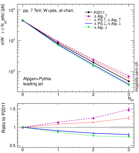
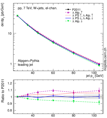
In this section we study the behaviour of the new AlpGen + Pythia 6 Perugia 2011 “matched” tune under variations to demonstrate that, with a consistent treatment of , the expected behaviour of ME-PS matched predictions under variations of tuning parameters is restored. +jets events selected with the same criteria applied for Fig. 3 are used. Figure 5 shows the jet multiplicity (left) and leading jet transverse momentum (right) distributions for the Perugia 2011 “matched” tune and four variant tune samples generated with different values. Two samples, labelled as “” and “”, have respectively increased and decreased by a factor of 2 only in the ME calculation. This is achieved by setting respectively the AlpGen parameter ktfac to 1/2 and 2. The increase (decrease) of the value in AlpGen results in more (less) jets and a harder (softer) leading jet spectrum as shown in Fig. 5. The two samples labelled as “” and “” correspond to a consistent variation of both in the ME and PS, with respectively increased and decreased by a factor of 2. The impact of these variations is qualitatively similar to the case where is only varied in the ME, restoring the expected behaviour of ME-PS matched prediction under variation of . However, the samples with varied simultaneously in the ME and in the PS exhibit a smaller deviation from the nominal sample. The mitigation of the impact of a coherent change in a ME-PS matched sample compared to the same change only in the ME calculation is due to the interplay between the radiation produced by PS and the matching algorithm, as detailed in Section 2.1. While the choice of the xlclu parameter allows to directly adapt AlpGen to possible future changes in the choice of in Pythia, the variation of the ktfac parameter in the standard range can be used to establish the range of the systematical uncertainty, or to tune the description of specific observables.
4 Comparisons with Data
In this section we demonstrate that the new -consistent Perugia 2011 “matched” tuning of AlpGen + Pythia 6 introduced in Section 3.1 compares well with recent Tevatron and LHC measurements, and that, with the arrival of improved precision measurements, there should be room for further tuning of these predictions.
4.1 /+jets production
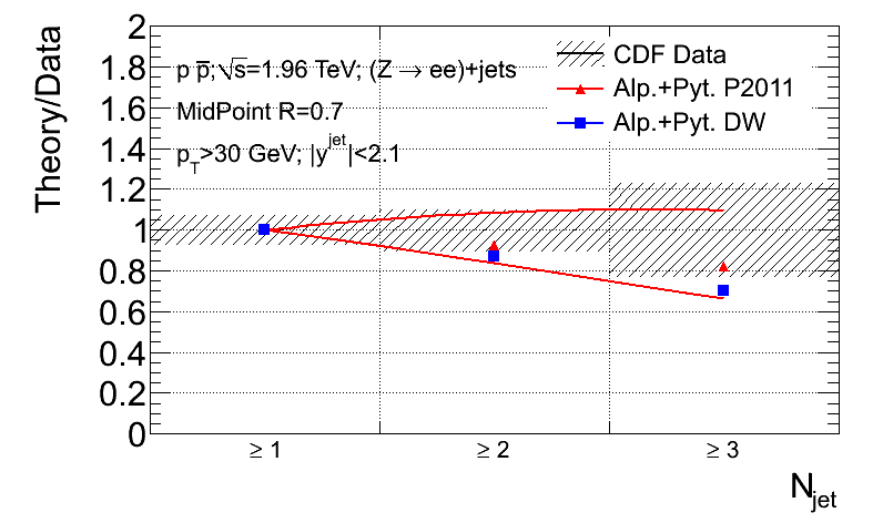
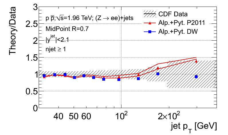
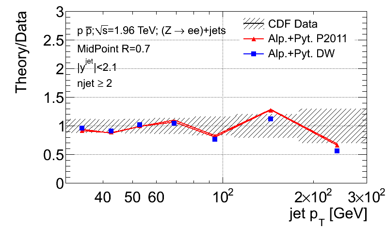
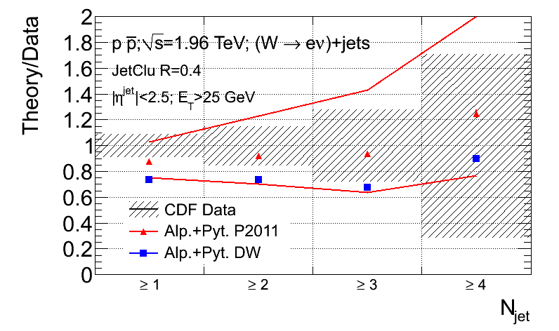
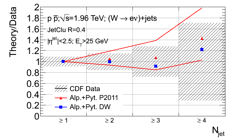
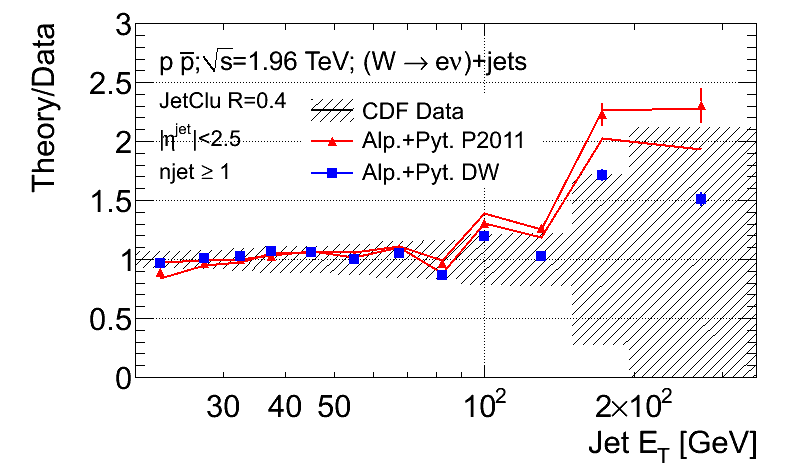
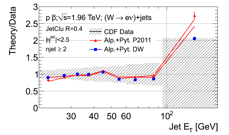
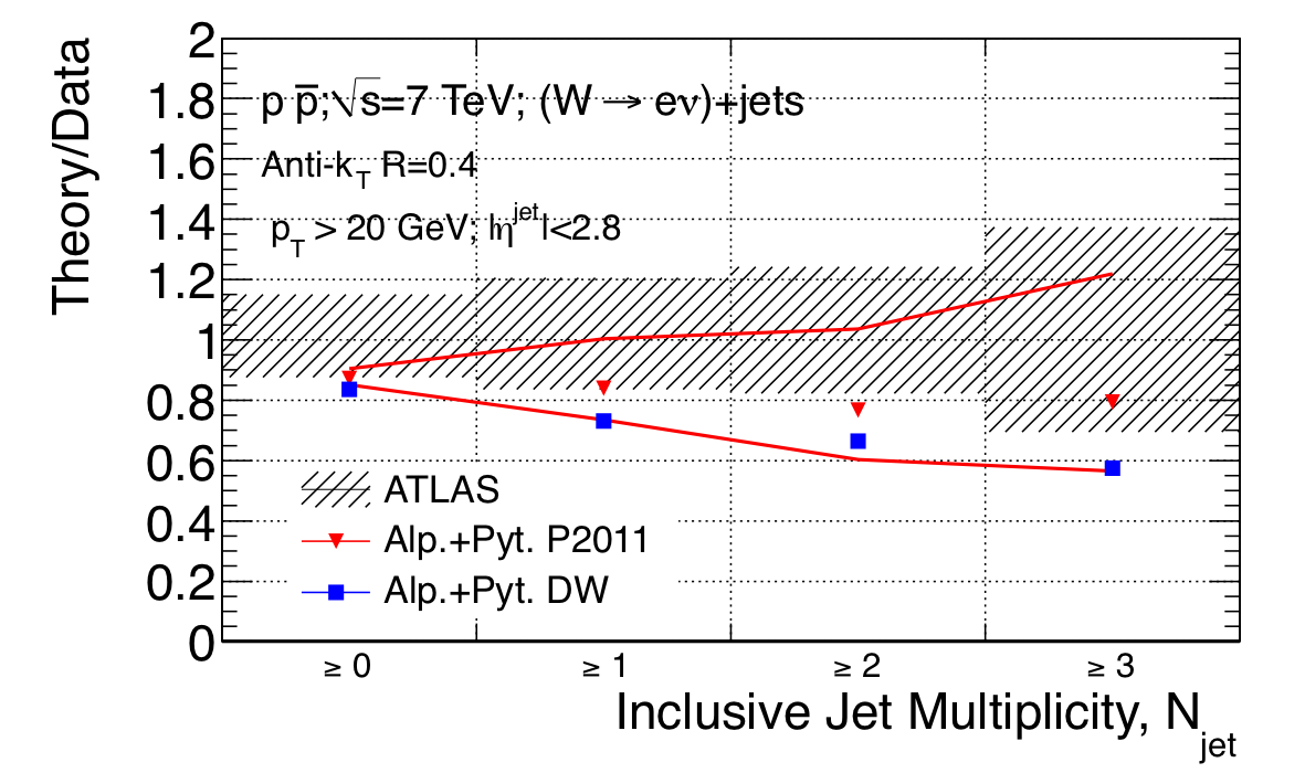
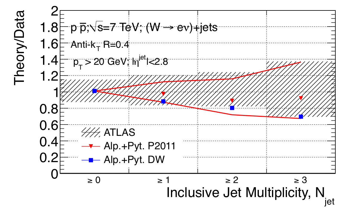
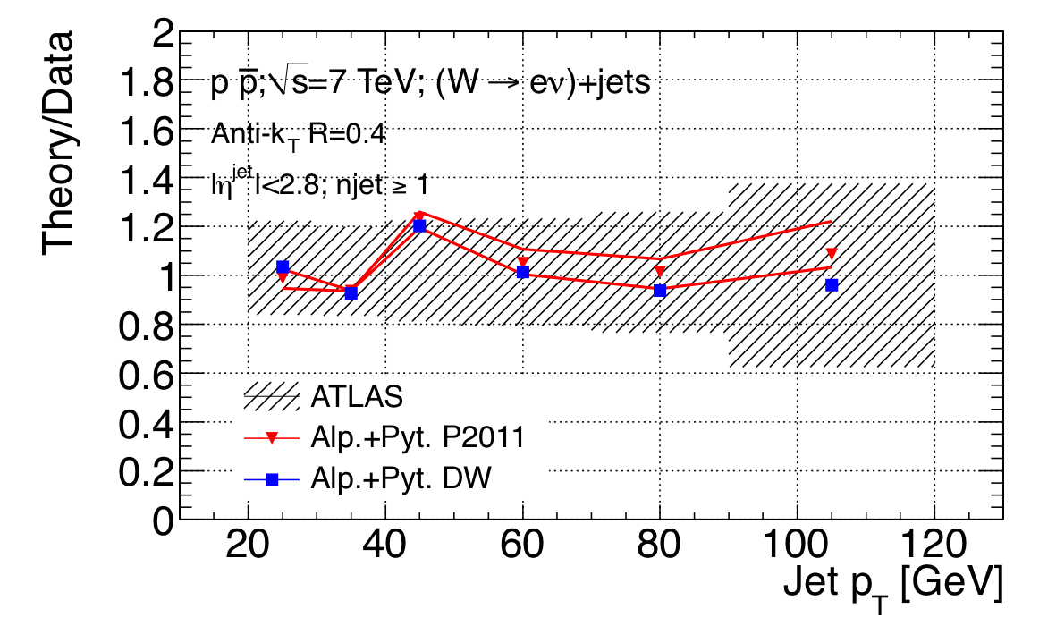
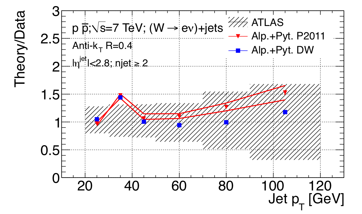
The figures that follow show comparisons of AlpGen + Pythia 6 Monte Carlo predictions to measurements of published +jets and +jets processes from CDF [38, 32, 39] and +jets from ATLAS [40]555Measurements of these processes at the Tevatron have also been performed by D0 [41, 42, 43]. Preliminary, higher statistics, studies of +jets production at the LHC have been reported by ATLAS [34, 44], and CMS [45].. These cross-section measurements are corrected for all known detector effects to particle level and compared to Monte Carlo predictions. The Monte Carlo predictions of +jet production cross-sections are formed by clustering the stable final state particles ( ps) following parton shower and hadronization of the unweighted events. This clustering is done using the same jet algorithm as the measurement, as implemented in the Fastjet [15] package. All stable final state particles are used, with the exception of the leptons that result from the decay of the signal or boson. The decay leptons are corrected for the final state QED radiation such that their 4-momentum is equivalent to that before radiation. After the events have been clustered, the restrictions on the allowed phase space of the jets and of the / boson decay products are applied to be consistent with the measurement to which we are comparing. The prediction of the final AlpGen + Pythia 6 cross-sections contains contributions from +0, 1, 2, 3 parton samples (showered with exclusive MLM matching), and +4 parton samples (showered with inclusive MLM matching).
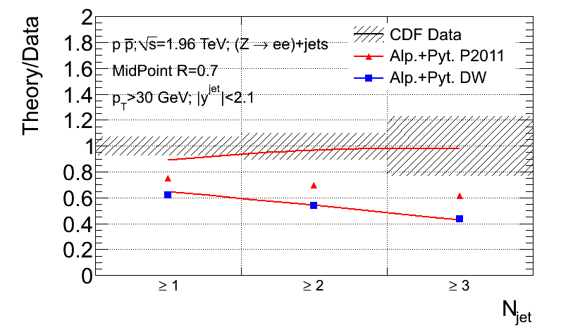
Two different AlpGen + Pythia 6 generations are compared to the data; the new AlpGen + Pythia 6 Perugia 2011 “matched” tune introduced in Section 3.1 (labelled “Alp.+Pyt. P2011”), and an AlpGen + Pythia 6 prediction using the default settings of AlpGen and the Pythia 6 DW tune (labelled “Alp.+Pyt. DW”). The ratio of the matched predictions to the data are shown and compared. Additionally, the results of variations of ktfac by factors of 0.5 and 2.0 in the AlpGen + Pythia 6 Perugia 2011 “matched” prediction are shown as solid lines. The hatched regions show the total error (statistical plus systematic) propagated to the theory/data ratio from the data measurements. The error bars on the points show the statistical error on the theoretical prediction.
In Figure 6 we show the ratio of the predicted theory cross-sections to the data for the CDF +jets measurement [39]. In this measurement jets are defined by the CDF midpoint algorithm [46], with and are required to have and . In Figure 7 we show the ratio of the predicted theory cross-sections to the data for the CDF +jets measurement [32]. In this measurement jets are defined by the CDF JetClu algorithm [47], with and are required to have and . In Figure 8 we show the ratio of the predicted theory cross-sections to the data for the ATLAS +jets measurements [40]. In this measurement jets are defined by the anti-Kt algorithm [35], with a radius parameter and are required to have and .
The AlpGen + Pythia 6 Perugia 2011 “matched” prediction compares well with the measured cross sections both as a function of the inclusive jet multiplicity and jet . In particular, the prediction correctly describes the low region of the differential cross section and the jet sub-structure without presenting any significant disagreement with data at high . This shows that it is possible to tune separately the long- and short-distance contributions of the prediction to obtain a satisfactory description of the observables in the whole experimental accessible phase space. Remarkably, the prediction describes the data both at TeV and TeV. This illustrates that the scaling properties of the long-distance contribution with the centre of mass energy of the collision does not produce unexpected effects in the high region of the cross section. A coherent rescaling of with ktfac =0.5, 2 has a little effect on the shapes of the differential cross-sections, while for the inclusive cross-sections it produces variations that bracket the default prediction. The ktfac parameter can therefore be used to explore the sensitivity of the prediction to a variation of the renormalization and factorization scale, other than allow tuning on data. With the statistics of the currently available measurements there is no much room for optimising the parameters of the AlpGen + Pythia 6 Perugia 2011 “matched” prediction in a tune that better describes the measurements. However, with the imminent arrival of more precise higher-statistics LHC measurements, this should be possible in the near future.
Even though not explicitly shown here, in the relevant publications one can find similarly good agreement between the available measurements [32, 34, 44] and predictions based on AlpGen + Herwig.
4.2 Jets shapes
Finally we test the ability of the new AlpGen + Pythia 6 Perugia 2011 “matched” tune and the systematics variations to describe the jet shapes at the LHC and the Tevatron.
For the LHC, the jet shapes measured in inclusive jet production by the ATLAS collaboration [48] are taken as reference. For this measurement the jets are reconstructed using the anti-kt algorithm with the distance parameter =0.6, the transverse momentum range 30 GeV 600 GeV and rapidity in the region 2.8. The jet shapes are expected to be sensitive to both perturbative (parton shower) and non-perturbative (fragmentation and underlying event) modelling aspects. We perform the data comparisons for both the AlpGen + Pythia 6 and Pythia 6 standalone cases. The samples are generated using different Pythia 6 standalone and AlpGen + Pythia 6 parameter settings as follows: for Pythia 6 standalone the Perugia 2011 and the associated systematics tunes Perugia 2011 radHi and Perugia 2011 radLo are compared. The same tunes are also used for the generating the AlpGen + Pythia 6 distributions whereby the values are always set to the same values in AlpGen (using ktfac) and Pythia 6 (i.e. the Perugia 2011 “matched” central settings and the systematic variations around the central settings). The setups are compared to the integral jet shape distributions as measured in the data. The integral jet shape is defined as the average fraction of the jet that lies inside a cone of radius concentric with the jet cone [48]:
| (6) |
The sum is performed over all the jets in the kinematic region of interest.
In Figure 9 the integral jet shape distributions are compared to the ATLAS data for the jets in the transverse momentum ranges of 40-60 GeV (top) and 260-310 GeV (bottom) in the whole measured rapidity range ( 2.8). We observe that both Pythia 6 standalone (left) and AlpGen + Pythia 6 (right) with Perugia 2011 provide reasonably good description of the jet shapes. Due to MLM matching the jets in the AlpGen + Pythia 6 case tend to be more narrow than in the Pythia 6 standalone case.
For the Tevatron, the shapes of jets produced in association with a Z boson as measured by CDF [49] are used. In this measurement jets are defined by the CDF midpoint algorithm [46], with and are required to have and . Figure 10 shows good agreement between AlpGen + Pythia 6 and the measurement for both the DW and Perugia 2011 tunes.
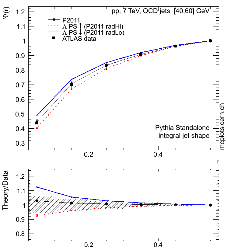
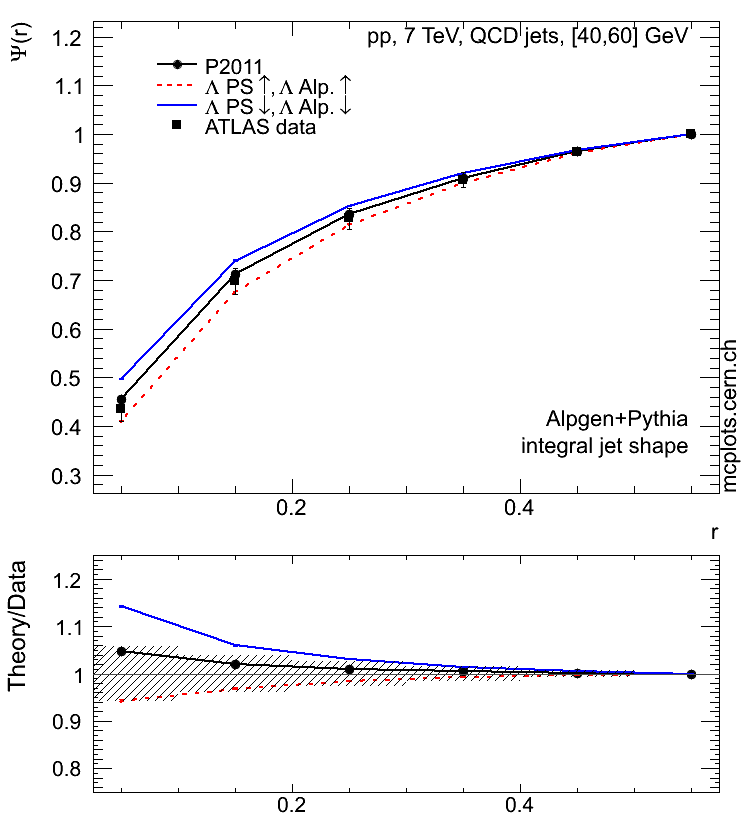
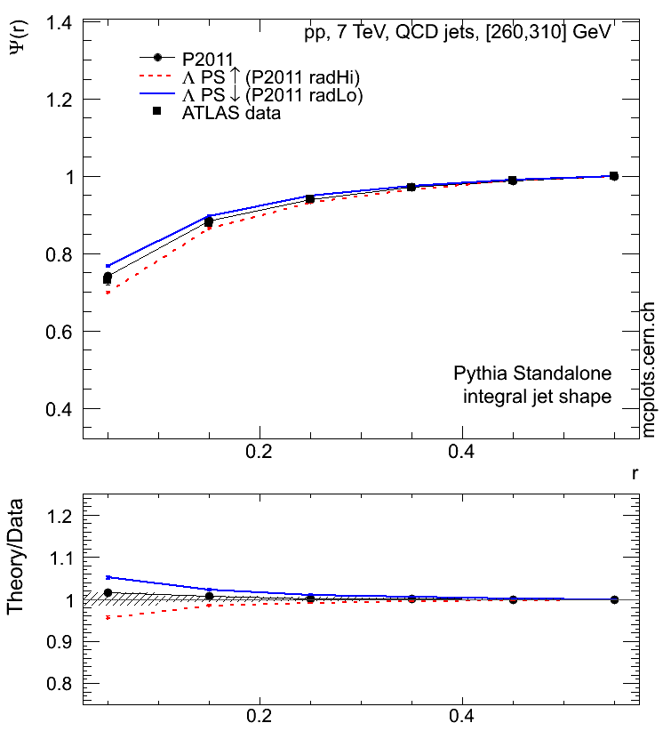
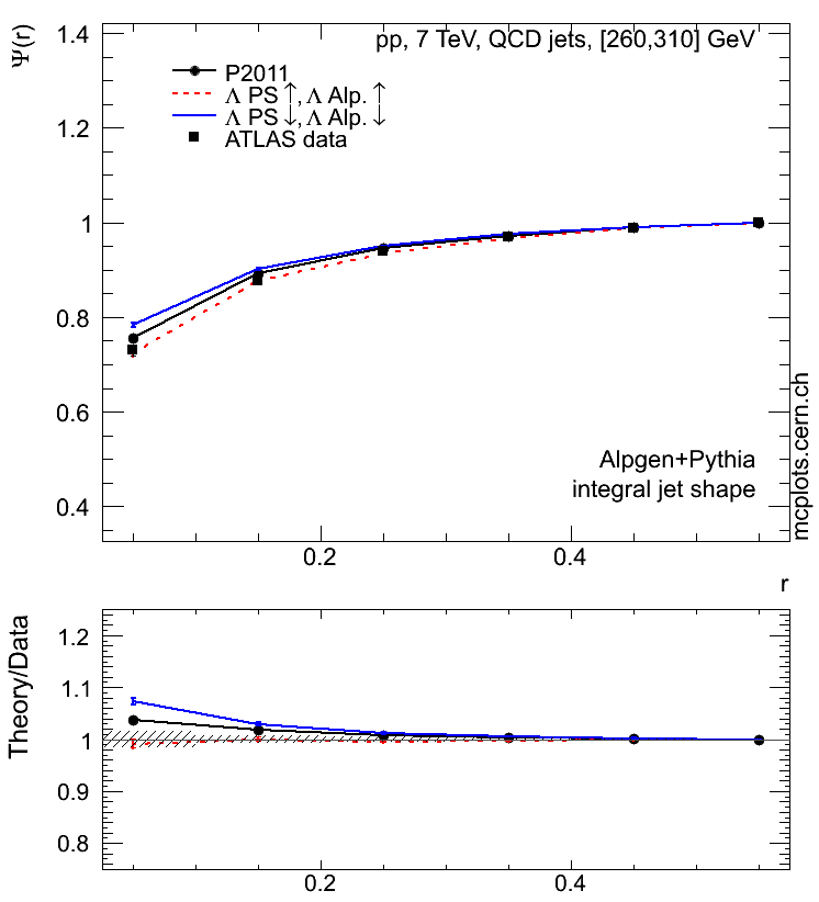
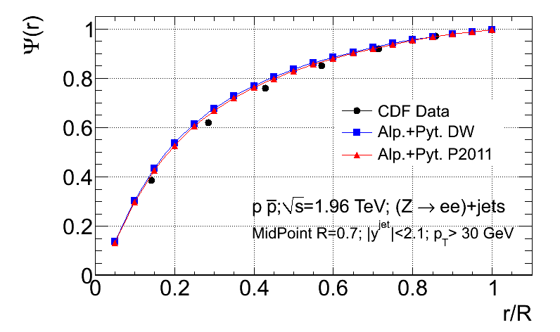
The comparisons in Figures 9 and 10 (as well as comparisons to the jet shapes in other kinematic regions and comparisons to further LHC measurements) reveal no major short-comings of the AlpGen + Pythia 6 Perugia 2011 “matched” tune. The Perugia 2011 tune has been developed by tuning Pythia 6 standalone, whereby the effective value of was set to be the same throughout the Pythia 6 parton shower in the anticipation of using it with the AlpGen matrix elements using the same effective value. The agreement with the measured jet shapes data could therefore potentially be improved by performing a dedicated tuning of AlpGen + Pythia 6.
5 Conclusions
We have shown that, in the context of tuning ME-PS matched predictions, it is vital that the tuning adopted ensures a consistent treatment of on either side of the “matching boundary”. In the case of AlpGen + Pythia 6 matched predictions, we have outlined a simple prescription to ensure this. This can be easily generalised, and applied to the case of matching AlpGen with other shower MCs, such as Herwig. We have then given an example of such a tune that compares well to Tevatron and LHC measurements of vector boson plus multijet final states. In addition, we have shown how consistent variations around a central ME-PS matched tune can be performed, so as to define a systematic uncertainty on that prediction. This knowledge should prove valuable in defining a new set of consistent ME-PS tunes for the precise future study of LHC multijet final states.
Acknowledgements
J. K. and L. M. acknowledge the support of the Initiative and Networking Fund of the Helmholtz Association, contract HA-101 (”Physics at the Terascale”). B. C. acknowledges the support of the UK Science and Technology Facilities Council (STFC). L. M. acknowledges the LPCC for the hospitality during the initial phase of this project.
Appendix A Appendix
A.1 An Consistent AlpGen + Pythia 6 Tune
We here describe the parameters in the AlpGen and Pythia 6 codes that are important for ensuring the consistency of matching, and give the settings of these parameters which describe a new consistent AlpGen + Pythia 6 tune. Note that the settings for Pythia are those of the central Perugia-2011 tune [6], which was inspired by these studies.
A.1.1 AlpGen Parameters
For AlpGen, the relevant parameters controlling the magnitude, renormalization scale, and running order for are set to these values:666The parameters xlclu and lpclu were introduced in connection with this work, and are implemented in AlpGen starting from v2.14. The default behaviour, if these parameters are not set, is to assign the values inherited from the PDF (as was the case for AlpGen versions before 2.14). :
-
•
The prefactor rescaling the value of the renormalization scale in the CKKW scale-setting procedure: ktfac = 1.0
-
•
(5-flavour): xlclu =0.26
-
•
Running order: lpclu = 1
A.1.2 Pythia Parameters
To the extent that the explanations given here are necessarily somewhat brief, we recommend the interested reader to follow up on the definitions of the parameters below in the program’s comprehensive manual [2].
The Strong Coupling in Pythia 6:
there are several different ways of specifying the parameters controlling . In order for the user to have explicit control of all of them, we use the option MSTP(3)=1, which allows to specify formally independent values for each of the different algorithmic components in Pythia. As a special case, we may then choose to set all those values equal, or at least set those equal that correspond to initial- and final-state radiation. These are:
-
•
PARP(61) for for ISR.
-
•
PARJ(81) for for FSR inside resonance decays.
-
•
PARP(72) for for FSR outside resonance decays (e.g., FSR off hard jets from the matrix element and/or from ISR).
The number of flavours with which to interpret must also be specified. Since a value of is hard-coded in at least one sub-algorithm of Pythia, we advise to always translate values to 5-flavour ones and, correspondingly, set the parameter MSTU(112)=5.
Further, in order to avoid that any of these values are modified by the code, we set MSTP(64)=2, and PARP(64)=1.0. The former forces the code to keep unmodified for ISR. In particular, the translation from “MSbar” to “CMW”, which is applied for MSTP(64)=3, is not performed. This is equivalent to interpreting the effective value as already being in a scheme similar to CMW. The latter, PARP(64)=1.0, sets the prefactor for the renormalization scale used for ISR equal to unity, i.e., the renormalization scale will just be . Any re-interpretation of , for instance to translate between different effective scheme definitions or to introduce multiplicative factors on the effective renormalization scale, for scale variation purposes, should then be imposed directly on the three values above. This is the prescription followed in the so-called Perugia 2011 tunes which were developed as part of this effort, with parameters as listed in [6].
Finally, one needs to settle on an effective value for . According to comprehensive Professor tunings [36, 37] of the -ordered shower in Pythia [4] to event shapes and other LEP data, one needs values of order
| (7) |
where the superscript indicates the number of flavours. We interpret this as an effective value, derived directly from data using a “Pythia scheme” that is defined numerically by Pythia’s shower algorithm. It is not necessarily directly comparable to determinations777It is probably closest to the so-called CMW scheme [28]. For completeness, a reasonable derived guess for a corresponding value would then be , since the CMW prescription yields effective values that are approximately 1.6 times larger than the one..
The Strong Coupling in Pythia 8:
Although we restrict the numerical studies in this paper to Pythia 6, for completeness we also include the case of Pythia 8 [50], for which the corresponding relevant parameters are
-
•
TimeShower:alphaSvalue,
-
•
TimeShower:alphaSorder,
-
•
SpaceShower:alphaSvalue,
-
•
SpaceShower:alphaSorder,
for final-state (timelike) and initial-state (spacelike) showers, respectively. Notice in particular that one here specifies the value of rather than that of . Similar comments about the effective scheme definition as for Pythia 6 apply.
Radiation Phase Space:
The size of the allowed phase space for radiation in the shower generator may also affect the matched result. In the -ordered shower in Pythia 6, the switch MSTP(72) controls the starting scale for final-state radiation off jets that are produced by initial-state radiation and/or are colour-connected to the beam. Naively, the FSR off such a parton should start at the scale at which it was created, which is obtained with MSTP(72)=2, the recommended option. Using the other available options is strongly discouraged, as these lead to a quite bad agreement with NLL resummations, underscored by Banfi et al in [51]. The Perugia 2011 tunes all use MSTP(72)=2.
Further, in the Perugia 2011 tunes, we start both the ISR and FSR evolutions at , with the Pythia evolution variable defined in [4] and SCALUP the scale parameter defined in the Les Houches Accord for event generators [52, 53]. Technically, this is achieved by setting PARP(71) = PARP(67) = 1.0, where the former controls the scale factor applied to the starting scale for FSR and the latter sets the one for ISR. Note that these parameters could still be varied somewhat around their central values, since the variable used by Pythia is not 100% identical to the definition that might be used to place cuts in a matrix-element generator, but we have not judged this difference essential at the current level of precision.
A.2 PYTHIA Tunes
In this work, we have used the Perugia 0, Perugia Hard, Perugia Soft, Perugia 2010, Perugia 2011, Perugia 2011 radHi, Perugia 2011 radLo [6], and the DW [7] tunes of Pythia 6.4 [2]. All use the CTEQ5L PDF set [33]. For a complete description, see the indicated references. The salient features of the tunes are as follows.
Tune DW [7] is a tune of the -ordered shower. It is based on the Tevatron “Tune A”, which had great success in describing the underlying event measured at the Tevatron. Contrary to Tune A, however, DW also included the Drell-Yan spectrum, for which Tune A predicted a far too soft spectrum. Tune DW therefore has a significantly lower renormalization scale for ISR (and thus a larger value of ), and 2 GeV of so-called “primordial ”, as compared to 1 GeV in Tune A. The energy scaling of the underlying event was based on comparisons between the underlying-event level at the Tevatron between 630 and 1800 GeV.
The Perugia tunes [6] are all tunes of the -ordered shower. Unlike DW, which was developed by tuning to the underlying event in jet events, the Perugia tunes primarily used minimum-bias data as drivers, relying on the universality of PYTHIA’s MPI modelling to extrapolate to the underlying event. In addition, a comprehensive update of the LEP fragmentation parameters was included in all tunes.
The first set, the Perugia 0 family, used LEP event shapes and fragmentation data, Tevatron minimum-bias data, and the Tevatron Drell-Yan spectrum. Again, the scaling from Tevatron data at 630 GeV was used to determine the scaling with CM energy, with some additional constraints from older UA5 data also included. A “Hard” and “Soft” variation attempted to vary the shower radiation up and down, respectively. Both Perugia 0 and the “Hard” variation use the so-called “CMW” scheme for for ISR, while the soft retained the unmodified MSbar value, in all cases taking the numerical value from the PDF set used. For the “Hard” variation, the renormalization scale for ISR was , for Perugia 0 , and for the “Soft” variation, . In addition, the “Hard” variation had higher-than-nominal values for FSR, and had a slightly harder hadronization spectrum, while the converse was true for the “Soft” one. None of these early tunes used the recommended MSTP(72)=2 setting, and hence predicted rather narrow ISR jets. The Pythia tune numbers are 320, 321, and 322, for Perugia 0, “Soft”, and “Hard”, respectively.
Tab.3 lists the parameter settings of the Perugia family that were used for the block variations in 2.2 .
| tuning block | parameter or switch | Perugia 0 | Perugia hard | Perugia soft |
|---|---|---|---|---|
| ISR | PARP(64) | 1.0 | 0.25 | 2.0 |
| ISR | PARP(67) | 1.0 | 4.0 | 0.25 |
| ISR | MSTP(64) | 3 | 3 | 2 |
| FISR | PARP(71) | 2.0 | 4.0 | 1.0 |
| FISR | MSTP(72) | 1 | 1 | 0 |
| UE | PARP(82) | 2.0 | 2.3 | 1.9 |
| UE | PARP(83) | 1.7 | 1.7 | 1.5 |
| UE | PARP(90) | 0.26 | 0.30 | 0.24 |
| CR | PARP(77) | 0.9 | 0.4 | 0.5 |
| CR | PARP(78) | 0.33 | 0.37 | 0.15 |
In Perugia 2010, jet shapes were included among the tuning constraints. The amount of FSR outside resonance decays (previously controlled by the value read from the PDF set) was adjusted to agree with the level inside them (constrained by fits to LEP event shapes), combined with the recommended MSTP(72)=2. The value for ISR was still read from the PDF set, and translating from MSbar to CMW, as in Perugia 0. A few fragmentation parameters were slightly revised, since some of the previous ones had only been constrained using the -ordered shower, and a new colour-reconnection model was introduced. No “Hard” and “Soft” variations were produced for this tune. The Pythia tune number is 327 for Perugia 2010.
In Perugia 2011, it was possible to include some early lessons from LHC at 7 TeV. Based on observed strangeness and baryon production rates, a few of the fragmentation parameters were again revised. The universal effective choice advocated in this paper was introduced. Variations labelled “radHi” and “radLo” were defined as well, expressing a factor 2 variation in the values used for ISR and FSR. The Pythia tune numbers for Perugia 2011, radHi, and radLo, are 350, 351, and 352, respectively.
Tabulated values of the parameters of all of the Perugia tunes can be found in the appendices of [6].
References
- [1] C. Berger et al., Phys.Rev.Lett. 106, 092001 (2011), arXiv:1009.2338.
- [2] T. Sjöstrand, S. Mrenna, and P. Skands, JHEP 05, 026 (2006), hep-ph/0603175.
- [3] M. L. Mangano, M. Moretti, F. Piccinini, R. Pittau, and A. D. Polosa, JHEP 07, 001 (2003), hep-ph/0206293.
- [4] T. Sjöstrand and P. Z. Skands, Eur. Phys. J. C39, 129 (2005), arXiv:hep-ph/0408302.
- [5] P. Z. Skands, (2009), arXiv:0905.3418.
- [6] P. Z. Skands, Phys. Rev. D82, 074018 (2010), arXiv:1005.3457.
- [7] TeV4LHC QCD Working Group, M. G. Albrow et al., (2006), arXiv:hep-ph/0610012.
- [8] T. Sjöstrand, Phys.Lett. B157, 321 (1985).
- [9] M. Bengtsson and T. Sjöstrand, Nucl.Phys. B289, 810 (1987).
- [10] G. Corcella et al., JHEP 01, 010 (2001), arXiv:hep-ph/0011363.
- [11] J. M. Butterworth, J. R. Forshaw, and M. H. Seymour, Z. Phys. C 72, 637 (1996).
- [12] R. Corke and T. Sjöstrand, Eur.Phys.J. C69, 1 (2010), arXiv:1003.2384.
- [13] R. Corke and T. Sjöstrand, JHEP 1103, 032 (2011), arXiv:1011.1759.
- [14] M. Bähr et al., Eur. Phys. J. C58, 639 (2008), arXiv:0803.0883.
- [15] M. Cacciari and G. P. Salam, Phys. Lett. B641, 57 (2006), arXiv:hep-ph/0512210.
- [16] A. Buckley et al., (2010), arXiv:1003.0694.
- [17] P. Skands et al., in preparation, see http://mcplots.cern.ch.
- [18] M. L. Mangano, M. Moretti, F. Piccinini, and M. Treccani, JHEP 01, 013 (2007), arXiv:hep-ph/0611129.
- [19] S. Mrenna and P. Richardson, JHEP 05, 040 (2004), arXiv:hep-ph/0312274.
- [20] A. Buckley et al., Physics Reports 504, 145 (2011), arXiv:1101.2599.
- [21] P. Skands, (2011), arXiv:1104.2863, lectures presented at European School of High Energy Physics (ESHEP) June 2010, Raseborg, Finland.
- [22] S. Catani, F. Krauss, R. Kuhn, and B. R. Webber, JHEP 11, 063 (2001), arXiv:hep-ph/0109231.
- [23] L. Lönnblad, JHEP 05, 046 (2002), arXiv:hep-ph/0112284.
- [24] N. Lavesson and L. Lönnblad, JHEP 07, 054 (2005), arXiv:hep-ph/0503293.
- [25] N. Lavesson and L. Lönnblad, JHEP 12, 070 (2008), arXiv:0811.2912.
- [26] J. Alwall et al., JHEP 0709, 028 (2007), arXiv:0706.2334.
- [27] D. Amati, A. Bassetto, M. Ciafaloni, G. Marchesini, and G. Veneziano, Nucl. Phys. B173, 429 (1980).
- [28] S. Catani, B. R. Webber, and G. Marchesini, Nucl. Phys. B349, 635 (1991).
- [29] T. Gleisberg et al., JHEP 0902, 007 (2009), arXiv:0811.4622.
- [30] L. Lönnblad, Comput.Phys.Commun. 71, 15 (1992).
- [31] P. Bartalini et al., (2010), arXiv:1003.4220, 1st International Workshop, MPI’08, Perugia, Italy, October 2008.
- [32] CDF Collaboration, T. Aaltonen et al., Phys. Rev. D77, 011108 (2008), arXiv:0711.4044.
- [33] CTEQ, H. L. Lai et al., Eur. Phys. J. C12, 375 (2000), arXiv:hep-ph/9903282.
- [34] ATLAS Collaboration, CERN Report No. ATLAS-CONF-2011-060, 2011.
- [35] M. Cacciari and G. P. Salam, JHEP 0804, 063 (2008), 0802.1189.
- [36] A. Buckley, H. Hoeth, H. Lacker, H. Schulz, and J. E. von Seggern, Eur. Phys. J. C65, 331 (2010), arXiv:0907.2973.
- [37] ATLAS Collaboration, (2011), ATL-PHYS-PUB-2011-008.
- [38] CDF Collaboration, CDF public note 10394, 2011.
- [39] CDF Collaboration, T. Aaltonen et al., Phys. Rev. Lett. 100, 102001 (2008), arXiv:0711.3717.
- [40] ATLAS Collaboration, G. Aad et al., Phys.Lett.B (2010), arXiv:1012.5382.
- [41] D0 Collaboration, V. M. Abazov et al., Phys. Lett. B669, 278 (2008), arXiv:0808.1296.
- [42] D0 Collaboration, V. M. Abazov et al., Phys. Lett. B678, 45 (2009), arXiv:0903.1748.
- [43] D0 Collaboration, V. M. Abazov et al., (2011), arXiv:1106.1457.
- [44] ATLAS Collaboration, CERN Report No. ATLAS-CONF-2011-042, 2011.
- [45] CMS Collaboration, CERN Report No. CMS-PAS-EWK-10-012, 2011.
- [46] CDF Collaboration, A. Abulencia et al., Phys. Rev. D74, 071103 (2006), hep-ex/0512020.
- [47] CDF Collaboration, F. Abe et al., Phys. Rev. D45, 1448 (1992).
- [48] ATLAS Collaboration, G. Aad et al., Phys. Lett. B698, 325 (2011), arXiv:1101.0070.
- [49] CDF Collaboration, CDF note 8827 .
- [50] T. Sjöstrand, S. Mrenna, and P. Z. Skands, Comput. Phys. Commun. 178, 852 (2008), arXiv:0710.3820.
- [51] A. Banfi, G. P. Salam, and G. Zanderighi, JHEP 1006, 038 (2010), arXiv:1001.4082.
- [52] E. Boos et al., (2001), arXiv:hep-ph/0109068.
- [53] J. Alwall et al., Comput. Phys. Commun. 176, 300 (2007), arXiv:hep-ph/0609017.