Superconducting phase transitions in ultrathin TiN films

Abstract

We investigate transition to the superconducting state in the ultrathin ($\leq 5$ nm thick) titanium nitride films on approach to superconductor-insulator transition. Building on the complete account of quantum contributions to conductivity, we demonstrate that the resistance of thin superconducting films exhibits a non-monotonic temperature behaviour due to the competition between weak localization, electron-electron interaction, and superconducting fluctuations. We show that superconducting fluctuations give rise to an appreciable decrease in the resistance even at temperatures well exceeding the superconducting transition temperature, $T_{c}$, with this decrease being dominated by the Maki-Thompson process. The transition to a global phase-coherent superconducting state occurs via the Berezinskii-Kosterlitz-Thouless (BKT) transition, which we observe both by power-law behaviour in current-voltage characteristics and by flux flow transport in the magnetic field. The ratio $T_{BKT}/T_{c}$ follows the universal Beasley-Mooij-Orlando relation. Our results call for revisiting the past data on superconducting transition in thin disordered films.

It has long been known that in thin films the transition into a superconducting state occurs in two stages: first, with the decreasing temperature, the finite amplitude of the order parameter forms at the superconducting critical temperature $T_{c}$, second, a global phase coherent state establishes at lower temperature $T_{BKT}$ [the temperature of the Berezinskii-Kosterlitz-Thouless (BKT) transition]  Beasley1979 ; HalperinNelson1979 . Neither of these two temperatures results in singularities in the temperature dependences of the linear resistivity $R(T)$ and determination of $T_{c}$ and therefore $T_{BKT}$ from the experimental data is a non-trivial task. Fortunately, $T_{c}$ can be determined by juxtaposing measured $R(T)$ with the results of the theory of superconducting fluctuations (SF) in the region $T>T_{c}$, as it enters the theory as a parameter (see Ref. LarVarBook for a review). $T_{BKT}$ can be determined either by the analysis of the power-law behaviour of current-voltage ($I$-$V$) characteristics at zero magnetic field or by the change of the curvature of the magnetoresistance from the convex to the concave in the magnetic field perpendicular to the film plane Minnhagen1981 ; MinnhagenRevModPhys ; Epstein1981 ; Wolf1981 ; Kadin1983 ; HebardFiory1983 ; Fiory1983 ; HebardPaalanen1985 ; Simon1987 .

Although superconductivity in ultrathin films has long been a subject of active investigations, only in the present work became it possible to comprehensively take into account all quantum contributions to conductivity (QCC). Our analysis is based on the recent theoretical advance GlatzVarVin offering a complete description of fluctuation superconductivity, which is valid at all temperatures above the superconducting transition. We demonstrate, in particular, that the omission of the Maki-Thompson contribution leads to the incorrect values of $T_{c}$. Our results thus call for revisiting the previously published data on the superconducting transition in thin disordered films.

The data presented below are taken for thin ($\leq 5$ nm) TiN films formed on a Si/SiO₂ substrate by atomic layer deposition and fully characterized by high-resolution electron beam, infra-red OpticsTiN , and low-temperature scanning tunnelling spectroscopy STM_TiN ; PG_TiN . The films are identical to those that experienced the superconductor-insulator transition (SIT) SITTiN ; TiN_HA ; VinNature and have the diffusion constant $D\gtrsim 0.3$ cm²/sec and the superconducting coherence length $\xi_{d}(0)\gtrsim 8$ nm. The samples were patterned into bridges 50 $\mu$m wide and 250 $\mu$m long. Transport measurements are carried out using low-frequency ac and dc techniques in a four probe configuration.

We start with the fundamentals of the theory of quantum contributions to conductivity. A notion of quantum corrections to conductivity can be traced back to the work LangerNeal1966 , where small corrections to the diffusion coefficient were discussed. In the years that followed a breakthrough in understanding the nature and role of quantum effects was achieved Strongin1968 ; AslLar1968 ; Maki1968 ; Thompson1970 , crowned by formulation of the concept of quantum contributions to conductivity in disordered metals GLKh1979 ; AslVar1980 ; LarkinMT1980 ; AAL1980 . A theory of QCC (see for review LarVarBook ; AAreview ) rests on two major phenomena: First, the diffusive motion of a single electron is accompanied by quantum interference of the electron waves [weak localization (WL)] impeding electron propagation. Second, disorder enhances the Coulomb interaction. The corresponding QCC comprise, in their turn, two components: the interaction between particles with close momenta [diffusion channel (ID)] and the interaction of the electrons with nearly opposite momenta (Cooper channel). The latter contributions are referred to as superconducting fluctuations (SF) and are commonly divided into four distinct types: (i) Aslamazov-Larkin term (AL) describing the flickering short circuiting of conductivity by the fluctuating Cooper pairs; (ii) Depression in the electronic density of states (DOS) due to drafting the part of the normal electrons to form Cooper pairs above $T_{c}$; (iii) The renormalization of the single-particle diffusion coefficient (DCR) GlatzVarVin ; and last but not least (iv) the Maki-Thompson contribution (MT) Maki1968 ; Thompson1970 coming from coherent scattering of electrons forming Cooper pairs on impurities.

The total conductivity of the disordered system is thus the sum of all the above contributions added to the bare Drude conductivity $G_{0}$:

$$G=G_{0}+\Delta G^{WL}+\Delta G^{ID}+\Delta G^{SF}\,,$$ (1)

$$\Delta G^{SF}=\Delta G^{AL}+\Delta G^{DOS}+\Delta G^{DCR}+\Delta G^{MT}\,.$$ (2)

These contributions have their inherent temperature and magnetic field behaviours that govern the transport properties of disordered systems and strongly depend on dimensionality. We will focus on quasi-two-dimensional (quasi-2D) systems since our films fall into this category. In films the notation $G$ in the Eq. (1) refers to the conductance rather than to conductivity. The system is quasi-2D if its thickness, $d$, is larger than both, the Fermi wavelength, $\lambda_{F}$, and the mean free path, $l$, but is less than the phase coherence length, $l_{\varphi}$, (responsible for WL effect) and the thermal coherence length responsible for the electron-electron interaction in both the Cooper channel and the diffusion channel ($l_{T}=\sqrt{2\pi\hbar D/(k_{B}T)}$), that is, $\lambda_{F},\,l<d<l_{\varphi},\,l_{T}$. In this case the WL and ID corrections can be written as:

$$\Delta G^{WL}+\Delta G^{ID}=G_{00}A\ln\left[k_{B}T\tau/\hbar\right]\,,$$ (3)

$$A=ap+A_{ID}\,,$$ (4)

where $G_{00}=e^{2}/(2\pi^{2}\hbar)$, $a=1$ provided the spin-orbit scattering is neglected ($\tau_{\varphi}\ll\tau_{so}$), $a=-1/2$ when scattering is relatively strong ($\tau_{\varphi}\gg\tau_{so}$), $p$ is the exponent in the temperature dependence of the phase coherence time $\tau_{\varphi}\propto T^{-p}$, and $A_{ID}$ is a constant depending on the Coulomb screening and which in all cases remains of the order of unity Finkelstein1983 . At low temperatures where electron-electron scattering dominates,

$$\tau_{\varphi}^{-1}=\frac{\pi kT}{\hbar}\frac{e^{2}R}{2\pi^{2}\hbar}\ln\frac{\pi\hbar}{e^{2}R}\,,$$ (5)

yielding $p=1$, $R$ is the sheet resistance. At higher temperatures where the electron-phonon interaction becomes relevant, $p=2$. This concurs with experimental observations Haesendonck1983 ; Gershenzon1983 ; Raffy1983 ; Santhanam1984 ; Bergmann1984 ; Gordon1984 ; Gordon1986 ; Brenig1986 ; WuLin1994 where $1\leq p\leq 2$, with $p=1$ at $T<10$ K.

As far as superconducting fluctuations are concerned, the complete comprehensive formula, which includes all the SF contributions and is valid at all temperatures and magnetic fields above the superconducting transition line $B_{c2}(T)$, was recently derived in Ref. GlatzVarVin . We do not reproduce here this somewhat cumbersome expression, but present the results of the calculations in the zero magnetic field in Fig. 1. The AL, DOS, and DCR contributions are universal functions of the reduced temperature $t=T/T_{c}$. The corresponding tabulated expressions are plotted in Fig. 1a. The peculiarity of the MT contribution is that it depends on the phase coherence time $\tau_{\varphi}$, which enters through the parameter $\gamma_{\varphi}=\pi\hbar/(8k_{\scriptscriptstyle B}T_{c}\tau_{\varphi})$. The latter can be expressed through the conventional pair-breaking parameter

$$\delta=\pi\hbar/(8k_{B}T\tau_{\varphi})$$ (6)

as $\gamma_{\varphi}=t\delta$. Note, that if $\tau_{\varphi}\propto T^{-1}$, then $\delta$ becomes temperature independent and by using the expression for $\tau_{\varphi}$ from Eq. (5), Eq. (6) can be rewritten as

$$\delta=e^{2}R/(16\hbar)\ln[\pi\hbar/(e^{2}R)]\,.$$ (7)

The MT contributions for the two values of the parameter $\delta=0.01$ and $\delta=0.05$ are presented in Fig. 1a.

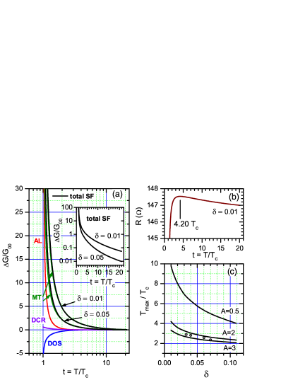
Figure 1: (Color online) (a) Temperature dependences of superconducting fluctuation contributions to conductivity [in the units of $G_{00}=e^{2}/(2\pi^{2}\hbar)$] GlatzVarVin . The curves for AL, DOS, and DCR processes are universal functions of reduced temperature $t=T/T_{c}$, the MT contribution is presented for $\delta=0.01$ and $0.05$. The black solid lines are the sum of all SF contributions Eq. (2). The inset shows the same total SF contribution on logarithmic scale. (b) Resistance vs. reduced temperature (see details in the text). (c) The set of the curves $T_{max}/T_{c}$ vs. $\delta$ for different coefficients $A$ from Eq. (3). The circles represent the measured $T_{max}$ and $T_{c}$ and $\delta$ obtained by fitting the experimental data (see the Table I and discussion in the text).

The following comments are in order. The calculations clearly demonstrate that at temperatures $T>2T_{c}$ the total fluctuation-induced conductivity with the great precision merely coincides with that given by the MT term. In other words, in this temperature range the sum of contributions $\Delta G^{AL}+\Delta G^{DOS}+\Delta G^{DCR}$=0. Moreover, the MT process dominates the fluctuation superconductivity down to temperatures $t-1\lesssim\delta$. At lower temperatures the AL contribution starts to become larger. The fact that MT is a leading process in a wide range of temperatures has already been emphasized in very early works by Maki Maki1968 and Thompson Thompson1970 and subsequent theoretical works AslVar1980 ; LarkinMT1980 . On the experimental side, numerous experimental studies that demonstrate that the magnetoresistance at $T>T_{c}$ is caused mainly by the suppression of the MT process Haesendonck1983 ; Gershenzon1983 ; Raffy1983 ; Santhanam1984 ; Bergmann1984 ; Gordon1984 ; Gordon1986 ; Brenig1986 ; WuLin1994 ; MTPtSi support this conclusion.

Next, it is the common view that the temperature range $(T-T_{c})/T_{c}\equiv t-1$ where superconducting fluctuations are relevant is defined by the so-called Ginzburg-Levanyuk parameter, $t-1\lesssim$Gi. Note that in the two-dimensional case Gi$=e^{2}R/(23\hbar)$ and as follows from (7) Gi$\approx\delta$. Therefore Gi defines only a narrow vicinity of $T_{c}$ where the AL term becomes dominant. What concerns the total SF contribution, it remains noticeable and positive even at temperatures well above $T_{c}$, as it is clearly demonstrated by the inset in Fig. 1a presenting the total SF contribution on logarithmic scale.

As the measurable quantity is the resistance, rather than the conductance, it is instructive to recast the calculated QCC into the temperature dependence of the resistance, $R(T)$. To this end, we use Eq. (7) which offers a reasonable estimate for $G_{0}=R^{-1}$ in Eq. (1). In Fig. 1b we show the temperature dependence of the resistance calculated as $R(t)=[\Sigma\Delta G^{(i)}(t)+G_{0}]^{-1}$ for $\delta=0.01$ yielding $G_{0}^{-1}=147\,\Omega$. We choose the temperature reference point at $T=20T_{c}$ assuming that all the contributions are practically zero at this temperature. Summing up all the QCC we took the coefficient $A=2$ in Eq. (3). One sees that although the SF contributions alone would have resulted in the monotonic behaviour of the resistance (with $dR/dT>0$), the contributions from WL and ID processes make $R(T)$ become non-monotonic and exhibit a maximum at the some temperature, $T_{max}$, of about of few $T_{c}$.

In Fig. 1c we plot the ratio $T_{max}/T_{c}$ as function of $\delta$ for three most common experimental situations where $A=3,\,2$ and $0.5$, corresponding to three sets of parameters $(a,p,A_{ID})$ in Eqs. (3) and (4): (1,2,1), (1,1,1), and (-1/2,1,1). The immediate important conclusion to be drawn from these plots is that the maximum in the $R(T)$ dependences for thin superconducting films is always present, even for the smallest values of the coefficient $A$. However, in relatively thick films this maximum can be disguised by the classical linear drop of the resistance with decreasing temperature. The next observation is that for all the realistic parameters of the film, the larger the resistance $R$ [i.e. the larger $\delta$ Eq. (7)], the closer $T_{max}$ moves to $T_{c}$, maintaining, nevertheless, that the ratio $T_{max}/T_{c}$ remains always larger than 2. It is noteworthy that the maximum lies in the domain where the SF are dominated by the Maki-Thompson contribution and that the maximum itself arises from the competition between the WL+ID and MT processes. In general, $T_{max}/T_{c}$ vs. $\delta$ curves relate the quantity $T_{max}$ which is the only characteristic point in the $R(T)$ dependence with the transition temperature $T_{c}$ and as such can serve as a set of calibrating curves for the express-determination of $T_{c}$, since $A$ can be estimated from the analysis of the resistance behaviour at high temperatures.

Now we turn to discussion of our experimental results. Figure 2a presents the temperature dependences of the resistance per square for four TiN films with different room temperature resistances. In all samples the resistances first grow upon decreasing the temperature from room temperature down, then reach the maximum value, $R_{max}$, at some temperature $T_{max}$ (see Table I), and, finally, decreases, with $T_{max}$ being approximately three times larger than the temperature where $R$ becomes immeasurably small. Before fitting the data with the theory of QCC, let us verify that the films in question are indeed quasi-two-dimensional with respect to the effects of the electron-electron interaction. We find $l_{T}\approx 2.5$ nm at $T=300$ K ($l_{T}>12$ nm at $T=10$ K). Therefore the condition of quasi-two-dimensionality, $d\lesssim l_{T}$, is satisfied at all temperatures down from 300 K. That is why the temperature behaviour of the conductance follows the logarithmic temperature dependence in accord with Eq. (3), see Fig. 2b. Solid lines in Fig. 2a,b account for all quantum contributions.

Table 1: Sample characteristics: $R_{300}$ is the resistance per square at $T=300$ K; $R_{max}$ is the resistance at the maximum point achieved at temperature $T=T_{max}$; $T_{c}$ is the critical temperature determined from the quantum contribution fits together with the pair-breaking parameter $\delta$ and the coefficient $A$ in Eq.(3); $T_{BKT}^{(I)}$ is determined from the power-law behavior of $I$-$V$ characteristics and $T_{BKT}^{(B)}$ is found from the flux flow resistance data. Note that the sample S01 is the same sample #1 in ref. SITTiNJETPL , where the higher $T_{c}=0.6$ K was found since only the AL contribution was taken into account.

Film	$R_{300}$	$R_{max}$	$T_{max}$	$T_{c}$	$\delta$	A	$T_{BKT}^{(I)}$	$T_{BKT}^{(B)}$
$\#$	k$\Omega$	k$\Omega$	K	K			K	K
S04	0.855	0.932	7.34	2.538	0.033	2.63	2.497	2.475
S03	2.52	3.74	3.55	1.260	0.040	2.63	1.147	1.115
S15	2.94	4.74	2.88	1.115	0.060	2.59	0.910	0.895
S01	3.75	10.25	1.23	0.521	0.070	2.71	—	0.380

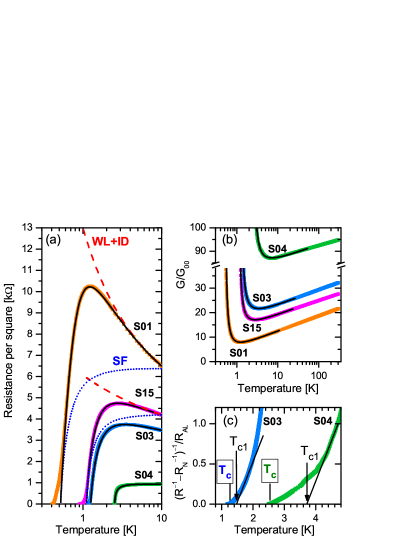
Figure 2: (Color online) (a) Resistance per square vs. temperature for four TiN film samples listed in Table I. Solid lines: fits accounting for all the corrections. Dashed lines (marked as WL+ID): separate contribution of the sum of weak localization and interaction in the diffusion channel to the resistance of the samples S01 and S15. Dotted lines (SF): contribution of superconducting fluctuations. (b) The same data as in (a), but extended to room temperatures and re-plotted as the dimensionless conductance $G/G_{00}$. The semi-logarithmic scale representation reveals logarithmic decrease of the conductance with temperature owing to WL and ID effects. (c) Reduced conductance $(R^{-1}-R_{N}^{-1})^{-1}/R_{AL}$ ($R_{AL}^{-1}=e^{2}/(16\hbar)$ and $R_{N}=R_{max}$) vs. $T$. The linear fit to the AL expression (solid lines) are often used for the determination of $T_{c}$ and generally gives incorrect (much too high) values of the critical temperature: $T_{c1}=1.470$ K, and $3.714$ K for samples S03 and S04, respectively (marked by arrows). The correct values of $T_{c}$ (presented in Table I) are in the rectangles and marked by the vertical bars.

The fitting remarkably captures all major features of the observed dependences: their non-monotonic behaviour, the position and the height of $R_{max}$, and the graduate decrease in the resistance matching perfectly the experimental points down to values $R\ll R_{max}$ (without any additional assumptions about mesoscopic inhomogeneities IoffeLarkin1981 ; Castellani2011 ). We were using three fitting parameters, $\delta$, $A$, and, $T_{c}$ (the values providing the best fit are given in the Table 1). It is noteworthy that while varying $\delta$ and $A$ significantly shifts the temperature position and the very value of $R_{max}$, it does not change noticeably the position of $T_{c}$. It reflects the fact that $\Delta G^{SF}$ does not depend on the pair-breaking parameter $\delta$ in the close vicinity of $T_{c}$ (see inset to Fig. 1a where the curves for different $\delta$ merge). A cross-check of the validity of the extracted values of $\delta$ and $A$ is achieved by taking the values of $T_{max}/T_{c}$ and $\delta$ found from fitting and superposing them on Fig. 1c. We see that the points fall between the lines corresponding to $A=2$ and $A=3$ in a nice accord with $A\simeq 2.6$ obtained from the full description of $R(T)$.

Having completed the full description of the experimental data within the framework of a general theory of superconducting fluctuations GlatzVarVin , it is instructive to review the approaches for inferring $T_{c}$ from the experimental data that were frequently used in the past. First, we find that $T_{c}$ lies at the foot of the $R(T)$ curve where $R(T)\simeq(0.08\div 0.13)R_{max}$. Therefore, the determination of $T_{c}$ as the temperature where $R(T)$ drops to 0.5$R_{N}$ (let alone to 0.9$R_{N}$) significantly overestimates $T_{c}$. Another frequently used procedure Fiory1983 is based on the assumption that the effect of quantum corrections can be reduced to the AL term only, i.e. that the resistance obeys the relation $R^{-1}=R_{N}^{-1}+R_{AL}^{-1}/(T/T_{c}-1)$, where $R_{AL}^{-1}=e^{2}/(16\hbar)=1.52\cdot 10^{-5}\,\Omega^{-1}$. This implies that there would have existed the range of temperatures near $T_{c}$ where the plot $[(R^{-1}-R_{N}^{-1})^{-1}/R_{AL}]$ vs. $T$ could have been approximated with a straight line with the slope $=1$. The intersection of this line with the $T$-axis would have defined $T_{c}$. Utilizing this approach we plotted in Fig. 2c the data for two of our samples, as an example, and indeed find such a linear dependence for each sample (shown by the solid lines), yielding temperatures of the intersections marked as $T_{c1}$. One sees, however, that this procedure gives much too high values for the superconducting critical temperatures.

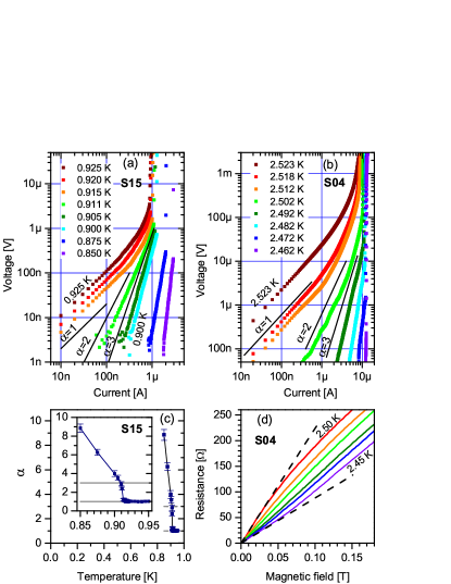
Figure 3: (Color online) Current-voltage characteristics on a double-logarithmic scale for samples S15 (a) and S04 (b) at different respective temperatures listed in the panels. Solid lines indicate the slopes corresponding to different values of power $\alpha$ on the $V\propto I^{\alpha}$. (c) $\alpha(T)$ for sample S15 in a full-temperature scale showing that the development of the power-law behaviour occurs over a very narrow temperature interval. The inset presents the same data on a magnified temperature scale, emphasizing the jump from $\alpha=1$ to $\alpha=3$ at the transition. (d) Resistance isotherms vs. magnetic field for sample S04 measured at temperatures 10 mK apart. The dashed lines are the tangents to lowest and highest isotherms stressing the evolution from superlinear to sublinear behaviour.

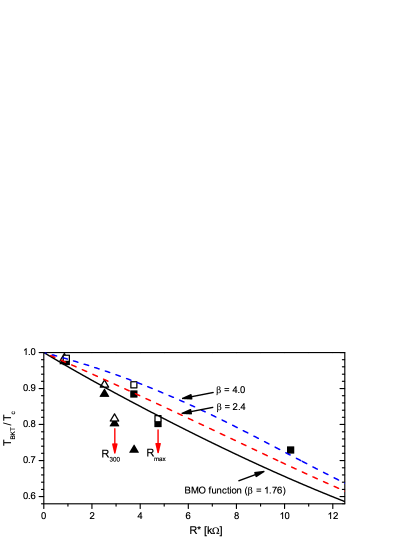
Figure 4: (Color online) Plot of $T_{BKT}/T_{c}$ as a function of $R^{*}$ for TiN films. The triangles correspond to $R^{*}=R_{300}$ and squares stand for $R^{*}=R_{max}$ giving better agreement with theory. Open symbols represent $T_{BKT}$ determined from the power-law behaviour of $I$-$V$ curves; closed symbols correspond to $T_{BKT}$ obtained from flux flow resistance data. The lines represent BMO functions (8) for different values of $\beta$ in (9).

We now turn to the determination of $T_{BKT}$ in our samples. There exists two distinct methods for finding $T_{BKT}$ from transport measurements. The first utilizes power-law fits to the $I$-$V$ characteristics of the film for which the switch from $V\propto I$ to $V\propto I^{3}$ occurs at the transition HalperinNelson1979 . Figures 3a,b show the typical sets of the $I$-$V$ curves for our samples at different temperatures near and below $T_{BKT}$ as log-log plots which indeed represent $V\propto I^{\alpha}$ behaviour, with $\alpha$ rapidly growing in a narrow temperature window, characteristic to the BKT transition (Fig. 3c). The values of $T_{BKT}^{(I)}$ determined as temperature where $\alpha=3$ are presented in the Table 1. Note that even at $T>T_{BKT}$ while $V\propto I$ at low currents, the $I$-$V$s become strongly nonlinear at elevated currents showing the characteristic rounding. In contrast to that at $T\leq T_{BKT}$ there is an abrupt voltage jump terminating the power-law behaviour at a certain well defined current. We attribute this jump to a heating instability in the low-temperature BKT phase, the nature of which along with the formation of the critical current in the BKT state will be discussed in a forthcoming publication GurVinBat .

The second technique for determining $T_{BKT}$ involves the use of flux flow resistance data Minnhagen1981 ; MinnhagenRevModPhys ; Fiory1983 ; HebardPaalanen1985 ; Simon1987 . Figure 3d shows a family of magnetoresistance isotherms typical for all our samples. With increase of temperature the $R(B)$ dependences progress from positive curvature through linear dependence to negative curvature. Below $T_{BKT}$ field-induced free vortices not only contribute to the resistance due to their own motion, but screen antivortices helping to dissociate vortex-antivortex pairs. This results in a superlinear response to the applied field. Above $T_{BKT}$ the vortex-antivortex pairs are unbound and all thermally induced vortices contribute to the resistance. Field-induced vortices annihilate with some fraction of antivortices, effectively reducing the number of vortices participating in the flux-flow, giving rise to a sublinear response to the applied field. The temperature of the linear response indicates thus $T_{BKT}$. The corresponding temperatures denoted as $T_{BKT}^{(B)}$ are listed in Table I. Note that while $T_{BKT}^{(B)}$ and $T_{BKT}^{(I)}$ are very close to each other, the former appears to be slightly lower than the corresponding values of $T_{BKT}^{(I)}$.

The summary of our results is presented in Fig. 4, showing the ratio of $T_{BKT}/T_{c}$ vs. $R_{300}$ and $R_{max}$. Irrespectively to the choice of the resistance, the more disordered the film (i.e. the closer the film is to the SIT), the farther apart $T_{BKT}$ from $T_{c}$ is. Using the dirty-limit formula which relates the two-dimensional magnetic screening length to the normal-state resistance $R_{N}$, Beasley, Mooij, and Orlando (BMO) Beasley1979 (see also HebardKotliar1989 ) proposed the universal expression for ratio $T_{BKT}/T_{c}$

$$\frac{T_{BKT}}{T_{c}}f^{-1}\left(\frac{T_{BKT}}{T_{c}}\right)=0.561\frac{\pi^{3}}{8}\left(\frac{\hbar}{e^{2}}\right)\frac{1}{R_{N}}\,,$$ (8)

$$f\left(\frac{T}{T_{c}}\right)=\frac{\Delta(T)}{\Delta(0)}\tanh\left[\frac{\beta\Delta(T)T_{c}}{2\Delta(0)T}\right]\,,$$ (9)

where $\Delta(T)$ is the temperature dependence of the superconducting gap and parameter $\beta=\Delta(0)/(k_{B}T_{c})$. The BCS theory predicts value $\beta=1.76$. The BMO function for this value of $\beta$ is shown by the solid line in Fig. 4 and correctly describes the qualitative tendency of decreasing the $T_{BKT}/T_{c}$ ratio with increasing disorder. The quantitative comparison however encounters some problems. The source of one of them is that since disordered films exhibit strong temperature dependence of the resistance the choice of what value is to be taken as the normal-state resistance, $R_{N}$ in Eq. (8), is not a priori obvious, see the extensive discussion of the ambiguity of the experimental definition of $R_{N}$ in HebardKotliar1989 . Indeed, we see that choosing $R_{300}$ as $R_{N}$, we obtain $T_{BKT}/T_{c}$ dropping much faster that what is predicted by the BMO formula. At the same time taking $R_{max}$ as normal state resistance yields a result more close to theory, see Fig. 4. Another source of discrepancy is that the BMO function contains the ratio $\Delta(0)/T_{c}$. As it is shown in ref. STM_TiN , where the TiN films close by the parameters to those investigated in the present work were studied, this ratio is unusually large as compared to its BCS value and grows on the approach to the SIT. The dashed lines in Fig. 4 show the BMO function for elevated values of $\beta$ and demonstrate that choosing values of $\beta$ corresponding to increasing disorder can improve the agreement between theory and experiment.

In conclusion, we demonstrated that the temperature dependence of the resistance of quasi-two-dimensional superconducting films, including its non-monotonic behaviour and the significant broadening of the transition is perfectly described by the theory of quantum contributions to conductivity. The analysis based on careful account of all contributions enabled a precise determination of the superconducting transition temperature. We found that the transition to the global phase-coherent superconducting state occurs via the Berezinskii-Kosterlitz-Thouless transition, and that the ratio $T_{BKT}/T_{c}$ follows the universal Beasley-Mooij-Orlando relation upon an appropriate choice of the normal state resistance and taking into account the non-BCS $\Delta(0)/T_{c}$ ratio in disordered films.

- (1) M. R. Beasley, J. E. Mooij, and T. P. Orlando, Phys. Rev. Lett. 42, 1165 (1979).
- (2) B. I. Halperin and D. R. Nelson, J. Low. Temp. Phys. 36, 599 (1979).
- (3) A. Larkin and A. Varlamov, Theory of Fluctuations in Superconductors (Clarendon Press, Oxford, 2005).
- (4) P. Minnhagen, Phys. Rev. B 23, 5745 (1981).
- (5) P. Minnhagen, Rev. Mod. Phys. 59, 1001 (1987).
- (6) K. Epstein, A. M. Goldman, and A. M. Kadin, Phys. Rev. Lett. 47, 534 (1981).
- (7) S. A. Wolf, D. U. Gubser, W. W. Fuller, J. C. Garland, and R. S. Newrock, Phys. Rev. Lett. 47, 1071 (1981).
- (8) A. M. Kadin, K. Epstein, and A. M. Goldman, Phys. Rev. B 27, 6691 (1983).
- (9) A. F. Hebard and A. T. Fiory, Phys. Rev. Lett. 50, 1603 (1983).
- (10) A. T. Fiory, A. F. Hebard, and W. I. Glaberson, Phys. Rev. B 28, 5075 (1983).
- (11) A. F. Hebard and M. A. Paalanen, Phys. Rev. Lett. 54, 2155 (1985).
- (12) R. W. Simon, B. J. Dalrymple, D. Van Vechten, W. W. Fuller, and S. A. Wolf, Phys. Rev. B 36, 1962 (1987).
- (13) A. Glatz, A. A. Varlamov, and V. M. Vinokur, EPL 94, 47005 (2011); Phys. Rev. B 84, 104510 (2011).
- (14) F. Pfuner, L. Degiorgi, T. I. Baturina, V. M. Vinokur, and M. R. Baklanov, New J. Phys. 11, 113017 (2009).
- (15) B. Sacépé, C. Chapelier, T. I. Baturina, V. M. Vinokur, M. R. Baklanov, and M. Sanquer, Phys. Rev. Lett. 101, 157006 (2008).
- (16) B. Sacépé, C. Chapelier, T. I. Baturina, V. M. Vinokur, M. R. Baklanov, and M. Sanquer, Nat. Commun. 1, 140 (2010).
- (17) T. I. Baturina et al., Phys. Rev. Lett. 99, 257003 (2007); Physica C 468, 316 (2008).
- (18) T. I. Baturina et al., JETP Lett. 88, 752 (2008).
- (19) V. M. Vinokur et al., Nature 452, 613 (2008).
- (20) J. S. Langer and T. Neal, Phys. Rev. Lett. 16, 984 (1966).
- (21) L. G. Aslamasov and A. I. Larkin, Phys. Tverd. Tela (Leningrad) 10, 1104 (1968) [Sov. Phys. Solid State 10, 875 (1968)]; Phys. Lett. 26A, 238 (1968).
- (22) M. Strongin, O. F. Kammerer, J. Crow, R. S. Thompson, and H. L. Fine, Phys. Rev. Lett. 20, 922 (1968).
- (23) K. Maki, Prog. Theor. Phys. 39, 897 (1968).
- (24) R. S. Thompson, Phys. Rev. B 1, 327 (1970).
- (25) L. P. Gor’kov, A. I. Larkin, and D. E. Khmel’nitskii, Pis’ma Zh. Eksp. Teor. Fiz 30, 248 (1979) [JETP Lett. 30, 228 (1979)].
- (26) L. G. Aslamasov and A. A. Varlamov, J. Low Temp. Phys. 38, 223 (1980).
- (27) A. I. Larkin, Pis’ma Zh. Eksp. Teor. Fiz. 31, 239 (1980) [JETP Lett. 31, 219 (1980)].
- (28) B. L. Altshuler, A. G. Aronov, and P. A. Lee, Phys. Rev. Lett. 44, 1288 (1980).
- (29) B. L. Altshuler and A. G. Aronov, in Electron-Electron Interactions in Disordered Systems, edited by A. L. Efros and M. Pollak (Elsevier Science B.V., New York, 1985).
- (30) A. M. Finkel’shtein, Zh. Eksp. Teor. Fiz. 84, 168 (1983) [Sov. Phys. JETP 57, 97 (1983)].
- (31) Y. Bruynseraede, M. Gijs, C. Van Haesendonck, and G. Deutscher, Phys. Rev. Lett. 50, 277 (1983).
- (32) M. E. Gershenzon, V. N. Gubankov, and Yu. E. Zhuravlev, Solid State Comm. 45, 87 (1983); Zh. Eksp. Teor. Fiz. 85, 287 (1983) [Sov. Phys. JETP 58, 167 (1983)].
- (33) H. Raffy, R. B. Laibowitz, P. Chaudhari, and S. Maekawa, Phys. Rev. B 28, 6607 (1983).
- (34) P. Santhanam and D. E. Prober, Phys. Rev. B 29, 3733 (1984).
- (35) G. Bergmann, Phys. Rev. B 29, 6114 (1984).
- (36) J. M. Gordon, C. J. Lobb, and M. Tinkham, Phys. Rev. B. 29, 5232 (1984).
- (37) J. M. Gordon and A. M. Goldman, Phys. Rev. B. 34, 1500 (1986).
- (38) W. Brenig, M. A. Paalanen, A. F. Hebard, and P. Wölfle, Phys. Rev. B 33, 1691 (1986).
- (39) C. Y. Wu and J. J. Lin, Phys. Rev. B 50, 385 (1994).
- (40) Z. D. Kvon, T. I. Baturina, R. A. Donaton, M. R. Baklanov, M. N. Kostrikin, K. Maex, E. B. Olshanetsky, and J. C. Portal, Physica B 284-288, 959 (2000).
- (41) T. I. Baturina, D. R. Islamov, J. Bentner, C. Strunk, M. R. Baklanov, and A. Satta, JETP Lett. 79, 337 (2004).
- (42) L. B. Ioffe and A. I. Larkin, Zh. Eksp. Teor. Fiz 81, 707 (1981) [Sov. Phys. JETP 54, 378 (1982)].
- (43) S. Caprara , M. Grilli, L. Benfatto, and C. Castellani, Phys. Rev. B 84, 014514 (2011).
- (44) A. Gurevich, V. M. Vinokur, T. I. Baturina, to be published.
- (45) A. F. Hebard and G. Kotliar, Phys. Rev. B 39, 4105 (1989).