Photometric Redshift Probability Distributions
for Galaxies in the SDSS DR8

Abstract

We present redshift probability distributions for galaxies in the SDSS DR8 imaging data. We used the nearest-neighbor weighting algorithm presented in Lima et al. (2008) and Cunha et al. (2009) to derive the ensemble redshift distribution $N(z$), and individual redshift probability distributions $P(z$) for galaxies with $r$$<$21.8. As part of this technique, we calculated weights for a set of training galaxies with known redshifts such that their density distribution in five dimensional color-magnitude space was proportional to that of the photometry-only sample, producing a nearly fair sample in that space. We then estimated the ensemble $N(z$) of the photometric sample by constructing a weighted histogram of the training set redshifts. We derived $P(z$)s for individual objects using the same technique, but limiting to training set objects from the local color-magnitude space around each photometric object. Using the $P(z$) for each galaxy, rather than an ensemble $N(z$), can reduce the statistical error in measurements that depend on the redshifts of individual galaxies. The spectroscopic training sample is substantially larger than that used for the DR7 release, and the newly added PRIMUS catalog is now the most important training set used in this analysis by a wide margin. We expect the primary source of error in the $N(z$) reconstruction is sample variance: the training sets are drawn from relatively small volumes of space. Using simulations we estimated the uncertainty in $N(z$) at a given redshift is $\sim$10-15%. The uncertainty on calculations incorporating $N(z$) or $P(z$) depends on how they are used; we discuss the case of weak lensing measurements. The $P(z$) catalog is publicly available from the SDSS website.

1 Introduction

Photometric redshifts are estimates of redshift derived using broad-band photometric observables such as magnitudes and colors (Baum, 1962; Puschell et al., 1982; Koo, 1985; Loh & Spillar, 1986; Connolly et al., 1995). Typically, the set of observables for a given galaxy are not sufficient to uniquely specify its redshift, but only a probability distribution, the $P(z$). These $P(z$)s are often relatively broad. For simplicity of use and interpretation, one commonly uses a single number, the photometric redshift, as the best estimate of a galaxy’s redshift. As several recent works have shown (Mandelbaum et al., 2008; Cunha et al., 2009; Wittman, 2009; Bordoloi et al., 2010; Abrahamse et al., 2011), the use of a single number to represent the photo-$z$ leads to biases. Working with the full $P(z$) for each galaxy yields better estimates of the overall redshift distribution, $N(z)$, and can decrease biases in cosmological analyses. We note that several public photo-$z$ codes exist that can produce a $P(z$) per galaxy, e.g. Le Phare (Arnouts et al., 1999; Ilbert et al., 2006), ZEBRA (Feldmann et al., 2006), BPZ (Coe et al., 2006), ArborZ (Gerdes et al., 2010), and our own method (Cunha et al., 2009), henceforth referred to as ProbWTS, which is an acronym for Probability Distributions from Weighted Training Sets. We use $P(z)_{w}$ when referring to the $P(z$)  derived from ProbWTS.

In this paper, we describe a $P(z$) catalog for objects detected in the Data Release 8 (SDSS DR8; Aihara et al., 2011) of the Sloan Digital Sky Survey III (SDSS III; Eisenstein et al., 2011). We use the method of Cunha et al. (2009), which was also applied to SDSS DR7 (Abazajian et al., 2009), with improvements in the training set and photometry. The DR7 catalog of Cunha et al. (2009) has been successfully used in cosmological analyses, allowing, for example, for the first measurement of the transverse BAO scale derived purely from angular information, i.e. without using the 3D power-spectrum (Carnero et al., 2011) and for the measurement of the growth of structure using photometric LRGs (Crocce et al., 2011).

This paper is organized as follows. In §2 we discuss the method and in §3,4,5 we describe the data and sample selection. In §6 we discuss the training set and in §7,8 we show our results, including information about their public release, and estimate errors. In §9, we discuss the proper usage of these results. As an example, we discuss the particular case of weak gravitational lensing calculations. Finally, in §10 we summarize our results.

2 Method

The algorithm is detailed in Lima et al. (2008) and Cunha et al. (2009). The method is to derive weights for a training set of spectroscopically confirmed galaxies such that the distribution of relevant quantities, such as magnitudes or colors, matches that of a set of galaxies without known redshifts, henceforth the photometric sample. Assuming these quantities correlate with redshift, and are the only relevant quantities for redshift determination, the resulting weighted redshift histogram is proportional to the redshift probability distribution $N(z$) of the photometric sample.

The weighting provides a key advantage over other training sample methods such as neural nets. Forcing the distributions of observables of the two samples to be proportional essentially creates a “fair sample” from the training set; this approach helps avoid the biases that can arise when the training and photometric samples have different properties. However, this technique does require that all areas of observable space populated by the photometric sample are also populated by the training set, at least at some low level.

2.1 Nearest-neighbor $P(z$) redshift estimators

2.1.1 Weights

In this section, we briefly review the weighting method of Lima et al. (2008), which is required for computing $P(z$). We define the weight, $w$, of a galaxy in the spectroscopic training set as the normalized ratio of the density of galaxies in the photometric sample to the density of training-set galaxies around the given galaxy. These densities are calculated in a local neighborhood in the space of photometric observables, e.g., multi-band magnitudes. In this case, the SDSS ugriz magnitudes are our observables; in practice we use four colors and the $r$–band magnitude. The hypervolume used to estimate the density is set to be the Euclidean distance of the galaxy to its $100^{th}$ nearest-neighbor in the training set.

The weights can be used to estimate the redshift distribution $N(z)_{\rm wei}$ of the photometric sample:

$$N(z)_{\rm wei}=\sum_{\beta=1}^{N_{\rm T}}w_{\beta}\delta(z-z_{\beta})~{}.$$ (1)

For a bin $z_{1}<z<z_{2}$, we sum the weights of all training set galaxies that fall within that bin. Lima et al. (2008) and Cunha et al. (2009) show that this indeed provides a nearly unbiased estimate of the redshift distribution of the photometric sample, $N(z)_{\rm P}$, provided the differences in the selection of the training and photometric samples are solely in the observable quantities used to calculate the weights. For example, if the photometric sample has a morphology dependent cut, the same cut should be applied to the training sample or morphology should be one of the observables used to measure weights.

2.1.2 $P(z$)

To estimate the redshift error distribution for each galaxy, $P(z$), we adopt the method of Cunha et al. (2009). The $P(z$) for a given object in the photometric sample is simply the redshift distribution of the $N$ nearest neighbors in the training set.

$$\hat{P}(z)=\sum_{\beta=1}^{N_{\rm nei}}w_{\beta}\delta(z-z_{\beta})~{}.$$ (2)

This expression is the same as Eqn. 1 but is limited to the nearest neighbors of a given object. We choose $N=100$ for this study, and estimate $P(z$) in 35 redshift bins between $z=0$ and 1.1. We can also construct a new estimator for $N(z)_{\rm P}$ by summing the $\hat{P}(z)$ distributions for all galaxies in the photometric sample,

$$N(z)_{\rm P}=\sum_{i=1}^{N_{\rm P,tot}}\hat{P}_{i}(z)~{}.$$ (3)

This estimator becomes identical to that of Eqn. (1) in the limit of very large training sets. For training sets smaller than tens of thousands of galaxies, one can improve the $P(z$)s by multiplying each $P(z$) by the ratio of $N(z)_{\rm wei}$ to $N(z)_{\rm P}$. That is,

$$P(z)\rightarrow P(z)\frac{N(z)_{\rm wei}}{N(z)_{\rm P}}$$ (4)

This correction essentially corresponds to using the weights estimate as a prior on the $P(z$)s.

3 Photometric Data

The photometric data were drawn from data release 8 (DR8) of the Sloan Digital Sky Survey III. Full details are given in the data release paper Aihara et al. (2011). As compared to the earlier DR7 release (Abazajian et al., 2009), DR8 includes an additional 2500 deg² of new imaging in the Southern Galactic Cap (SGC), acquired to facilitate spectroscopic target selection for the Baryon Oscillation Spectroscopic Survey (BOSS), which is part of SDSS III.

SDSS (York et al., 2000) images are gathered using the 2.5 meter at Apache Point (Gunn et al., 2006) with the camera (Gunn et al., 1998) running in time-delay-and-integrate mode. Observations are taken in each of the SDSS bandpasses (ugriz; Fukugita et al., 1996) nearly simultaneously as sky moves across bands in the order $riuzg$. The data were taken during photometric nights under relatively good seeing conditions (Hogg et al., 2001). A series of pipelines are run to calibrate the data (Padmanabhan et al., 2008; Smith et al., 2002; Tucker et al., 2006), derive astrometry (Pier et al., 2003), and calculate fluxes, shapes and other interesting quantities (Lupton et al., 2001). Note the calibrations used for these data are derived using the “ubercalibration” technique presented in Padmanabhan et al. (2008).

4 Photometric Quantities

In this section we describe the photometric quantities used in the creation of the input catalog. Most of these quantities are measured by the SDSS photometric pipeline PHOTO. An early version of the pipeline is described in Lupton et al. (2001); other details can be found in the SDSS Data Release papers, e.g. Adelman-McCarthy et al. (2006) and at the SDSS III website. We give a few additional details below. In comparison to DR7, the DR8 makes use of an updated version of the PHOTO software reduction pipeline, v5_6 rather than v5_4, including some updates to sky subtraction that can change galaxy photometry and, potentially, the $P(z$)s.

For colors we use the SDSS “model magnitudes”, which we refer to as modelmag. Each object is fit to an elliptical exponential disk and an elliptical De Vaucouleurs’ profile convolved with a double Gaussian approximation to the PSF model interpolated to the location of the object (Lupton et al., 2001; Sheldon et al., 2004). For the modelmag, the best fit model in the $r$ band is then used to extract the flux in the other four bandpasses, accounting appropriately for the PSF in each band. Thus the effective aperture is the same for all bands, which is appropriate for extraction of color information.

We use “composite model magnitudes” as an approximate total magnitude for each object, which we refer to as cmodelmag. For each bandpass separately, PHOTO does an additional joint fit to a non-negative linear combination of the best-fitting exponential and De Vaucouleurs’ models. This fit determines an additional parameter frac_deV ($f_{deV}$), which is the fraction of the total flux estimated to come from a De Vaucouleurs’ profile. The composite model flux in each band is then

$$\textrm{Flux}_{cmodel}\equiv(1-f_{dev})\times\textrm{Flux}_{exp}+f_{dev}\times\textrm{Flux}_{dev},$$ (5)

Because this procedure is carried out separately per band, the effective aperture for each band is different, so these magnitudes are not appropriate for estimating colors.

For quality assurance, we use bits from the OBJECT bitmask output by PHOTO. We also use the RESOLVE_STATUS to choose primary observations. We will describe how the flags are used in section §5.

5 Photometric Sample Selection

5.1 Star Galaxy Separation

The PHOTO pipeline uses the concentration $c$ to separate stars from galaxies. The concentration is the difference between magnitude determined from the best fitting PSF model psfmag and the modelmag  which is the better fitting of the exponential and De Vaucouleurs’ models convolved with the local PSF:

$$c\equiv\textrm{psfmag}-\textrm{modelmag}~{}.$$ (6)

For stellar objects, the scale of the modelmag approaches a delta function and the result becomes equivalent to the psfmag. Thus the concentration should be $\geq 0$ within the noise, with stars close to zero and galaxies greater than zero. The pipeline defines galaxies as objects with $c>0.145$ where $c$ is derived from the summed fluxes from all bandpasses.

At our magnitude limit $r=$21.8, the stellar contamination is relatively large. Using a small, space-based, high angular resolution data set matched to SDSS data as a truth table, the approximate stellar contamination can be determined. At $r$ = 21 the contamination is a few percent, but the contamination increases to approximately 10% at $r$ = 22.

For studies where completeness and purity must be known precisely, Scranton et al. (2005) recommend using probabilistic star galaxy separation at fainter mags ($r$ $>$ 21); i.e. attempt to determine the probability that an object is a galaxy and either use that as a weight or make appropriate cuts.

In practice the end user should choose a subset of the data that suits their needs. We provide a catalog here that should be a superset of objects that can be further trimmed.

5.2 Other Cuts

We remove objects for which the extinction-corrected (Schlegel et al., 1998) model flux is not well determined in at least one of the photometric bands. The adopted magnitude limits are [21, 22, 22, 20.5, 20.1] for $u,g,r,i,z$ respectively.

In addition to the magnitude limits described above, which ensures a reasonable detection in at least one band, we additionally demand a detection in both the $r$ and $i$ bands. Rather than applying a magnitude cut, we instead use the OBJECT processing flags BINNED{1,2,4}, which indicate the object was detected in the original image (binned by 1), the $\times$2 binned image, or the $\times$4 binned image, respectively(Stoughton et al., 2002).

We remove all objects that have the following OBJECT flags set: SATUR, BRIGHT, DEBLEND_TOO_MANY_PEAKS, PEAKCENTER, NOTCHECKED, NOPROFILE as well as objects that are (BLENDED && NODEBLEND); in other words, detected to be blended but not successfully deblended into components.

We only use objects marked as SURVEY_PRIMARY in their RESOLVE_STATUS flags field. Different scans on the sky image the same objects due to the small overlap regions between adjacent scans, overlaps at the end of the scan lines where the great circles converge, and re-observed scan lines. This results in duplicate observations for many objects. These duplicates are “resolved” and only a single observation is assigned SURVEY_PRIMARY. Note this primary also implies that, if the object is blended, it is either a child or not deblended further. This cut is made in the OBJECT flags as !BRIGHT && (!BLENDED || NODEBLEND || nchild == 0).

We require the extinction corrected (Schlegel et al., 1998) cmodelmag in the $r$ band to be in the range [15.0, 21.8]. We also restrict the extinction corrected modelmag to be within the range [15.0, 29.0] in order to ensure reasonable colors for the galaxies.

We make broad geometrical cuts on the catalog. We trim the objects to the BOSS footprint, shown in Fig. 1. We also remove any objects near stars in the tycho2 catalog (Høg et al., 2000) using a variable radius that depends on the magnitude of the star:

$$r=(0.0802\times B_{T}^{2}-1.860\times B_{T}+11.625)/60.0$$ (7)

where $B_{T}$ is the Tycho magnitude and $r$ is in degrees. Finally, we remove all objects from images taken where a $u$ amplifier was not working.

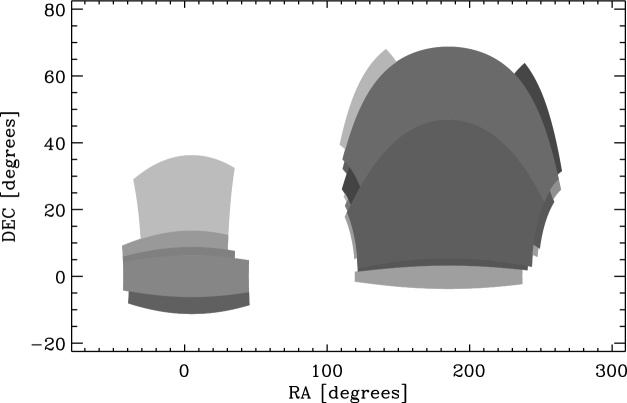
Figure 1: BOSS window function for the south galactic cap on the left and the north galactic cap on the right. The differently shaded regions represent contiguous rectangular regions in SDSS survey coordinates, used for construction of the window function. Note points with RA $>$ 300° have been wrapped below zero to avoid the 360° crossing point.

The final photometric catalog contains 58,533,603 objects. The distributions of extinction-corrected $r$-band cmodelmag and colors derived from extinction-corrected modelmag are shown in Fig. 2.

6 Training Samples

We use a spectroscopic training set drawn from a number of sources. These sources contain mostly galaxies and a small number of stars in order to help characterize stellar contaminants from the photometric sample at low redshift. In the following sections we give short details on each sample and describe our process for matching to the photometric sample.

6.1 Samples Used in this Study

• 435,878 redshifts from the SDSS spectroscopic samples, principally from the MAIN (Strauss et al., 2002) and Luminous Red Galaxy (LRG; Eisenstein et al., 2001) samples, with confidence level zconf$>0.9$, and r-band cmodelmag $<19.5$.

• 445 objects from the Canadian Network for Observational Cosmology (CNOC) Field Galaxy Survey (CNOC2; Yee et al., 2000) with Rval $>4$ for Sc$=2$ or Rval $>5$ for Sc$=5$

• 151 from the Canada-France Redshift Survey (CFRS; Lilly et al., 1995) with Class $\geq 3$.

• 1,868 from the Deep Extragalactic Evolutionary Probe 2 survey (DEEP2; Weiner et al., 2005) with zqual $\geq 3$. Of these, 1,499 are an approximately magnitude-limited sample from the Extended Groth Strip (EGS). The remainder is $BRI$ color-selected to target $z>0.7$ galaxies, hereafter denoted the non-EGS sample.

• 197 from the Team Keck Redshift Survey (TKRS; Wirth et al., 2004).

• 8,633 LRGs from the 2dF-SDSS LRG and QSO Survey (2SLAQ; Cannon et al., 2006) with qop $\geq$ 3.

• 2,080 from zCOSMOS redshift survey Lilly et al. (2007), with cc=3.4 || 3.5 || 4.4. || 4.5 || 9.5.

• 1,587 from the VIMOS VLT-Deep survey (VVDS; Garilli et al., 2008) with zqual $\geq 3$.

• 16,874 from four fields of the PRIMUS survey (PRIMUS; Coil et al., 2010; Cool et al., 2012). Only PRIMUS objects with $Q$ = 4 were used.

In table 1 we present some statistics about each training set.

6.2 Matching to SDSS Imaging Data

We spatially match the training sets listed in §6.1 to the photometric catalog described in §5. We choose the closest match within 2″. By performing this match we place the training set galaxies on the same photometric system as the photometric set. We also guarantee that the matches are drawn from the same magnitude range, and have the same quality cuts applied, as the photometric set.

As noted in §6.1, the training sets contain some stars. There are also stars in the photometric set, since the star galaxy separation is not perfect. Thus, through this matching between photometric set and training set it should be possible to place fraction of the stars in the photometric set at redshift zero; or at least some part of their derived $P(z$).

7 Results

We use the algorithm described in §2 to derive weights for each training set galaxy. We then use these weights to calculate a weighted redshift histogram which, under our assumptions, should be proportional to that of the photometric set. We also derive individual redshift probability distributions $P(z$) for each photometric galaxy.

7.1 Derived Weights in Observable Space

The $r$-band cmodelmag and colors based on modelmag for the photometric and training sets are shown in Fig. 2. Also shown are the derived weights for the training set and the resulting weighted histograms. These are the fundamentally new calculations presented in this work.

The weighted training set distributions should be approximately proportional to the photometric set distributions in order to derive good redshift distributions. There are deviations at $g-r$ $\sim 1.5$ and $r-i$ $\sim 0.6$, but qualitatively the distributions are close. We focus on the accuracy of the recovered redshift distributions rather than a detailed comparison of these distributions.

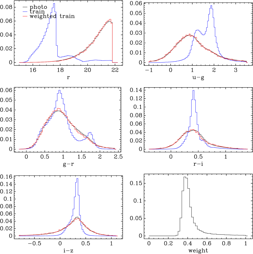
Figure 2: Distributions of photometric quantities for the photometric sample and training sample. The upper left panel shows the extinction-corrected $r$-band cmodelmag. Both samples are cut at $r$$<$21.8. Also shown is the weighted histogram for the training sample where the weights are derived to produced distributions approximately proportional to the photometric sample. The following four panels show extinction-corrected colors based on modelmag. The bottom right panel shows the distribution of of the derived weights for the training sample.

7.2 Derived $N(z$)

In figure 3 we present the recovered redshift distribution for the entire $r$ $<$ 21.8 sample. Also shown is the redshift distribution of the original training set. These distributions are in qualitative agreement with those shown in Cunha et al. (2009), although that sample had a fainter $r$-mag limit at 22.0. Note the sub-plot showing the region near $z=0$. As expected, there is a non-zero fraction of the overall distribution near redshift zero. The fraction of the probability at $z<0.002$ is about 0.4%. It is not known exactly how many stars are in the photometric sample, but this is probably a lower limit on the stellar contamination (see §5.1). We will estimate the errors on this distribution in §8. These $N(z$) data are presented in Table 2.

7.3 Derived $P(z$)

Also shown in Fig. 3 is the summed $P(z$) derived for individual galaxies. The uncorrected $N(z)_{\rm P}$ is, characteristically, slightly more peaked than than $N(z)_{\rm wei}$. In §7.3.1 we apply Eq. 4 to correct the $P(z$)s.

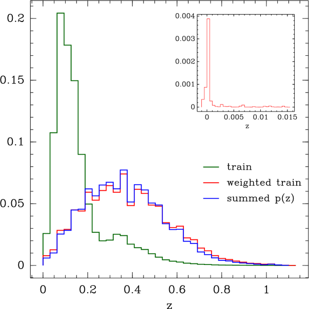
Figure 3: Reconstructed redshift distribution for SDSS galaxies with $r$ $<$ 21.8. The overall reconstructed distribution, shown in red, is derived by creating a weighted histogram of the training set redshifts as described in the text. Also shown in magenta is the sum of all $P(z$) derived for individual galaxies. The unweighted training set redshift distribution is shown in blue. The expected errors on these distributions from cosmic variance in the training set is shown in Fig. 8. The excess at $z\sim 0$ is due to stars in training set having significant weight; more detail at low redshift is shown in the inset. This excess is at least partly due to the presence of real stars in our photometric sample resulting from imperfect star-galaxy separation. The fraction of the distribution at $z<0.002$ is 0.4%, which is probably a lower bound on the stellar contamination.

In Fig. 4 we show six randomly chosen $P(z$)s. Each panel contains a $P(z$) drawn from a particular magnitude range in extinction-corrected $r$-band cmodelmag; these ranges are given in the figure caption. This figure captures the general trend that the $P(z$) are broader at fainter magnitudes, which is the expected behavior.

Figure 4: Six randomly chosen $P(z$)s. For each panel, an object was chosen from a particular magnitude range. Column-wise from top the left these ranges are $r<18$, $18<r<19$, $19<r<20$, $20<r<21$, $21<r<21.5$, $21.5<r<21.8$. The extinction-corrected $r$-band cmodelmag of each object is indicated in the upper right of each panel.

The uncertainty in individual $P(z$)s are typically dominated by shot-noise error. The scale of both statistical and systematic uncertainties in the individual $P(z$)s is strongly correlated with the width of the $P(z$) (Cunha et al., 2009). A broader $P(z$) reflects a larger degeneracy in observable space, and requires more training-set objects to characterize. Fig. 5 shows the distribution of objects in the photometric sample as a function of $r$-band magnitude and $1\sigma$ width of the $P(z$). The contours indicate factor of two changes in density.

We recommend using the $1\sigma$ or other width measures of the $P(z$) as the most efficient way to trim the sample for improved precision and accuracy. The $P(z$) width should also be a reasonable error estimator for use with other photo-$z$ methods. However, we discourage using the peak or some other single number statistic derived from the $P(z$) as a proxy for redshift. See §9 for more details.

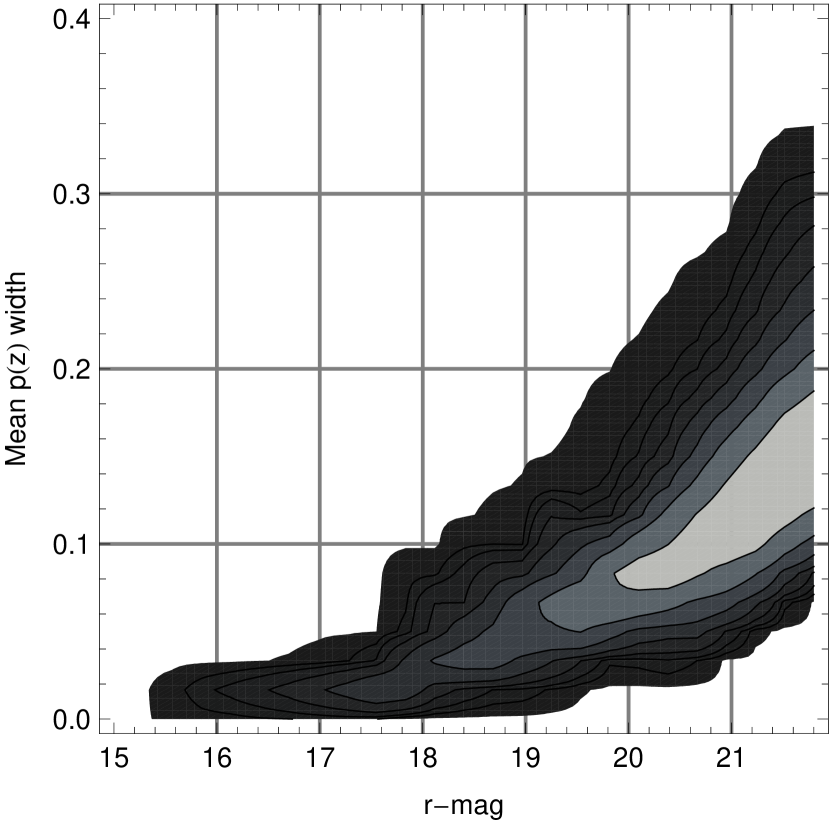
Figure 5: Density contours of the mean $P(z$) width as a function of r magnitude. The width of each $P(z$) is the defined as the standard deviation about the mean. The contours represent factors of 2 changes in density.

7.3.1 Correction to $P(z$)

As we will demonstrate in §9.1, the individual $P(z$)s are somewhat less accurate than the overall $N(z$). We can correct the individual $P(z$) to agree, in the mean, with the overall $N(z$) using Eqn. 4. This correction factor is shown in Figure 6. At $z\gtrsim 0.9$ neither the $N(z$) or the summed $P(z$) are well constrained, and the correction factor is noisy. For $z>0.9$ we use the average correction from that range.

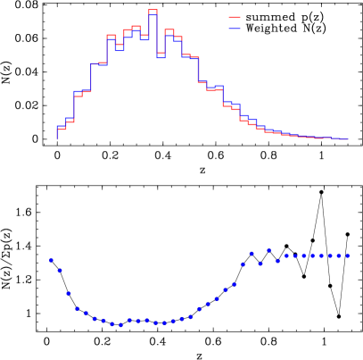
Figure 6: Correction factor from Eq. 4. This correction factor is the ratio of the $N(z$), which we find to be unbiased, to the summed $P(z$) from individual objects. The top panel shows both $N(z$) and $P(z$), and the bottom panel is the ratio. We apply this correction to each of the $P(z$)s in the release catalog. Note for $z>0.9$ we use the average correction from that range.

7.4 Differences from previous $P(z$) derived using this method

Unlike for the DR7 catalog, we did not use repeat observations of our training set galaxies. The use of repeats can provide more localized and smoother $P(z$) estimates, and are often useful. However, because only part of our sample had repeat observations, the use of repeats would effectively increase the sample variance of our results. The use of repeats may be beneficial for LRGs because the training set is not sample variance limited in this case. We may release a catalog trained on repeat observations at a future date.

7.5 Acquiring the Data

The $P(z$) for all galaxies are stored on the SDSS III website. The data are available in both FITS format and ASCII. The objects are split into different files according to their SDSS run id, with each row in the file representing the data for a single SDSS object. The data for each object are SDSS id, the input colors and magnitude for each object, equatorial latitude and longitude, and the estimated $P(z$).

8 Sources of Error

As detailed in Cunha et al. (2009), the derived weights, and inferred $N(z$), are susceptible to at least four kinds of training-set selection effects: spectroscopic failures, two types of large-scale structure bias (sample variance + shot noise in the training set), and selection in non-photometric observables. In addition, the fact that the weights use a non-infinitesimal volume in color-magnitude space to re-weight the photometric set can yield a small Eddington bias to the recovered distribution. And, as mentioned previously, incorrect star-galaxy separation can result in incompleteness and contamination of the sample. Because our training set consists of many different surveys with different characteristics, it is important to quantify the contribution of each to the overall result. Table 1 lists, for each of the surveys comprising the training set, the number of objects, the approximate area, and the fraction the survey contributes to the weighted estimate of the overall redshift distribution. This fraction is calculated by summing the weights assigned to objects in each survey and dividing by the sum of weights from the entire training set.

From Table 1, we see that PRIMUS carries the most weight by a large margin at 62%. Overall, the magnitude-limited surveys that reach our selection depth of 21.8 - PRIMUS, TKRS, CNOC2, DEEP2-EGS, CFRS, VVDS, and zCOSMOS - represent about 81$\%$ of the total weight. This is desirable, because it minimizes the risk of bias in our assessment of errors in what follows. The Table also shows that the SDSS MAIN sample ($r<17.8$) contributes only $1.7\%$ of the weights, which is consistent with the fraction expected from simulations for a flux-limited sample to $r<21.8$. The remainder of the SDSS spectra are LRGs to $r<19.4$, which make a contribution to the total weight at 7.4%.

In what follows, we identify potential sources of systematics and detail our tests to constrain them:

• Large-scale structure: We expect this item to be the main source of error. We use galaxy+$N$-body simulations to estimate the sample variance plus shot noise uncertainties of the spectroscopic redshift distributions of the training set. For simplicity, we only simulate the magnitude-limited surveys of the training set. In addition, because of the overlap between zCOSMOS and one of the PRIMUS fields, we neglect the zCOSMOS sample in the error estimation to simplify the calculation. This approach results in a $\sim$10% increase in the error bars relative to including zCOSMOS as an independent sample. The predicted error bars are overlayed on the simulated overall redshift distribution in Fig. 8, and the values of the errors are given in Table 2. The uncertainty in the training set redshift distributions is not identical to that of the uncertainty in the estimated redshift distributions $N(z$) derived using the weights, hence the error bars should be thought of as approximate. A more detailed estimation of the errors would require SDSS-specific photometry+$N$-body simulations. Relative to the error bars in the training set, the error bars in the weighted $N(z$) should be (very roughly) about 10-30% smaller, with increased anti-correlations between neighboring bins, but a more exact statement would require a significantly more detailed investigation. We explore these issues in more detail, and for a different data set, in Cunha et al. (2011).

• Selection in non-observables: Two of the surveys comprising our training set have selections in observables that are not included in the SDSS magnitude-limited sample. As mentioned previously, the DEEP2-nonEGS sample is selected using BRI photometry to target galaxies above $z>0.7$. As shown in Cunha et al. (2009), the use of DEEP2 in earlier versions of this catalog resulted in a bump in the overall estimated redshift distribution around $z\sim 0.8$. The present data release has a brighter magnitude cut and additional training data, which has eliminated this bias. DEEP2-nonEGS carries about 1.4% of the total weight. The 2SLAQ sample targets LRGs. Besides SDSS magnitudes, 2SLAQ also uses morphological information in the selection. Because shape correlates poorly with redshift, biases due to inclusion of the 2SLAQ sample are expected to be small. 2SLAQ is an important part of our sample because it provides a better training set for LRG’s at higher redshift than the SDSS sample.

• Spectroscopic redshift failures: The impact of spectroscopic failures is the most difficult to quantify. We chose a bright $r$-magnitude cut, and relatively stringent cuts on spectroscopic quality to minimize effects of failures, but it is possible that, for some applications, errors due to spectroscopic failures are not negligible. Based on the descriptions of the surveys comprising our training set, we expect the average completeness of our training sample to be well above $90\%$.

• Seeing: Nakajima et al. (2011) report that differences between the seeing distribution of the galaxies in the photometric and the training set can lead to biases in the photo-$z$ error calibration. In figure 7 we show the seeing distributions for all of our photometric sample compared to the four highest weight training samples, not including SDSS for which the seeing distribution is a near perfect match. The distributions are qualitatively similar, but with a trend to better seeing for the training set matches. More quantitatively, we checked the sensitivity of our results to seeing-induced biases by including seeing as a variable in the weights estimation. We find only negligible change in the recovered redshift distribution. Hence, although differences in seeing are in general a concern, we find little effect in our data.

For individual $P(z$)s, the main source of uncertainty is shot-noise, because only 100 galaxies were used to estimate each $P(z$). The choice to fix the number of neighbors keeps the shot-noise equal for all galaxies, but can yield biases or an artificial broadening of the $P(z$) if the training set is too sparse near the galaxy of interest. However, we do not find the volume spanned by the 100 nearest neighbors to be a good indicator of the $P(z$) quality, because other properties of the redshift-observable hyper-surface affect the local density of galaxies. A potentially more interesting indicator of bias in individual $P(z$) s is the spatial distribution of the training set nearest neighbors relative to the galaxy for which a $P(z$) is needed. We leave these explorations for a future work.

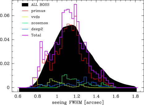
Figure 7: Distribution of seeing for the photometric sample (All BOSS) and the four most important training samples. These samples are important because they are magnitude limited and give relatively high weight in the analysis. Also shown is the sum of the training samples. The curves for each sample are normalized relative to the summed curve, and both the summed and photometric curves are normalized to unity.

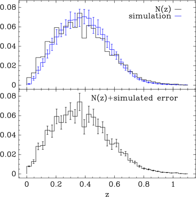
Figure 8: Top panel: Simulated redshift distribution with errors for an $r<$ 21.8 sample. The error bars are the $1\sigma$ simulated variability due to sample variance in the catalogs comprising the training set. Also shown is the estimated $N(z$) for our sample. Lower panel: estimated $N(z$) combined with the predicted sample variance errors from the simulation.

9 Proper Use

In this section we describe the proper use of these redshift distributions. We risk an overly pedantic discussion in order to ensure that past mistakes in these types of analyses are not repeated.

If one desires to use the $P(z$) to evaluate any non-linear function $F(z)$, one must integrate the function times the $P(z$) over the entire distribution; i.e. one must take the expectation value of the function. The reason is quite simple. In general a function evaluated at the expectation value of $z$ does not equal the expectation value of the function:

$$\langle F(z)\rangle\neq F(\langle z\rangle).$$ (8)

The expectation value of the function should be computed as follows:

$$\langle F\rangle=\int_{0}^{\infty}F(z)P(z)\mathrm{d}z.$$ (9)

It is not correct to simply take the effective redshift $\int z\,P(z)\,\mathrm{d}z$ and evaluate the function at that redshift.

This statement is true in most interesting science cases. An excellent example is in gravitational lensing, where one must estimate the “critical surface density” $\Sigma_{\mathrm{crit}}$, which determines the lensing strength of a given lens-source pair; the lensing deflection angle is proportional to $\Sigma^{-1}_{\mathrm{crit}}$. The function $\Sigma_{\mathrm{crit}}$ depends on the angular diameter distances to the lens, source and between lens and source in a non-linear manner. The proper estimator for a lens at redshift $z_{l}$ and source with $P(z_{s})$ is

$$\Sigma^{-1}_{\mathrm{crit}}(z_{l})=\int_{0}^{\infty}\Sigma_{\mathrm{crit}}^{-1}(z_{l},z_{s})P(z_{s})\mathrm{d}z_{s}.$$ (10)

9.1 $P(z$) and galaxy-galaxy lensing: proof-of-principle

The sensitivity of observational methods to the properties of the $P(z$) or $N(z$) depends on the details of how the observation is carried out. In this section, we use the galaxy-galaxy lensing calibration method from Mandelbaum et al. (2008) and Nakajima et al. (2011) as an example of determining this sensitivity. This methodology requires the use of a fair subsample of source galaxies with spectroscopic redshifts. For the purpose of this paper, we use the DEEP2 EGS region, in which there are 730 galaxies that (a) pass all cuts to be included in the SDSS source catalog from Mandelbaum et al. (2005), (b) have secure redshifts from DEEP2, and (c) pass the additional cut $r<21.5$. DEEP2 EGS is only one of the many training samples used in our analysis, so this exercise should be thought of as a proof-of-principle.

In brief, the quantities that we have measured are the expected calibration bias $b_{z}$ in the galaxy-galaxy lensing signal due to the method of estimating the source redshift (i.e., a multiplicative systematic error), and the degree to which the variance in the lensing signal deviates from the ideal variance we would achieve with optimal weighting by the true source redshift (large deviation results in increased statistical error). The increase in statistical error when we have degraded redshift information arises both from source misidentification, and also from deviations of the weights from the optimal $1/\Sigma_{\mathrm{crit}}^{2}$. Schematically, these two quantities can be determined via weighted sums over lens-source pairs $j$ (with weight $\tilde{w}_{j}$; in what follows, estimated quantities using approximate redshift information have a tilde, and ones that use the true redshift do not):

$$b_{z}+1=\frac{\sum_{j}\tilde{w}_{j}(\tilde{\Sigma}_{\mathrm{crit},j}/\Sigma_{\mathrm{crit},j})}{\sum_{j}\tilde{w}_{j}}$$ (11)

and

$$\textrm{Variance ratio}\equiv\frac{\textrm{Ideal variance}}{\textrm{Real variance}}=\frac{(\sum_{j}\sqrt{\tilde{w}_{j}w_{j}})^{2}}{(\sum_{j}w_{j})(\sum_{j}\tilde{w}_{j})}.$$ (12)

For more detail, see the aforementioned papers.

In Figure 9 we show the results of these calculations for several test cases. First, the red short-dashed curve provides, as a baseline, the calibration bias (top) and variance ratio (bottom) when using the ZEBRA photo-$z$ studied in Nakajima et al. (2011). As shown, there is a significant bias in the lensing signal that must be calibrated. Next, the green long-dashed line shows what happens if we use the $N(z)_{\mathrm{wei}}$ as an estimate of the redshift distribution, rather than using any individual galaxy photo-$z$ or $P(z$) information. Crucially, the lensing signal is unbiased in this case. However, as shown in the bottom panel, we do find an increased statistical error due to lack of redshift information on a per-galaxy basis.

Third, the solid black line demonstrates what happens when we use the individual $P(z$)s to estimate $\Sigma_{\mathrm{crit}}$ using Eq. 10. These $P(z$)s are derived from a very specific, idealized case, using only EGS both as the training sample and the photometric sample. In this case, the individual $P(z$)s are on average $40\%$ broader than the DR8 $P(z$)s because of the use of 100 neighbors to construct each $P(z$) when the training sample itself is only $7$ times as large. To compensate for the bias introduced by the small size of the training sample, we have imposed a multiplicative correction factor to the $P(z$)s such that $\sum P(z)=N(z)_{\mathrm{wei}}$ using Eq. 4. Nonetheless, there is a calibration bias due to the very significant width of the $P(z$)s (which can be removed using a calibration sample); but the variance ratio is still far closer to optimal than when we did not use weighting information, and slightly closer than when we used ZEBRA photo-$z$.

The magenta dot-dashed line shows the results when 7 neighbors are used to estimate the $P(z$), not including the galaxy itself. The blue dot-long dashed line shows the same case but with the Eq. 4 correction. This use of 7 neighbors reduces the abnormally broad $P(z$)s caused by using such a small training sample and 100 neighbors. The mean $P(z$) width for the 7 neighbors case is 0.0989, to be compared to the mean width of the DR8 $P(z$)s of 0.0983. The calibration bias for 7 neighbors is also quite close to the ideal case with $N(z)_{\mathrm{wei}}$, and the weighting is the closest to optimal of all the cases considered in this paper.

To summarize, we have demonstrated for this simplified training set that, for the purpose of lensing, we achieve a perfect signal calibration when using $N(z)_{\mathrm{wei}}$; i.e., no individual galaxy redshift information. However, the weighting is suboptimal. When we use individual $P(z$)s, the lensing signal can be biased due to their finite width even if $\sum P(z)=N(z)_{\mathrm{wei}}$, but this bias can be calibrated. The advantage of using individual $P(z$) information is that statistical errors on the lensing signal are reduced due to more optimal weighting. This is because a signal-to-noise ratio weighting is proportional to $\langle\Sigma_{\mathrm{crit}}^{-2}\rangle$, so sources expected to be behind the lens are given higher weight than those expected to be close to or in front of the lens.

Again, we emphasize that this analysis used only DEEP2 EGS, and should be used as a proof-of-principle to gain intuition. Users of these data should perform similar analyses to these but matched to their exact analysis and selection criteria.

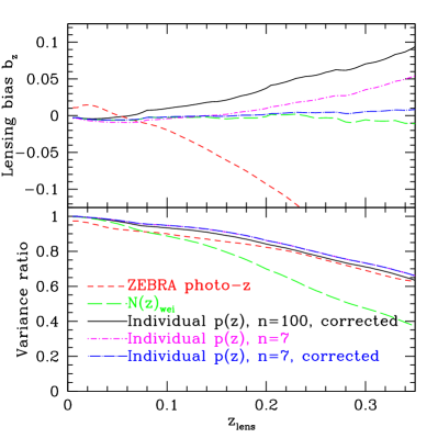
Figure 9: Proof-of-concept analysis of errors in a fictitious lensing analysis. For this example we used only DEEP2-EGS galaxies but perfect weights estimate; the sample variance and width of individual $P(z$)s are much larger than for the DR8 analysis. Top: Lensing signal calibration bias (Eq. 11) as a function of lens redshift, for four cases labeled on the plot and discussed in the text. Bottom: Ratio of the ideal to the real signal variance when using different methods of redshift determination; the goal is to stay as close to unity as possible.

10 Summary

In this paper we presented a catalog of photometric redshift probability distributions for the SDSS DR8. With some modifications, our method is the same as that used to generate the $P(z$) catalog for SDSS DR7, presented in Cunha et al. (2009). For this catalog, we used the ubercal photometry (Padmanabhan et al., 2008). We also included the PRIMUS galaxy sample, which more than doubles the number of galaxies in our training set that are drawn from a flux-limited sample other than SDSS. The addition of PRIMUS provided a significant increase in the total area of the non-SDSS training set, which reduces the sample variance. We examined several potential sources of error, including shot noise, sample variance, seeing, star-galaxy separation, and spectroscopic failures. We expect that sample variance is the main source of uncertainty in our overall redshift distribution. For individual $P(z$)s, shot-noise is the limiting uncertainty, since each $P(z$) is based on 100 training set galaxies. These $P(z$)s, and the ensemble $N(z$) derived in this work (Table 2), should be useful for a variety of science applications, such as galaxy angular two-point correlation functions, galaxy cluster detection and weak gravitational lensing.

Table 1: Statistics for Each Training Set

Survey	Number	Area	Weight Fraction
	of Objects	(sq. deg.)
PRIMUS∗	16,874	5.2	0.63
zCOSMOS∗	2,080	1.7	0.075
SDSS DR5	435,875	5740	0.074
2SLAQ	8,633	180	0.060
VVDS∗	1,587	4.0	0.060
DEEP2-EGS∗	1,499	0.4	0.058
SDSS DR5 ($r<17.8$)	376,625	5740	0.017
CNOC2∗	445	0.4	0.016
DEEP2-nonEGS∗	369	2.8	0.014
CFRS∗	151	$<$0.1	0.0076
TKRS∗	197	0.07	0.0055

Note. — Number of galaxies, area in square degrees, and fractional contribution to the weights estimate of $N(z)$. The “*” indicates samples that are approximately flux-limited to our selection depth.

Table 2: Estimated $N(z$) and Sample Variance Errors

$z_{min}$	$z_{max}$	$N(z$)	Sample Variance
			Error
0.000	0.031	0.788	0.045
0.031	0.063	1.267	0.195
0.063	0.094	2.841	0.346
0.094	0.126	2.921	0.396
0.126	0.157	4.496	0.429
0.157	0.189	4.407	0.636
0.189	0.220	5.920	0.756
0.220	0.251	5.293	0.689
0.251	0.283	6.065	0.791
0.283	0.314	6.464	0.863
0.314	0.346	5.926	0.696
0.346	0.377	7.407	0.889
0.377	0.409	4.845	0.745
0.409	0.440	6.147	0.827
0.440	0.471	5.845	0.827
0.471	0.503	4.890	0.763
0.503	0.534	4.797	0.572
0.534	0.566	3.466	0.586
0.566	0.597	3.066	0.548
0.597	0.629	3.178	0.388
0.629	0.660	2.229	0.293
0.660	0.691	2.085	0.228
0.691	0.723	1.406	0.183
0.723	0.754	1.185	0.141
0.754	0.786	0.795	0.093
0.786	0.817	0.564	0.070
0.817	0.849	0.477	0.054
0.849	0.880	0.354	0.039
0.880	0.911	0.268	0.029
0.911	0.943	0.181	0.024
0.943	0.974	0.152	0.020
0.974	1.006	0.103	0.016
1.006	1.037	0.115	0.013
1.037	1.069	0.042	0.011
1.069	1.100	0.015	0.010

Note. — Reconstructed redshift distribution $N(z$) for SDSS galaxies with $r$ $<$ 21.8. The first two columns specify the redshift range of the bin and the third is the reconstructed $N(z$), with arbitrary normalization. The fourth is the sample variance errors on $N(z$) derived from simulations, which we expect to be the dominant uncertainty. These sample variance errors should be thought of as a rough estimate. A more perfect match would require a simulation more specifically tuned to the SDSS data.

References

- Abazajian et al. (2009) Abazajian, K. N. et al. 2009, ApJS, 182, 543
- Abrahamse et al. (2011) Abrahamse, A., Knox, L., Schmidt, S., Thorman, P., Tyson, J. A., & Zhan, H. 2011, ApJ, 734, 36
- Adelman-McCarthy et al. (2006) Adelman-McCarthy, J. K. et al. 2006, ApJS, 162, 38
- Aihara et al. (2011) Aihara, H. et al. 2011, ApJS, 193, 29
- Arnouts et al. (1999) Arnouts, S., Cristiani, S., Moscardini, L., Matarrese, S., Lucchin, F., Fontana, A., & Giallongo, E. 1999, MNRAS, 310, 540
- Baum (1962) Baum, W. A. 1962, in IAU Symposium, Vol. 15, Problems of Extra-Galactic Research, ed. G. C. McVittie, 390–+
- Bordoloi et al. (2010) Bordoloi, R., Lilly, S. J., & Amara, A. 2010, MNRAS, 406, 881
- Busha et al. (2011) Busha, M., Wechsler, R., et al. 2011, in preparation
- Cannon et al. (2006) Cannon, R. et al. 2006, MNRAS, 372, 425
- Carnero et al. (2011) Carnero, A., Sanchez, E., Crocce, M., Cabre, A., & Gaztanaga, E. 2011, ArXiv e-prints
- Coe et al. (2006) Coe, D., Benítez, N., Sánchez, S. F., Jee, M., Bouwens, R., & Ford, H. 2006, AJ, 132, 926
- Coil et al. (2010) Coil, A. L., Blanton, M. R., Burles, S. M., Cool, R. J., Eisenstein, D. J., Moustakas, J., Wong, K. C., Zhu, G., Aird, J., Bernstein, R. A., Bolton, A. S., & Hogg, D. W. 2010, ArXiv e-prints
- Connolly et al. (1995) Connolly, A. J., Csabai, I., Szalay, A. S., Koo, D. C., Kron, R. G., & Munn, J. A. 1995, AJ, 110, 2655
- Cool et al. (2012) Cool, R. et al. 2012, in preparation
- Crocce et al. (2011) Crocce, M., Gaztanaga, E., Cabre, A., Carnero, A., & Sanchez, E. 2011, ArXiv e-prints
- Cunha et al. (2011) Cunha, C. E., Huterer, D., Busha, M., & Wechsler, R. 2011, in preparation
- Cunha et al. (2009) Cunha, C. E., Lima, M., Oyaizu, H., Frieman, J., & Lin, H. 2009, MNRAS, 396, 2379
- Eisenstein et al. (2001) Eisenstein, D. J. et al. 2001, AJ, 122, 2267
- Eisenstein et al. (2011) —. 2011, ArXiv e-prints
- Feldmann et al. (2006) Feldmann, R., Carollo, C. M., Porciani, C., Lilly, S. J., Capak, P., Taniguchi, Y., Le Fèvre, O., Renzini, A., Scoville, N., Ajiki, M., Aussel, H., Contini, T., McCracken, H., Mobasher, B., Murayama, T., Sanders, D., Sasaki, S., Scarlata, C., Scodeggio, M., Shioya, Y., Silverman, J., Takahashi, M., Thompson, D., & Zamorani, G. 2006, MNRAS, 372, 565
- Fukugita et al. (1996) Fukugita, M. et al. 1996, AJ, 111, 1748
- Garilli et al. (2008) Garilli, B. et al. 2008, A&A, 486, 683
- Gerdes et al. (2010) Gerdes, D. W., Sypniewski, A. J., McKay, T. A., Hao, J., Weis, M. R., Wechsler, R. H., & Busha, M. T. 2010, ApJ, 715, 823
- Gunn et al. (1998) Gunn, J. E. et al. 1998, AJ, 116, 3040
- Gunn et al. (2006) —. 2006, AJ, 131, 2332
- Høg et al. (2000) Høg, E., Fabricius, C., Makarov, V. V., Urban, S., Corbin, T., Wycoff, G., Bastian, U., Schwekendiek, P., & Wicenec, A. 2000, A&A, 355, L27
- Hogg et al. (2001) Hogg, D. W., Finkbeiner, D. P., Schlegel, D. J., & Gunn, J. E. 2001, AJ, 122, 2129
- Ilbert et al. (2006) Ilbert, O. et al. 2006, A&A, 457, 841
- Koo (1985) Koo, D. C. 1985, AJ, 90, 418
- Lilly et al. (1995) Lilly, S. J., Le Fevre, O., Crampton, D., Hammer, F., & Tresse, L. 1995, ApJ, 455, 50+
- Lilly et al. (2007) Lilly, S. J. et al. 2007, ApJS, 172, 70
- Lima et al. (2008) Lima, M., Cunha, C. E., Oyaizu, H., Frieman, J., Lin, H., & Sheldon, E. S. 2008, MNRAS, 390, 118
- Loh & Spillar (1986) Loh, E. D. & Spillar, E. J. 1986, ApJ, 303, 154
- Lupton et al. (2001) Lupton, R. H. et al. 2001, in ASP Conf. Ser. 238: Astronomical Data Analysis Software and Systems X, 269–+ (astro–ph/0101420)
- Mandelbaum et al. (2008) Mandelbaum, R., Seljak, U., Hirata, C. M., Bardelli, S., Bolzonella, M., Bongiorno, A., Carollo, M., Contini, T., Cunha, C. E., Garilli, B., Iovino, A., Kampczyk, P., Kneib, J.-P., Knobel, C., Koo, D. C., Lamareille, F., Le Fèvre, O., Le Borgne, J.-F., Lilly, S. J., Maier, C., Mainieri, V., Mignoli, M., Newman, J. A., Oesch, P. A., Perez-Montero, E., Ricciardelli, E., Scodeggio, M., Silverman, J., & Tasca, L. 2008, MNRAS, 386, 781
- Mandelbaum et al. (2005) Mandelbaum, R. et al. 2005, MNRAS, 361, 1287
- Nakajima et al. (2011) Nakajima, R., Mandelbaum, R., Seljak, U., Cohn, J. D., Reyes, R., & Cool, R. 2011, ArXiv e-prints
- Padmanabhan et al. (2008) Padmanabhan, N. et al. 2008, ApJ, 674, 1217
- Pier et al. (2003) Pier, J. R. et al. 2003, AJ, 125, 1559
- Puschell et al. (1982) Puschell, J. J., Owen, F. N., & Laing, R. A. 1982, ApJ, 257, L57
- Schlegel et al. (1998) Schlegel, D. J., Finkbeiner, D. P., & Davis, M. 1998, ApJ, 500, 525+
- Scranton et al. (2005) Scranton, R. et al. 2005, ApJ, 633, 589
- Sheldon et al. (2004) Sheldon, E. S. et al. 2004, AJ, 127, 2544
- Smith et al. (2002) Smith, J. A. et al. 2002, AJ, 123, 2121
- Stoughton et al. (2002) Stoughton, C. et al. 2002, AJ, 123, 485
- Strauss et al. (2002) Strauss, M. A. et al. 2002, AJ, 124, 1810
- Tucker et al. (2006) Tucker, D. L. et al. 2006, Astronomische Nachrichten, 327, 821
- Weiner et al. (2005) Weiner, B. J. et al. 2005, ApJ, 620, 595
- Wirth et al. (2004) Wirth, G. D. et al. 2004, AJ, 127, 3121
- Wittman (2009) Wittman, D. 2009, ApJ, 700, L174
- Yee et al. (2000) Yee, H. K. C. et al. 2000, ApJS, 129, 475
- York et al. (2000) York, D. G. et al. 2000, AJ, 120, 1579