Statistical hadronization with exclusive channels in $\textrm{e}^{+}\textrm{e}^{-}$ annihilation

Abstract

We perform a systematic analysis of exclusive hadronic channels in $\textrm{e}^{+}\textrm{e}^{-}$ collisions at centre-of-mass energies between 2.1 and 2.6 GeV within the statistical hadronization model. Because of the low multiplicities involved, calculations have been carried out in the full microcanonical ensemble, including conservation of energy-momentum, angular momentum, parity, isospin, and all relevant charges. We show that the data is in an overall good agreement with the model for an energy density of about 0.5 GeV/fm³ and an extra strangeness suppression parameter $\gamma_{S}\sim 0.7$, essentially the same values found with fits to inclusive multiplicities at higher energy.

I Introduction

The statistical approach to multi-hadron production $\textrm{e}^{+}\textrm{e}^{-}$ annihilations has a long story. Early works date back to the ’70s eestat ; eestat2 , with different versions of the model and different observables examined in the relevant analyses, such as inclusive yields, multiplicity distributions etc. All of these calculations involved simplifying assumptions and drastic approximations, mostly because of the lack of computing power, so that in practice it was very difficult to confirm or rule out the statistical model, also in view of it being conceived as a full alternative to a dynamical model. Nowadays, with QCD being the accepted theory of strong interactions, the Statistical Hadronization Model (SHM) has resurged as a model of hadronization, it has a framework based on quantum statistical mechanics review , and it has been extensively and succesfully applied to the analysis of inclusive multiplicities in elementary vari and relativistic heavy ion collisions varih . Also, the SHM was shown to succesfully reproduce transverse momentum spectra in hadronic collisions becagp with specific predictions concerning the approximately exponential shape of the low-$p_{T}$ spectrum and the so-called $m_{T}$ scaling phenomenon. This model has by now become a standard tool in heavy ion physics while the reasons of its success in elementary collisions are still subject of debate diba .

It is a common belief that statistical equilibrium cannot be attained in elementary collisions via post-hadronization collisions because of the low multiplicities and the rapid expansion. Therefore, one is led to conclude that statistical equilibrium is an intrinsic feature of the hadronization process itself, as envisaged by Hagedorn many years ago (”hadrons are born at equilibrium” hage ). In the latter case, two possibilities arise:

• - the apparent statistical equilibrium is just mimicked by a special property of the dynamics governing the hadronization tending to evenly populates all final states, but which has essentially nothing to do with a proper statistical system, which can be realized only within a finite volume.

• - the apparent statistical equilibrium is established within a finite volume and therefore is a ”genuine” one; if the volume was large enough, a proper temperature could be introduced.

The former picture can be defined as phase space dominance to discriminate it from proper statistical equilibrium. While phase space dominance is, though, a highly non-trivial hypothesis, its predictions do quantitatively differ from the proper SHM. As pointed out in refs. meaning ; review , the dynamical matrix element of the decay of a massive cluster into $N$ particles contain, in the SHM case, peculiar quantum statistics terms (Bose-Einstein and Fermi-Dirac correlations) owing to the finite cluster volume, which are generally absent in the phase space dominance picture. The very fact that Bose-Einstein and Fermi-Dirac correlations have been observed in elementary collisions demonstrates the finite extension of the hadron emitting source and therefore favours a model like the SHM where finite volume is a built-in feature.

Anyhow, it would be desirable to quantitatively test the the genuine statistical hadronization model on observables which are more sensitive to the form of the matrix element than average multiplicities. For this purpose, in this work we compare the production rates of exclusive channels in $\textrm{e}^{+}\textrm{e}^{-}$ collisions at low energy with the predictions of the SHM.

Exclusive channels in $\textrm{e}^{+}\textrm{e}^{-}$ collisions have been measured at low centre-of-mass energy ($\lesssim 4$ GeV). At such a low energy, QCD is in the full non-perturbative regime and one can assume that, unlike at higher energy where clusters are two or more (jettiness), only one hadronizing massive cluster at rest in centre-of-mass frame of the collision is forme. The price to be paid is that, in calculating the model predictions, none of the relevant conservation laws, including energy-momentum, intrinsic angular-momentum and parity, as well as internal symmetries, can be neglected (see e.g. ref. heinzppb where $\textrm{p}\overline{\textrm{p}}$  annihilation at rest was studied in the SHM). In the SHM framework, this means that one has to calculate averages in the most general microcanonical ensemble of the hadron-resonance gas.

To carry out this calculation, in this work we take advantage of the formalism developed in two previous papers of ours bf3 ; bf4 where the microcanonical partition function of an ideal multi-species relativistic gas was calculated enforcing the conservation of the maximal set of observables pertaining to space-time symmetries (energy-momentum, spin, helicity, parity). We extend the formulae obtained therein to the hadron-resonance gas including internal quantities conserved by strong interaction (isospin, C-parity and abelian charges). We then take into account resonance decays and compare the results of our calculations with the data collected in $\textrm{e}^{+}\textrm{e}^{-}$ collisions at low energy.

The paper is organized as follows: in Sect. II we will expound a formulation of the SHM in the full microcanonical ensemble which is suitable for the problem of exclusive channels and in Sect. III we will obtain an expression for the their rates; Sect. IV will be focussed on a method to compute them numerically. Finally, Sect. V will describe the analysis of data in $\textrm{e}^{+}\textrm{e}^{-}$ collisions at low energy will and Sect. VI will be devoted to a discussion of the results and to conclusions.

II The Statistical Hadronization Model in the microcanonical ensemble

In the modern formulation of the SHM review , the strong interaction process in a collision between particles leads to the formation of a set of extended massive objects called clusters or fireballs). Each cluster decays into hadrons in a purely statistical fashion, that is any multi-hadronic state within the cluster compatible with its quantum numbers is equally likely. The number of clusters produced, as well as their kinematical and internal quantum properties, are determined by the prior dynamical process and are not predictable within the SHM itself. Particularly, in high energy collisions ($\sqrt{s}\gtrsim 10$ GeV), the production of clusters following the perturbative parton shower stage leads to a multiple cluster production. Conversely, for energies sufficiently below the perturbative regime ($\sqrt{s}\lesssim 4$ GeV), one may expect that, to a very good approximation, a single cluster is formed (see fig. 1). Under this circumstance the whole centre-of-mass energy is spent to produce particles and no jet is observed. The cluster mass will then coincide with $\sqrt{s}$ and its relevant quantum numbers will be the same as those pertaining to the initial state of the collision.

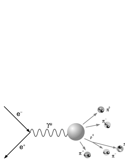
Figure 1: Dominant contribution to hadroproduction in a low energy $\textrm{e}^{+}\textrm{e}^{-}$ collision with formation of a single hadronizing cluster.

Once the quantum numbers of a cluster are known, the assumption of equal probability allows to perform calculations within the framework of statistical mechanics, in the relativistic microcanonical ensemble. The use of the microcanonical ensemble is necessary as at such a low energy the effect of exact conservation laws is very importantbf2 . It should be emphasized that the basic assumption of the model states that multi-particle localized states compatible with cluster’s conserved quantities are equally likely, but these states do not coincide with observable free particle asymptotic states. Such a distinction is, for practical purposes, not an issue when the volume is sufficiently large, but it is relevant in principle and may result in quantitative differences when the volume is small, i.e. comparable with the third power of the typical lenght scale of the hadron world, the pion Compton wavelength ${\mathcal{O}}(1)$ fm³. This is discussed in detail in refs. meaning ; review .

If the cluster can be described as a mixture of states, the basic postulate implies that the corresponding density operator is a sum over all localized states projected onto the initial cluster’s quantum numbers through a projection operator ${\sf P}_{i}$:

$$\widehat{\rho}\propto\sum_{h_{V}}{\sf P}_{i}|h_{V}\rangle\langle h_{V}|{\sf P}_{i}\equiv{\sf P}_{i}{\sf P}_{V}{\sf P}_{i}$$ (1)

where $|h_{V}\rangle$ are multi-hadronic localized states and ${\sf P}_{i}$ is the projector onto the cluster’s initial conserved quantities: energy-momentum, intrinsic angular momentum and its third component, parity and the generators of inner symmetries of strong interactions . If, on the other hand, the cluster is prepared in a pure quantum state $|\psi\rangle$(what is the case for a single produced cluster in $\textrm{e}^{+}\textrm{e}^{-}$ collisions) then, according to the basic assumption, this is ought to be an even superposition of all multi-particle localized states with the initial conserved quantities, that is:

$$|\psi\rangle=\sum_{h_{V}}c_{h_{V}}{\sf P}_{i}|h_{V}\rangle\qquad{\rm with}\,\,|c_{h_{V}}|^{2}={\rm const}\,.$$ (2)

It can be readily shown review that if the coefficients $c_{h_{V}}$ have random phases, an effective mixture description with the operator in (1) is recovered. Hence, a new hypothesis is introduced: if the cluster is a pure state, the superposition of multi-hadronic localized states must have random phases.

The operator ${\sf P}_{i}$ can be formally defined as the pseudo-projector (it is not idempotent, see below) onto an irreducible vector of the full symmetry group and worked out in a group theory framework bf1 ; meaning ; bf4 . It can be factorized into a ”kinematic” pseudo-projector, associated to general space-time symmetries, and an actual idempotent projector for inner symmetries, associated to compact groups. For the general space-time symmetry the relevant group is the extended orthochronous Poincaré group IO(1,3)^↑ and an irreducible state with positive mass is identified by a four-momentum $P$, a spin $J$ and its third component $\lambda$ and a discrete parity quantum number $\pi=\pm 1$. Therefore:

$${\sf P}_{i}={\sf P}_{P,J,\lambda,\pi}{\sf P}_{inner}$$ (3)

If the pseudo-projector ${\sf P}_{P,J,\lambda}$ is worked out in the cluster’s rest frame where $P=(M,{\bf 0})$, it further factorizes bf1 ; bf4 , i.e.:

$${\sf P}_{P,J,\lambda,\pi}=\delta^{4}(P-\hat{P}){\sf P}_{J,\lambda}{\sf P}_{\pi}=\delta^{4}(P-\hat{P}){\sf P}_{J,\lambda}\frac{{\sf I}+\pi\hat{\Pi}}{2}$$ (4)

where $\widehat{P}$ is the four-momentum operator, ${\sf P}_{J,\lambda}$ is a projector onto SU(2) irreducible states $|J,\lambda\rangle$ and $\hat{\Pi}$ is the space reflection operator. Thus, the pseudo-projector (3) becomes:

$${\sf P}_{i}=\delta^{4}(M-\widehat{P}^{0})\delta^{3}(\widehat{\bf P}){\sf P}_{J,\lambda}{\sf P}_{\pi}{\sf P}_{inner}$$ (5)

Note that ${\sf P}_{J,\lambda}$, ${\sf P}_{\pi}$ and ${\sf P}_{inner}$ commute with each other.

As clusters are colour singlets by definition, the projector ${\sf P}_{inner}$ involves flavour and baryon number conservation. In principle, the largest symmetry group one should consider is SU(3) flavour, plus three other U(1) groups for baryon number, charm and beauty conservation. However, SU(3) symmetry is badly broken by the mass difference between strange and up, down quarks, so it is customary to take a reduced SU(2)$\otimes$U(1) where SU(2) is associated with isospin and U(1) with strangeness. The isospin SU(2) symmetry is explicitly broken as well, but the breaking term is small and can generally be neglected. However, most calculations in the past have replaced isospin SU(2) with another U(1) group for electric charge, so that the symmetry scheme, from an original SU(2)${}_{\rm isospin}\otimes$U(1)${}_{\rm strangeness}\otimes$U(1)_baryon reduces to U(1)${}_{\rm charge}\otimes$U(1)${}_{\rm strangeness}\otimes$U(1)_baryon.

Altogether, ${\sf P}_{inner}$ can be written as

$${\sf P}_{inner}={{\sf P}}_{I,I_{3}}{{\sf P}}_{\mathbf{Q}}{{\sf P}}_{\chi}$$ (6)

where $I$ and $I_{3}$ are isospin and its third component, $\mathbf{Q}=(Q_{1},\ldots,Q_{M})$ is a vector of $M$ integer abelian charges (baryon number, strangeness, etc.) and ${\sf P}_{\chi}$ is the projector onto C-parity, which makes sense only if the system is completely neutral, i.e. $I=0$ and $\mathbf{Q}={\bf 0}$; in this case, ${\sf P}_{\chi}$ commutes with all other projectors.

From the density operator (1) the probability of observing an asymptotic multiparticle state $|f\rangle$ ensues:

$$p_{f}=\frac{\langle f|{\sf P}_{i}{\sf P}_{V}{\sf P}_{i}|f\rangle}{{\rm tr}({\sf P}_{i}{\sf P}_{V}{\sf P}_{i})}$$ (7)

which is a well-defined one with regard to positivity and conservation laws because $p_{f}=0$ if the state $|f\rangle$ has not the same quantum numbers as the initial state. The normalizing factor, i.e. the trace of the operator ${\sf P}_{i}{\sf P}_{V}{\sf P}_{i}$ can be worked out as:

$${\rm tr}({\sf P}_{i}{\sf P}_{V}{\sf P}_{i})={\rm tr}({\sf P}^{2}_{i}{\sf P}_{V})=\delta^{4}(0){\rm tr}({\sf P}_{i}{\sf P}_{V})\,.$$ (8)

where we have used the particular form of ${\sf P}_{i}$ in eq. (5) and we have taken into account that all operators except $\delta^{4}(P-\hat{P})$ are idempotent. The reason for the presence of a divergent positive constant $\delta^{4}(0)$ is the non-compactness of the Poincaré group, which makes in fact impossible to have a properly normalized projector. The last trace in (8) can be written as

$${\rm tr}({\sf P}_{i}{\sf P}_{V})=\sum_{h_{V}}\langle h_{V}|{\sf P}_{i}|h_{V}\rangle\equiv\Omega$$ (9)

which is, by definition the microcanonical partition function bf3 , i.e. the sum over all localized states projected onto the conserved quantities defined by the selected initial state. If only energy and momentum conservation is enforced, $\Omega$ takes on a more familiar form:

$$\Omega=\sum_{h_{V}}\langle h_{V}|\delta^{4}(P-\hat{P})|h_{V}\rangle\,.$$ (10)

In principle, the asymptotic multi-particle states $|f\rangle$ in eq. (7) only include strongly stable hadrons, while the interaction between them is understood in the same equation through the projector ${\sf P}_{i}$ which contains the full hamiltonian $\widehat{P}^{0}$ (see eq. (5). An outstanding theorem by Dashen, Ma and Bernstein dmb asserts that, in the thermodynamic limit, the partition function - in any ensemble - of an interacting system is the sum of the partition function of the system without interaction and a term involving the scattering matrix between the otherwise free particles. The well-known consequence of this theorem is the so-called hadron-resonance gas model; if only the resonant part of the scattering matrix is retained (the background interaction is neglected), the interaction term of the partition function reduces to that of a gas of resonances treated as free particles with distributed mass. Strictly speaking, there is an additional contribution from resonance interference, which might be sizeable in case of wide, overlapping resonances with the same decay channel, but this depends on mostly unknown complex parameters and is thus assumed to vanish altogether or it is simply disregarded.

In the spirit of the DMB theorem and the hadron-resonance gas model, we will therefore calculate the probabilities (7) including resonances as free particles with distributed mass in the multi-particle free states $|f\rangle$ and let them decay afterwards. It must be stressed that this is an assumption going beyond the scope of validity of the DMB theorem, which affirms the equality of two traces, and not of single trace terms. In other words, the hadron-resonance gas decomposition, strictly speaking, applies only to fully inclusive quantities and not to partly inclusive like multiplicities of single species or exclusive final states. Furthermore, the DMB theorem requires the thermodynamic limit $V\to\infty$. Up to now, these problems have been ignored and the hadron-resonance gas model has been used to calculate hadron abundances and spectra when applying the SHM to the data. As has been mentioned, we will continue to use the hadron-resonance gas model in its simplest form also for exclusive channel rates and for small clusters. This is likely to be a good approximation but it should be kept in mind that deviations may well be implied.

III The microcanonical channel weight

Denoting a multi-particle final state $|f\rangle$ as $|\{N_{j}\},\{p\}\rangle$ where $\{N_{j}\}=(N_{1},\ldots,N_{K})$ is the set of multiplicities $N_{j}$ for each particle species $j$, i.e. the channel, and $\{p\}$ stands for the set of kinematic variables (momenta and spin components or helicities) of the particles, we can calculate the probability of the channel $\{N_{j}\}$ as:

$$p_{\{N_{j}\}} = \frac{1}{\delta^{4}(0)\Omega}\sum_{\{p\}}\langle\{N_{j}\},\{p\}|{\sf P}_{i}{\sf P}_{V}{\sf P}_{i}|\{N_{j}\},\{p\}\rangle$$ (11)

$$= \frac{1}{\delta^{4}(0)\Omega}\delta^{4}(0)\sum_{\{p\}}\langle\{N_{j}\},\{p\}|{\sf P}_{J,\lambda}{\sf P}_{\pi}{\sf P}_{inner}{\sf P}_{V}{\sf P}_{i}|\{N_{j}\},\{p\}\rangle$$

where use has been made of the decomposition in eq. (5) and the fact that the final states are eigenstates of total energy-momentum. One of the difficulties of working out this expression in a relativistic quantum field framework is that the localized states, in general, are not states with a definite number of asymptotic particles, unlike in non-relativistic quantum mechanics (see discussion in ref. bf3 ). However, since we sum over all kinematic states and the projectors ${\sf P}_{J,\lambda}$, ${\sf P}_{\pi}$ do not change the number of particles, i.e. the set $\{N_{j}\}$, and we can use the ciclicity for these two projectors and rewrite the last expression as:

$$p_{\{N_{j}\}}=\frac{1}{\Omega}\sum_{\{p\}}\langle\{N_{j}\},\{p\}|{\sf P}_{inner}{\sf P}_{V}{\sf P}_{i}{\sf P}_{\pi}{\sf P}_{J,\lambda}|\{N_{j}\},\{p\}\rangle$$ (12)

Now ${\sf P}_{inner}$ commutes with ${\sf P}_{V}$ because localization does not affect internal symmetries, as well as with ${\sf P}_{i}$, so we get:

$$p_{\{N_{j}\}}=\frac{1}{\Omega}\sum_{\{p\}}\langle\{N_{j}\},\{p\}|{\sf P}_{V}{\sf P}_{i}{\sf P}_{inner}{\sf P}_{\pi}{\sf P}_{J,\lambda}|\{N_{j}\},\{p\}\rangle=\frac{1}{\Omega}\sum_{\{p\}}\langle\{N_{j}\},\{p\}|{\sf P}_{V}{\sf P}_{i}|\{N_{j}\},\{p\}\rangle$$ (13)

where we have used, in the last equality, the factorization (5) and the idempotency of projectors ${\sf P}_{inner},{\sf P}_{\pi},{\sf P}_{J,\lambda}$. Finally, the operators ${\sf P}_{V}$ and ${\sf P}_{i}$ can be swapped in position using again the factorization (5), the commutation between ${\sf P}_{inner}$ and all other projectors, the ciclicity of ${\sf P}_{\pi},{\sf P}_{J,\lambda}$, and the fact that $|\{N_{j}\},\{p\}\rangle$ are eigenstates of total energy-momentum. Hence, the relative probability of a channel $\{N_{j}\}$ is proportional its microcanonical weight, defined as:

$$p_{\{N_{j}\}}\propto\Omega_{\{N_{j}\}}\equiv\sum_{\{p\}}\langle\{N_{j}\},\{p\}|{\sf P}_{i}{\sf P}_{V}|\{N_{j}\},\{p\}\rangle$$ (14)

The microcanonical channel weight $\Omega_{\{N_{j}\}}$ has been calculated explicitely in ref. bf4 for an ideal relativistic gas of particles with spin with the full Poincaré projector (4) in a quantum field theoretical framework. The obtained expression is essentially the same as the one would get in a multiparticle approach, i.e. working in the multiparticle tensor space with symmetrization for bosons and antisymmetrization for fermions; the only relevant quantum field effect being is an overall immaterial factor $\langle 0|{\sf P}_{V}|0\rangle$. Let $N$ be the total number of particles in the channel, i.e. $\sum_{j=1}^{K}N_{j}=N$; $S_{j}$ and $\eta_{j}$ respectively the spin and the intrinsic parity of the $j$-th particle species, $p_{n}$ the four-momentum of the n-th particle. Then, for a spherical cluster, the microcanonical channel weight reads bf4 :

$$\Omega_{\{N_{j}\}}=\langle 0|{\sf P}_{V}|0\rangle\sum_{\boldsymbol{\rho}}\left[\prod_{j=1}^{K}\frac{\chi(\rho_{j})^{b_{j}}}{N_{j}!}\right]\;\frac{1}{4\pi}\int_{0}^{4\pi}{\rm d}\psi\;\left[\prod_{j=1}^{K}\prod_{n_{j}=1}^{N_{j}}\int{\rm d}^{3}{\rm p}_{n_{j}}\right]$$

$$\times \delta^{4}\left(P-\sum_{n=1}^{N}p_{n}\right)\sin\frac{\psi}{2}\;\sin\left[\left(J+\frac{1}{2}\right)\psi\right]\prod_{j=1}^{K}\left[\prod_{n_{j}=1}^{N_{j}}\left[\frac{\sin[(S_{j}+\frac{1}{2}){n_{j}}\psi]}{\sin(\frac{n_{j}\psi}{2})}\right]^{h_{n_{j}}(\rho_{j})}\right]$$

$$\times \left(\prod_{j=1}^{K}\prod_{n_{j}=1}^{N_{j}}F^{(s)}_{V}({\bf p}_{\rho_{j}(n_{j})}-{\sf R}_{3}^{-1}(\psi){\bf p}_{n_{j}})+\Pi\Pi_{f}\prod_{j=1}^{K}\prod_{n_{j}=1}^{N_{j}}F^{(s)}_{V}({\bf p}_{\rho_{j}(n_{j})}+{\sf R}_{3}^{-1}(\psi){\bf p}_{n_{j}})\right)$$

where

$$\Pi_{f}=\prod_{j=1}^{K}\eta_{j}^{N_{j}}$$ (16)

and $\boldsymbol{\rho}=(\rho_{1},\ldots,\rho_{k})$ is a set of permutations, $\rho_{j}$ belonging to the permutation group $S_{N_{j}}$; $\chi(\rho_{j})$ is the parity of the $j$-th permutation and $b_{j}=0,1$ if the species $j$ is a boson or a fermion respectively; the symbol $h_{n_{j}}(\rho_{j})$ in (III) stands for the number of cyclic permutation with $n_{j}$ elements in $\rho_{j}$ so that $\sum_{n_{j}=1}^{\infty}n_{j}h_{n_{j}}(\rho_{j})=N_{j}$ . In eq. (III), $F^{(s)}_{V}$’s are Fourier integrals over a spherically symmetric volume, which for a sharp sphere read:

$$F^{(\circ)}_{V}({\bf p}_{\rho(n)}-{\sf R}_{3}^{-1}(\psi){\bf p}_{n})=\frac{1}{(2\pi)^{3}}\int_{V}{\rm d}^{3}{\rm x}\;{\rm e}^{i{\bf x\cdot}({\bf p}_{\rho(n)}-{\sf R}_{3}^{-1}(\psi){\bf p}_{n})}$$ (17)

$$=\frac{R^{2}}{2\pi^{2}}\frac{j_{1}(|{\bf p}_{\rho(n)}-{\sf R}_{3}^{-1}(\psi){\bf p}_{n}|R)}{|{\bf p}_{\rho(n)}-{\sf R}_{3}^{-1}(\psi){\bf p}_{n}|}$$

$R$ being the radius, $j_{1}$ the spherical Bessel function of the first kind and ${\sf R}_{3}(\psi)$ is a rotation of an angle $\psi$ along the $z$ axis. The factor $\langle 0|{\sf P}_{V}|0\rangle$, as has been mentioned, is immaterial as it cancels out in the ratios between different channels.

In the eq. (III) the dependence on the cluster polarization state $\lambda$ has disappeared because of spherical simmetry bf4 .

If, in eq. (III), we sum up over all angular momenta $J$ and neglect all permutations except the identity (corresponding to the Boltzmann statistics), we obtain the more familiar expression:

$$\Omega_{\{N_{j}\}}=\langle 0|{\sf P}_{V}|0\rangle\frac{V^{N}}{(2\pi)^{3}N}\left[\prod_{j=1}^{K}\frac{(2S_{j}+1)^{N}_{j}}{N_{j}!}\right]\int{\rm d}^{3}{\rm p}_{1}\ldots\int{\rm d}^{3}{\rm p}_{N}\delta^{4}\left(P-\sum_{n=1}^{N}p_{n}\right)$$ (18)

which can be used to show that the dynamical matrix element in the cluster’s decay, according to the SHM, is proportional to $P\cdot p_{i}/rho$ for each particle, $\rho$ is the proper energy density of the cluster review .

III.1 Internal symmetries

The eq. (III) only contains the Poincaré group projector (4); we now have to include the internal symmetry projector ${\sf P}_{inner}$. First of all, we will disregard altogether the projector ${\sf P}_{\mathbf{Q}}$ on the abelian charges baryon number and strangeness, as this gives rise to non-trivial coefficients (i.e. 0 or 1) and can be easily implemented algorithmically just by enforcing $\sum_{j}{\bf q}_{j}N_{j}=\mathbf{Q}$, where ${\bf q}_{j}$ is the vector of abelian charges for the species $j$.

As has been mentioned, we will work in the multiparticle tensor space instead of Fock space and, for this purpose, it is convenient to introduce the concept of particle type. Particles of the same type are to be taken as identical, yet in a different charge state. We will take as identical (hence of the same type) light-flavoured non-strange mesons belonging to the same isospin multiplet or if they are a particle-antiparticle pair. For instance, $\pi^{+}$,$\pi^{-}$, and $\pi^{0}$ belong to the same type, that one can define as the pion. Similarly, p and $\bar{\rm p}$ or K⁺ and K^- belong to the same type, while p and n, or K⁺ and K^- do not because, albeit forming an isodoublet, are not light-flavoured mesons.

Let us denote with $L_{j}$ the number of particles of the type $j$ in a given channel $\{N_{j}\}$ (a channel $\{N_{j}\}$ completely defines the corresponding set $\{L_{j}\}$, while the converse is not true). If $\rho_{j}\in S_{L_{j}}$ is a permutation of the integers $1,\ldots,L_{j}$, $\chi(\rho_{j})$ its parity and $b_{j}=0$ or $b_{j}=1$ if particles of type $j$ are bosons or fermions respectively, the general final state $|f\rangle$ in the multiparticle tensor space can be written factorizing groups of particles of the same type as:

$$|f\rangle=\sum_{\boldsymbol{\rho}}\left[\prod_{j=1}^{K}\frac{\chi(\rho_{j})^{b_{j}}}{\sqrt{L_{j}!}}\right]\prod_{j=1}^{K}|I_{j},\{k_{\rho_{j}(l_{j})}\},\{I_{3}^{\rho_{j}(l_{j})}\},\{\eta_{\rho_{j}(l_{j})}\},\{{\bf q}_{\rho_{j}(l_{j})}\}\rangle\;.$$ (19)

$K$ being now the total number of types; $\boldsymbol{\rho}$ the set of permutations $\rho_{1},\ldots,\rho_{K}$, $k_{l_{j}}$ the kinematical variables of the particle $l_{j}$ (momentum and polarization), $\eta_{l_{j}}$ its parity and ${\bf q}_{l_{j}}$ its quantum numbers; $I_{3}^{l_{j}}$ is the isospin third component of the $l_{j}$-th particle of the type $j$. If we define:

$$|f_{\boldsymbol{\rho}}\rangle\equiv\prod_{j=1}^{K}|I_{j},\{k_{\rho_{j}(l_{j})}\},\{I_{3}^{\rho_{j}(l_{j})}\},\{\eta_{\rho_{j}(l_{j})}\},\{{\bf q}_{\rho_{j}(l_{j})}\}\rangle$$ (20)

then $|f\rangle$ reads, according to (19):

$$|f\rangle\equiv\sum_{\boldsymbol{\rho}}\left[\prod_{j=1}^{K}\frac{\chi(\rho_{j})^{b_{j}}}{\sqrt{L_{j}!}}\right]\;|f_{\boldsymbol{\rho}}\rangle\;$$ (21)

and the state weight $\omega_{f}\equiv\langle f|{\sf P}_{i}{\sf P}_{V}|f\rangle$ for a channel $\{N_{j}\}$ in the multiparticle tensor space can then be written in terms of the corresponding set $\{L_{j}\}$ as:

$$\omega_{f}=\sum_{\boldsymbol{\sigma}}\sum_{\boldsymbol{\rho}}\left[\prod_{j=1}^{K}\frac{\chi(\rho_{j}\sigma_{j})^{b_{j}}}{L_{j}!}\right]\langle f_{\boldsymbol{\sigma}}|{\sf P}_{i}{\sf P}_{V}|f_{\boldsymbol{\rho}}\rangle=\sum_{\boldsymbol{\rho}}\left[\prod_{j=1}^{K}\chi(\rho_{j})^{b_{j}}\right]\langle f_{\boldsymbol{\iota}}|{\sf P}_{i}{\sf P}_{V}|f_{\boldsymbol{\rho}}\rangle\;.$$ (22)

where $\boldsymbol{\iota}$ is the identical permutation.

We shall start studying the action of projectors on states with definite $C$-parity $\chi$, $I$ and $I_{3}$ bearing in mind that relevant projectors can be moved to the right of ${\sf P}_{V}$ to act on $|f\rangle$. As already stated, the projector ${\sf P}_{C}$ is meaningful only if the cluster is completely neutral and reads:

$${\sf P}_{C}|f\rangle=\frac{{\sf I}+\chi\widehat{{\sf C}}}{2}|f\rangle$$ (23)

where $\widehat{{\sf C}}$ is the charge-conjugation operator transforming the state $|f\rangle$ into:

$$\widehat{{\sf C}}|f\rangle=\sum_{\boldsymbol{\rho}}\left[\prod_{j=1}^{K}\frac{\chi(\rho_{j})^{b_{j}}}{\sqrt{L_{j}!}}\right]\;\widehat{{\sf C}}|f_{\boldsymbol{\rho}}\rangle=\chi_{C}\sum_{\boldsymbol{\rho}}\left[\prod_{j=1}^{K}\frac{\chi(\rho_{j})^{b_{j}}}{\sqrt{L_{j}!}}\right]\;|\overline{f}_{\boldsymbol{\rho}}\rangle$$ (24)

In the above equation:

$$|\overline{f}_{\boldsymbol{\rho}}\rangle=\prod_{j=1}^{K}|I_{j},\{k_{\rho_{j}(l_{j})}\},\{-I_{3}^{\rho_{j}(l_{j})}\},\{\overline{\eta}_{\rho_{j}(l_{j})}\},\{-{\bf q}_{\rho_{j}(l_{j})}\}\rangle$$ (25)

and $\chi_{C}$ is the product of intrinsic C-parities of the completely neutral mesons and the charge conjugation phase factors of non-strange charged light-flavoured mesons, defined in Appendix A. The symbol $\overline{\eta}_{l_{j}}$ stands for the parity of the charge-conjugated $l_{j}$-th particle. In order to ensure the commutation between ${\sf P}_{C}$ and the space reflection operator $\widehat{\sf\Pi}$, which has already been used in this Section, we have to set $\overline{\eta}=\eta$ for all particles. This is obvious for bosons but not for fermions, whose parity are arbitrary provided that $|\eta|=1$ and $\eta\overline{\eta}=-1$. We then set $\eta_{{\rm B}}=\overline{\eta}_{{\rm B}}=i$ for baryons in order to meet all requirements.

Let us now move to the isospin projector which can be written formally as:

$${\sf P}_{II_{3}}=|I,I_{3}\rangle\langle I,I_{3}|\;.$$ (26)

Preliminarly, it is useful to write the state $|f_{\boldsymbol{\rho}}\rangle$ as the tensor product of a ket $|s\rangle$ including kinematical variables $k$ and parities $\eta$, and an internal part:

$$|f_{\boldsymbol{\rho}}\rangle=|s_{\boldsymbol{\rho}}\rangle\prod_{j=1}^{K}|I_{j},\{I_{3}^{\rho_{j}(l_{j})}\},\{{\bf q}_{\rho_{j}(l_{j})}\}\rangle\equiv|s_{\boldsymbol{\rho}}\rangle\prod_{j=1}^{K}|I_{j},\{I_{3}^{\rho_{j}(l_{j})}\},\{{\bf q}_{\rho_{j}(l_{j})}\}\rangle$$ (27)

so that:

$$|f\rangle\equiv\sum_{\boldsymbol{\rho}}\left[\prod_{j=1}^{K}\frac{\chi(\rho_{j})^{b_{j}}}{\sqrt{L_{j}!}}\right]\;|s_{\boldsymbol{\rho}}\rangle\prod_{j=1}^{K}|I_{j},\{I_{3}^{\rho_{j}(l_{j})}\},\{{\bf q}_{\rho_{j}(l_{j})}\}\rangle$$ (28)

Now, by using eqs. (23) and (24), the state weight in eq. (22) can be expanded. Denoting the isospin projection coefficients by:

$$\mathcal{I}_{\boldsymbol{\rho}}^{\{N_{j}\}}\left(I,I_{3}\right)\equiv\left[\prod_{j=1}^{K}\langle I_{j},\{I_{3}^{l_{j}}\}|\right]|I,I_{3}\rangle\langle I,I_{3}|\left[\prod_{j=1}^{K}|\{I_{j},I_{3}^{\rho_{j}(l_{j})}\}\rangle\right]\qquad$$ (29)

$$\overline{\mathcal{I}}_{\boldsymbol{\rho}}^{\{N_{j}\}}\left(I,I_{3}\right)\equiv\left[\prod_{j=1}^{K}\langle I_{j},\{I_{3}^{l_{j}}\}|\right]|I,I_{3}\rangle\langle I,I_{3}|\left[\prod_{j=1}^{K}|I_{j},\{-I_{3}^{\rho_{j}(l_{j})}\}\rangle\right]$$

the state weight turns into, by using the factorization of projectors in eq. (3):

$$\omega_{f} = \frac{1}{2}\sum_{\boldsymbol{\rho}}\left[\prod_{j=1}^{K}\chi(\rho_{j})^{b_{j}}\right]\left(\mathcal{I}_{\boldsymbol{\rho}}^{\{N_{j}\}}\left(I,I_{3}\right)\langle s_{\boldsymbol{\iota}}|{\sf P}_{PJ\lambda\Pi}{\sf P}_{V}|s_{\boldsymbol{\rho}}\rangle\;\prod_{j=1}^{K}\prod_{l_{j}=1}^{L_{j}}\delta_{{\bf q}_{\rho_{j}(l_{j})}\;{\bf q}_{l_{j}}}\right.$$ (30)

$$+ \left.C\chi_{C}\overline{\mathcal{I}}_{\boldsymbol{\rho}}^{\{N_{j}\}}\left(I,I_{3}\right)\langle s_{\boldsymbol{\iota}}|{\sf P}_{PJ\lambda\Pi}{\sf P}_{V}|\overline{s}_{\boldsymbol{\rho}}\rangle\;\prod_{j=1}^{K}\prod_{l_{j}=1}^{L_{j}}\delta_{-{\bf q}_{\rho_{j}(l_{j})}\;{\bf q}_{l_{j}}}\right)$$

where Kronecker factors $\delta_{-{\bf q}_{\rho_{j}(l_{j})}}^{{\bf q}_{l_{j}}}$ and $\delta_{{\bf q}_{\rho_{j}(l_{j})}}^{{\bf q}_{l_{j}}}$ stem from the vanishing of scalar products between single particle states with different baryon number and strangeness. Note that, as the parity of particles and antiparticles are the same by construction:

$$|\overline{s}_{\boldsymbol{\rho}}\rangle\equiv|\{k_{\rho_{j}(l_{j})}\},\{\overline{\eta}_{\rho_{j}(l_{j})}\}\rangle=|\{k_{\rho_{j}(l_{j})}\},\{\eta_{\rho_{j}(l_{j})}\}\rangle=|s_{\boldsymbol{\rho}}\rangle$$ (31)

therefore, taking into account eq. (31), we rewrite eq. (30) as:

$$\omega_{f} = \frac{1}{2}\sum_{\boldsymbol{\rho}}\left[\prod_{j=1}^{K}\chi(\rho_{j})^{b_{j}}\right]\langle s_{\boldsymbol{\iota}}|{\sf P}_{PJ\lambda\Pi}{\sf P}_{V}|s_{\boldsymbol{\rho}}\rangle$$

$$\times \left(\mathcal{I}_{\boldsymbol{\rho}}^{\{N_{j}\}}\left(I,I_{3}\right)\;\prod_{j=1}^{K}\prod_{l_{j}=1}^{L_{j}}\delta_{{\bf q}_{\rho_{j}(l_{j})}\;{\bf q}_{l_{j}}}+\chi\chi_{C}\overline{\mathcal{I}}_{\boldsymbol{\rho}}^{\{N_{j}\}}\left(I,I_{3}\right)\;\prod_{j=1}^{K}\prod_{l_{j}=1}^{L_{j}}\delta_{-{\bf q}_{\rho_{j}(l_{j})}\;{\bf q}_{l_{j}}}\right)\;.$$

The microcanonical weight of a multi-hadronic channel can be then calculated (for spherical clusters) from (III.1) by summing over particle momenta $p$ and polarizations $\sigma$ and averaging over the initial polarization of the cluster. In formula:

$$\frac{1}{(2J+1)}\sum_{\lambda}\left[\prod_{j=1}^{K}\sum_{\{\sigma_{l_{j}}\}}\right]\left\{\prod_{j=1}^{K}\frac{1}{N_{j}!}\left[\prod_{n_{j}=1}^{N_{j}}\int{\rm d}^{3}{\rm p}_{n_{j}}\right]\right\}$$ (33)

where $K$ is the number of types, $N_{j}$ is the number of particles of the type $j$ and the factor $\prod_{j=1}^{K}1/N_{j}!$ is needed in order avoid multiple counting of (anti)symmetric basis tensors when integrating over all particle momenta.

The integration over kinematical variables, understood in $|s_{\boldsymbol{\rho}}\rangle$, gives rise to the same expression as in (III), with the difference that now $j$ labeling types and not species. There is also an additional coefficient related to internal symmetry (isospin and C-parity):

$$\Omega_{\{N_{j}\}}=\langle 0|{\sf P}_{V}|0\rangle\sum_{\boldsymbol{\rho}}\left[\prod_{j=1}^{K}\chi(\rho_{j})^{b_{j}}\right]\;\frac{1}{8\pi}\int_{0}^{4\pi}{\rm d}\psi\;\left[\prod_{j=1}^{K}\frac{1}{N_{j}!}\prod_{n_{j}=1}^{N_{j}}\int{\rm d}^{3}{\rm p}_{n_{j}}\right]$$ (34)

$$\times\delta^{4}\left(P-\sum_{n=1}^{N}p_{n}\right)\sin\frac{\psi}{2}\;\sin\left[\left(J+\frac{1}{2}\right)\psi\right]\prod_{j=1}^{K}\left[\prod_{l_{j}=1}^{L_{j}}\left[\frac{\sin[(S_{j}+\frac{1}{2}){l_{j}}\psi]}{\sin(\frac{l_{j}\psi}{2})}\right]^{h_{l_{j}}(\rho_{j})}\right]$$

$$\times\left(\prod_{j=1}^{K}\prod_{l_{j}=1}^{L_{j}}F^{(s)}_{V}({\bf p}_{\rho_{j}(l_{j})}-{\sf R}_{3}^{-1}(\psi){\bf p}_{l_{j}})+\Pi\Pi_{f}\prod_{j=1}^{K}\prod_{l_{j}=1}^{L_{j}}F^{(s)}_{V}({\bf p}_{\rho_{j}(l_{j})}+{\sf R}_{3}^{-1}(\psi){\bf p}_{l_{j}})\right)$$

$$\times\left(\mathcal{I}_{\boldsymbol{\rho}}^{\{N_{j}\}}\left(I,I_{3}\right)\;\prod_{j=1}^{K}\prod_{l_{j}=1}^{L_{j}}\delta_{{\bf q}_{\rho_{j}(l_{j})}{\bf q}_{l_{j}}}+\chi\chi_{C}\overline{\mathcal{I}}_{\boldsymbol{\rho}}^{\{N_{j}\}}\left(I,I_{3}\right)\;\prod_{j=1}^{K}\prod_{l_{j}=1}^{L_{j}}\delta_{-{\bf q}_{\rho_{j}(l_{j})}{\bf q}_{l_{j}}}\right)$$

The eq. (34) is the final expression of the microcanonical channel weight for a multi-hadronic channel. This applies to completely neutral clusters with $C$-parity $\chi$. For charged clusters the microcanonical channel weight can be obtained by removing the C-parity projector, i.e. setting $\chi=0$ in the above equation and multiplying the result by 2.

IV Numerical computation

The channel weight in eq. (34) is the basic expression to calculate exclusive channel rates; it cannot be worked out analitically, but it can be evaluated numerically. According to eq. (34), the task is indeed twofold: first, the computation of the isospin coefficients (see eq. (29) and, second, that of multi-dimensional momentum integrals. The sum over permutations can be made with well known algorithms. In order to compute the isospin coefficient we have designed a suitable recursive algorithm which is described in Appendix B, while in this section we focus on the problem of computing the momentum integrals.

For properly relativistic particles this problem is known not to have an analytic solution. Previous attempts to obtain sufficiently accurate estimates cerang4 resorted to Monte-Carlo integration and this is the technique we take. For the sake of simplicity, we will describe our method for a channel with particles of different species; the generalization to identical particles entails a sum over permutations in the integrand function and does not involve special difficulties. In this case, for a cluster at rest, the general momentum integral in eq. (34) can be written as:

$$\int{\rm d}^{3}{\rm p}_{1}\ldots{\rm d}^{3}{\rm p}_{N}\delta\left(M-\sum_{n=1}^{N}\varepsilon_{n}\right)\delta^{3}\left(\sum_{n=1}^{N}{\bf p}_{n}\right)W(\{{\bf p}_{n}\})$$ (35)

where the function $W$ is, up to a constant:

$$W(\{{\bf p}_{n}\}) = \int_{0}^{4\pi}{\rm d}\psi\;\sin\frac{\psi}{2}\;\sin\left[\left(J+\frac{1}{2}\right)\psi\right]\prod_{n=1}^{N}\left[\frac{\sin[(S_{n}+\frac{1}{2})\psi]}{\sin(\frac{\psi}{2})}\right]$$

$$\times \left(\prod_{n=1}^{N}F^{(s)}_{V}({\bf p}_{n}-{\sf R}_{3}^{-1}(\psi){\bf p}_{n})+\Pi\Pi_{f}\prod_{n=1}^{N}F^{(s)}_{V}({\bf p}_{n}+{\sf R}_{3}^{-1}(\psi){\bf p}_{n})\right)\;.$$

In eq. (35) the last momentum variable ${\rm p}_{N}$ can be integrated away at once with the $\delta^{3}$ of momentum conservation, yielding:

$$\int{\rm d}^{3}{\rm p}_{1}\ldots{\rm d}^{3}{\rm p}_{N-1}\\ \delta\left(M-\sum_{n=1}^{N-2}\varepsilon_{n}-\sqrt{{\rm p}^{2}_{N-1}+m^{2}_{N-1}}-\sqrt{|-{\bf P}_{N-2}-{\bf p}_{N-1}|^{2}+m^{2}_{N}}\right)W(\{{\bf p}_{n}\})$$

where:

$${\bf P}_{N-2}\equiv\sum_{n=1}^{N-2}{\bf p}_{n}\;.$$

Note that in eq. (IV), for simplicity, we have used the same symbol for $W(\{{\bf p}_{n}\})$ keeping in mind that indeed, after the integration, this is a different function as it only depends on the set of momenta ${\bf p}_{1},\ldots,{\bf p}_{N-1}$. Denoting with ${\rm p}_{N-1}^{(A)}$ and ${\rm p}_{N-1}^{(B)}$ the two zeroes of the argument of the $\delta$ in eq. (IV), this can be rewritten as:

$$\int{\rm d}^{3}{\rm p}_{1}\ldots{\rm d}^{3}{\rm p}_{N-1}\left|\frac{\varepsilon_{N}\varepsilon_{N-1}}{{\rm p}_{N-1}(\varepsilon_{N-1}+\varepsilon_{N})+\varepsilon_{N-1}{\bf P}_{N-2}\cdot\hat{{\bf p}}_{N-1}}\right|$$

$$\times\left[\delta({\rm p}_{N-1}-{\rm p}_{N-1}^{(A)})+\delta({\rm p}_{N-1}-{\rm p}_{N-1}^{(B)})\right]W(\{{\bf p}_{n}\})$$ (37)

where $\hat{{\bf p}}_{N-1}$ is the versor of ${\bf p}_{N-1}$ and ${\rm p}_{N-1}^{(A)}$ and ${\rm p}_{N-1}^{(B)}$ fulfill the following equation:

$$\!\!\!\!\!\left[\left(\hat{{\bf p}}_{N-1}\cdot{\bf P}_{N-2}\right)^{2}-\left(M-\sum_{n=1}^{N-2}\varepsilon_{n}\right)^{2}\right]{\rm p}^{2}_{N-1}+\left(\hat{{\bf p}}_{N-1}\cdot{\bf P}_{N-2}\right)\left[{\rm P}^{2}_{N-2}-\left(M-\sum_{n=1}^{N-2}\varepsilon_{n}\right)^{2}+m^{2}_{N}-m^{2}_{N-1}\right]{\rm p}_{N-1}$$

$$+\frac{1}{4}\left[{\rm P}^{2}_{N-2}-\left(M-\sum_{n=1}^{N-2}\varepsilon_{n}\right)^{2}+m^{2}_{N}-m^{2}_{N-1}\right]^{2}-m^{2}_{N-1}\left(M-\sum_{n=1}^{N-2}\varepsilon_{n}\right)^{2}=0\;.$$ (38)

If we now let:

$$\Phi^{A}=\left|\frac{\varepsilon_{N}^{(A)}\varepsilon_{N-1}^{(A)}}{{\rm p}_{N-1}^{(A)}\left(\varepsilon_{N-1}^{(A)}+\varepsilon_{N}^{(A)}\right)+\varepsilon_{N-1}^{(A)}{\bf P}_{N-2}\cdot\hat{{\bf p}}_{N-1}}\;\right|$$ (39)

where:

$$\varepsilon_{N}^{(A)}=\sqrt{\left|{\rm p}_{N-1}^{(A)}\hat{{\bf p}}_{N-1}+{\bf P}_{N-2}\right|^{2}+m^{2}_{N}}\qquad{\rm and}\qquad\varepsilon_{N-1}^{(A)}=\sqrt{\left({\rm p}_{N-1}^{(A)}\right)^{2}+m^{2}_{N-1}}\;\;$$

and similarly for ${\rm p}_{N-1}^{(B)}$, the eq. (IV) can be finally written as:

$$\int{\rm d}^{3}{\rm p}_{1}\ldots{\rm p}_{N-2}\,{\rm d}\Omega_{{N-1}}\left[\Phi^{A}W(\{{\bf p}_{n}\}^{A})+\Phi^{B}W(\{{\bf p}_{n}\}^{B})\right]$$ (40)

where $\Omega_{{N-1}}$ is the solid angle of $\hat{{\bf p}}_{N-1}$ and $W(\{{\bf p}_{n}\}^{A})$ stands for the function $W$ in eq. (IV) evaluated on the momenta:

$$\{{\bf p}_{n}\}^{A}=\left({\bf p}_{1},\ldots,{\bf p}_{N-2},{\rm p}_{N-1}^{(A)}\hat{{\bf p}}_{N-1},-\left({\rm p}_{N-1}^{(A)}\hat{{\bf p}}_{N-1}+{\bf P}_{N-2}\right)\right)\;;$$

and similarly for $W(\{{\bf p}_{n}\}^{B})$.

In order to calculate eq. (40) we have to perform a $3N-4$-dimensional momentum integration plus one further integration over the angle $\psi$ hidden in the function $W$. Overall, this is a $3N-3$ dimensional integration which is carried out by using an importance sampling Monte-Carlo method, designed to achieve the best performance.

IV.1 Importance Sampling

The importance sampling method is a well-known method to perform Monte-Carlo integration. The idea is to find an auxiliary function $g(x)$ which is at the same time easy to sample and as similar as possible to the integrand function to maximize efficiency. Each random extraction in $x$ is then weighted by the ratio $f(x)/g(x)$ and an estimator of the integral is given, after $N$ extractions, by

$$\sum_{i=1}^{N}f(x_{i})/g(x_{i})$$

In our case, we have to extract $3N-3$ variables: $N-2$ momenta, $N-1$ solid angles, and one further angle $\psi$. We extract all angles according from a flat distribution while for momenta, our method is based on the use of the asymptotic limit ($N\to\infty$) of the integrand; this is a known one, as for $N\to\infty$ the microcanonical $N$-body phase space should converge to its canonical ensemble limit, which consists - in the Boltzmann limit - of a factor $\exp[-\varepsilon/T]$ for each particle. Therefore, for each particle, we expect:

$${\rm p}^{2}{\rm d}{\rm p}\,{\rm e}^{-\varepsilon/T}\to{\rm d}t\sqrt{t(t+2m_{j})}(t+m_{j}){\rm e}^{-t/T}\;,$$ (41)

for its kinetic energy distribution. The temperature $T$ in eq. (41) is a parameter to be chosen to minimize the difference between integrand and auxiliary function. We have calculated it, along with a set of chemical potentials associated to each conserved charge (electric, baryonic and strange) by equating the total energy, momentum and charges in the microcanonical ensemble with their average value in the grand-canonical ensemble, which is precisely the saddle-point equation governing the asymptotic expansion of the microcanonical partition function bf1 :

$$M = T^{2}\frac{\partial}{\partial T}\sum_{j}z_{j}(T){\rm e}^{\boldsymbol{\mu}\cdot{\bf q}_{j}/T}$$ (42)

$${\bf Q} = \sum_{j}{\bf q}_{j}z_{j}(T){\rm e}^{\boldsymbol{\mu}\cdot{\bf q}_{j}/T}$$

where $M$ is the cluster mass and ${\bf q}_{j}$ is the set of abelian charges of the species $j$; $\boldsymbol{\mu}$ is a set of chemical potentials and:

$$z_{j}(T)=(2S_{j}+1)\frac{V}{(2\pi)^{3}}\int{\rm d}^{3}{\rm p}\exp{\left(-\varepsilon_{j}/T\right)}=\frac{(2S_{j}+1)V}{2\pi^{2}}m^{2}_{j}T{\rm K}_{2}\left(\frac{m_{j}}{T}\right)$$ (43)

where ${\rm K}_{2}(m_{j}/T)$ is the modified Bessel function of the $2^{{\rm nd}}$ kind.

Unfortunately, the function (41) is not a practical auxiliary function as it cannot be sampled fast enough. Its integral cannot be inverted analytically and there are not optimized sampling algorithms either in the ultra-relativistic or non-relativistic limit where it can be approximated as:

$$t\gg m_{j}\qquad\rightarrow\qquad\sim A(t^{2}\;{\rm e}^{-t/T})$$ (44)

$$t\ll m_{j}\qquad\rightarrow\qquad\sim A(\sqrt{t}\;{\rm e}^{-t/T})$$

where $A$ is a normalization constant. We have then replaced the function (41) with the mathematical $\beta$ function:

$$\beta(x)=\frac{\Gamma(a+b)}{\Gamma(a)\Gamma(b)}x^{a-1}(1-x)^{b-1}\qquad a,b>0\qquad 0<x<1$$ (45)

which can be very efficiently sampled tesigabb with a fast rejection algorithm ChengBB4 . In our case, $x$ is set to be the ratio $t/t_{{\rm max}}$, where $t$ is the kinetic energy of each particle and $t_{{\rm max}}$ is the highest available kinetic energy, that is $M-\sum_{i=1}^{N}m_{i}$:

$$\beta\left(\frac{t}{t_{{\rm max}}}\right)=\frac{\Gamma(a+b)}{\Gamma(a)\Gamma(b)}\left(\frac{t}{t_{{\rm max}}}\right)^{a-1}\left(1-\frac{t}{t_{{\rm max}}}\right)^{t_{{\rm max}}/T}$$ (46)

The constant $b$ is chosen to be $b=1+t_{{\rm max}}/T$ where $T$ is obtained from solving eqs. (42). This choice is dictated by the fact that in the limit $t_{{\rm max}}/T\gg 1$ this distribution is very close to an exponential, like in eq. (41):

$$\lim_{\stackrel{{\scriptstyle t_{{\rm max}}/T\rightarrow\infty}}{{t\ll t_{{\rm max}}}}}\left(1-\frac{t}{t_{{\rm max}}}\right)^{t_{{\rm max}}/T}\sim\;{\rm e}^{-t/T}\;.$$

The only problem of the distribution (46) is that it does not match properly the actual one when $t$ is large, i.e. when $t\sim t_{{\rm max}}$; indeed, eq. (46) goes to zero too rapidly and this makes the algorithm less effective in sampling the region in multi-dimensional momentum space where one particle in the channel carries most of the available kinetic energy. However, such contributions are relevant only for channels with few light particles and one much more massive.

As has been shown in tesigabb , a good choice for the parameter $a$ is:

$$a-1=\frac{1}{2}+\frac{3}{2}\;{\rm e}^{-2m_{j}}$$ (47)

where $m_{j}$ is in GeV. The empirical dependence of $a$ on particle mass is such that $a$ takes the values $3$ and $1.5$ respectively in the ultrarelativistic and non-relativistic limit, according to (44).

Summarizing, the steps of the Monte-Carlo integration algorithm are as follows:

• extraction of the angle $\psi$ with a flat distribution;

• extraction of $N-1$ solid angles with a flat distribution;

• extraction of $N-2$ kinetic energies according to $\beta$ distribution;

• evaluation of the modulus $p_{N-1}$ solving eq. (IV);

• evaluation of ${\bf p}_{N}=-\sum_{n=1}^{N-1}{\bf p}_{n}$.

We note that eq. (IV) can have either one real solution or two real solutions or none. In case of two solutions the integrand is evaluated on both and averaged, while for no solutions the whole extraction procedure is repeated. We also take into account, for channels with resonances, their mass broadening. In fact, masses are also randomly extracted, at each step of the Monte-Carlo integration, according to a relativistic Breit-Wigner distribution:

$$B_{r}(m)\equiv\frac{1}{2\pi}\frac{\Gamma_{r}}{(m-m_{r})^{2}+\Gamma_{r}^{2}/4}$$ (48)

where $m_{r}$ is the central mass value and $\Gamma_{r}$ the width.

IV.2 Resonance decay channels

As has been discussed at the end of Sect. II, for each exclusive channel we assume the hadron-resonance gas picture, which prescribes that the probability of an exclusive channel with some set of final hadrons $\{N_{j}\}$ is the sum, with suitable weights, of the probability of all possible channels with hadrons and resonances decaying - in a single or multiple steps - into the set $\{N_{j}\}$. The weights are given by products of branching ratios of parent hadrons and resonances. Therefore, given a final channel $\{N_{j}\}$, the first task is to find all channels which may have generated it, knowing the decay modes of all hadrons and resonances. The search of all parent channels is a multi-step recursive problem, in that many generation steps can occur. If we denote by $\{N_{j}\}_{(1)}$ a channel which can directly decay into the channel $\{N_{j}\}$, by $\{N_{j}\}_{(2)}$ a channel which can directly decay in $\{N_{j}\}_{(1)}$ and so on, one has to find all possible decay trees like those shown in fig. 2. In view of the large number of resonances, this task is a hard combinatorial problem and a suitable recursive algorithm has been designed to solve it.

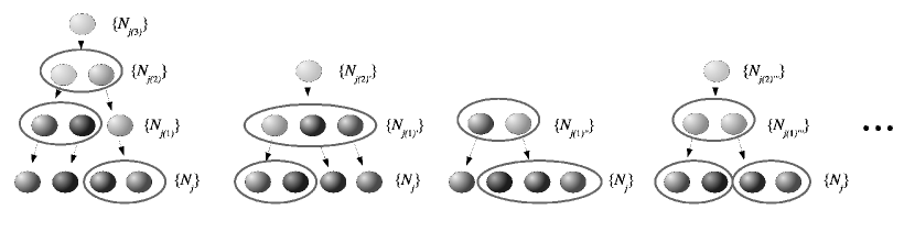
Figure 2: Examples of possible decay trees for a four particles channel. Circles encompass decay products of the particle at higher level.

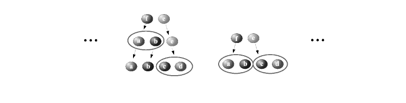
Figure 3: Examples of possible equivalent decay trees for a four particles channel.

Our method is to list all subsets of particles in the channel $\{N_{j}\}$ and check whether there is one or more resonances decaying in each subset. For instance, for a channel with four particles labelled with $1,2,3,4$, possible subsets are:

$$(1)(2,3,4)\qquad\qquad(2,3)(1)(4)$$

$$(2)(1,3,4)\qquad\qquad(2,4)(1)(3)$$

$$(3)(1,2,4)\qquad\qquad(3,4)(1)(2)$$

$$(4)(1,2,3)\qquad\qquad(1,2)(3,4)$$

$$(1,2)(3)(4)\qquad\qquad(1,3)(2,4)$$

$$(1,3)(2)(4)\qquad\qquad(1,4)(2,3)$$

$$(1,4)(2)(3)\qquad\qquad(1,2,3,4)\;.$$

Each resonance decaying into a subset gives rise to a possible upper-level parent channel made of the resonance replacing the given subset and the remaining hadrons of the original channel. For each parent channel found, the procedure is iterated. At the uppermost level, possibly one has a channel with only one massive resonance having the same quantum numbers as the initial state.

The complexity of this combinatorial problem is considerable. Actually, the number $B_{n}$ of subsets of a set of $n$ integers is known as the Bell number which is given in terms of a recurrence relation:

$$B_{n+1}=\sum_{k=0}^{n}B_{k}{n\choose k}\;.$$ (49)

This number grows quickly as a function of $n$, so that listing all possible parent channels becomes practically impossible for channels with more than $\sim 8$ particles ($B_{8}=4140$ and $B_{9}=21147$), also in view of the very large number of resonances in the hadron spectrum.

Indeed, this recursive search algorithm can give rise to multiple counting. This happens if there are identical particles in the channel simply because some subsets are actually the same. For instance, if there are four particles, the subsets $(1,2)(3,4)$ and $(1,3)(2,4)$ are clearly equivalent if particles $2$ and $3$ are identical. This kind of double counting is quite easy to get round algorithmically a priori. Yet, double counting may occur even if particles in the channel are all different. Consider for instance two decay trees like those shown in fig. 3 with, on the left, the subset $(a)(b)(cd)$ and on the right the subset $(ab)(cd)$. In fact, both configurations can stem from the same channel $e,f$ at a different level, so this parent channel may appear twice in our parent channel search. This kind of multiple counting is avoided by re-checking a posteriori the full list of parent channels found.

Finally, the probability $\rho_{\{N_{j}\}}$ of observing a final channel $\{N_{j}\}$ can be written as a finite sum over all parent channels:

$$\rho_{\{N_{j}\}} \propto \tilde{\Omega}_{\{N_{j}\}}\equiv\Omega_{\{N_{j}\}}+{\rm BR}_{(1)}\Omega_{\{N_{j}\}_{(1)}}+{\rm BR}_{(2)}{\rm BR}_{(1)}\Omega_{\{N_{j}\}_{(2)}}+\ldots$$ (50)

$$+ {\rm BR}_{(1)^{\prime}}\Omega_{\{N_{j}\}_{(1)^{\prime}}}+{\rm BR}_{(2)^{\prime}}{\rm BR}_{(1)^{\prime}}\Omega_{\{N_{j}\}_{(2)^{\prime}}}+\ldots$$

where ${\rm BR}_{(i)}$ is the product of branching ratios of particles in the channel $\{N_{j}\}_{(i)}$ decaying into particles in the channel $\{N_{j}\}_{(i-1)}$ and where $\tilde{\Omega}_{\{N_{j}\}}$ is, by definition, the total channel weight, including contributions of parent channels.

V Analysis of $\textrm{e}^{+}\textrm{e}^{-}$ collisions at low energy

As has been mentioned in the Introduction, the rates of exclusive hadronic channels can be measured only in low energy collisions (say $\lesssim 5$ GeV) because the large multiplicity of the final state at high energy makes a full identification of particles impossible. There have been in the past some attempts to reproduce hadron multiplicities and some multi-pion(kaon) differential cross sections in low energy $\textrm{e}^{+}\textrm{e}^{-}$ collisions eestat2 by using statistical-thermodinamical or statistical-inspired models. Yet, in none of those calculations the full set of conservation laws has been taken into account, because of the lack of a proper formulation of the microcanonical ensemble with intrinsic angular momentum and the involved numerical calculations. As we will show in Subsect. V.1, this is a serious drawback because, when dealing with exclusive channels, all conservation laws play a major role. In fact, we now have all needed ingredients to make a proper test of the statistical hadronization model with exclusive channels: the statistical weight of multi-particle channels including exact energy-momentum and intrinsic angular momentum conservation bf4 (formula (34) and a sufficient computing power.

As discussed in Sect. II, at low energy the formation of a single cluster at rest in the centre-of-mass frame of an $\textrm{e}^{+}\textrm{e}^{-}$ collision is assumed. Its mass will therefore coincide with $\sqrt{s}$ and the other quantum numbers will be those of the initial state. Particularly, in $\textrm{e}^{+}\textrm{e}^{-}$ collision, the hadron production is dominated by the diagram with an intermediate virtual photon (see fig. 1), so that the hadronizing cluster is assigned with a spin, parity and C-parity $J^{PC}=1^{--}$. On the other hand, isospin is not conserved in electromagnetic interaction and it is therefore unknown; in the Vector Dominance Model (VDM) this depends on the coupling of the photon to different resonances, but we will be working in a mass region above 2 GeV, far from known resonance region (see discussion in the following). Therefore, we will assume an unknown statistical mixture of $I=0$ and $I=1$ initial state, neglecting interference terms, and introducing a free parameter ${\rm I}_{0}$ such that for the mixed state:

$${\rm I}_{0}|0,0\rangle\langle 0,0|+(1-{\rm I}_{0})|1,0\rangle\langle 1,0|,$$

Finally, the geometry of the cluster needs to be fixed. We assume a spherical shape and a volume given by:

$$V=\frac{M}{\rho}=\frac{\sqrt{s}}{\rho}$$ (51)

where $M$ is the mass and $\rho$ the energy density; this is taken to be a free parameter to be determined by comparing the model with the data.

Motivated by observations concerning hadron abundances at high energy, we allow deviation from the full statistical equilibrium of channels involving particles with strange valence quarks. This is done by introducing in the analysis the extra-strangeness suppression parameter $\gamma_{S}$ rafelski . For its definition here to be in agreement with the formulae of inclusive multiplicities of hadrons in the canonical and grand-canonical ensembles, one just needs to multiply the microcanonical weight of a channel by $\gamma_{S}^{s_{j}}$, $s_{j}$ being the number of valence strange quarks of each particle:

$$\Omega_{\{N_{j}\}}\rightarrow\left[\prod_{j=1}^{K}\left(\gamma_{S}^{s_{j}}\right)^{N_{j}}\right]\Omega_{\{N_{j}\}}$$ (52)

The $\gamma_{S}$ factor also applies to neutral mesons with hidden strange quark content like $\eta$, $\phi$ etc. Since the wavefunction of such particles is in general a superposition like $C_{{\rm u}}{\rm u}\overline{{\rm u}}+C_{{\rm d}}{\rm d}\overline{{\rm d}}+C_{{\rm s}}{\rm s}\overline{{\rm s}}$ with $|C_{{\rm u}}|^{2}+|C_{{\rm d}}|^{2}+|C_{{\rm s}}|^{2}=1$, only the component ${\rm s}\overline{{\rm s}}$ of the wavefunction is suppressed, i.e. we multiply by:

$$\left[|C_{{\rm s}}|^{2}\gamma_{S}^{2}+(1-|C_{{\rm s}}|^{2})\right]\;.$$

for each neutral meson. To calculate $|C_{{\rm s}}|^{2}$, we have used mixing angles quoted by the Particle Data Book pdg2010 .

The branching ratios, masses and widths of hadrons and resonances needed to calculate the exclusive channel rate according to formula (50), have also been taken from the latest issue of the Particle Data Book pdg2010 . All hadrons up to a mass of 1.8 GeV for mesons and 1.9 for baryons have been included for the generation of parent channels. It is now appropriate to briefly discuss the possible contribution of single resonance decay (off-peak) to the hadron production in $\textrm{e}^{+}\textrm{e}^{-}$ collisions at low energy. In terms of the diagrammatic description in fig. (2), these contributions correspond to the highest ancestor of the channel in the decay tree, being a single resonance with the same quantum numbers as the initial state. This contribution, if relevant, cannot be subtracted away from the experimental data given the poor knowledge of resonances above 1.8-1.9 GeV mass. If one assumes that resonances can be identified with clusters decaying statistically, then this contribution should be somehow taken into account within the SHM calculation itself. On the other hand, if we refrain from this assumption, we must move sufficiently far from the energy region where narrow resonances lie in order to minimize their impact on the cross section. Furthermore, we do not want to get over the charm quark production threshold and this constrains the energy interval to about 2-3 GeV.

$\sqrt{s}$ (GeV)	$\rho$ (GeV/fm3)	$\gamma_{S}$	$C_{\rho\gamma_{S}}$ (GeV/fm3)	I0	A (nb GeV4)	$\chi^{2}$/dof
$2.1$	$0.24\pm 0.17$	$0.66\pm 0.22$	$0.011$	$0.17\pm 0.03$	$0.028\pm 0.002$	93.4/16
$2.2$	$0.36\pm 0.20$	$0.86\pm 0.22$	$0.023$	$0.15\pm 0.03$	$0.036\pm 0.002$	82.6/14
$2.4$	$0.44\pm 0.30$	$0.78\pm 0.36$	$0.024$	$0.23\pm 0.04$	$0.017\pm 0.001$	55.4/17
$2.6$	$0.56\pm 0.36$	$0.62\pm 0.47$	$-0.009$	$0.53\pm 0.07$	$0.017\pm 0.002$	44.9/12

Table 1: Summary of the fit results to multi-hadronic exclusive channels at different centre-of-mass energies. Also shown the correlation coefficient of $\rho$ and $\gamma_{S}$.

Figure 4: Upper panel: best fit energy density $\rho$ as a function of centre-of-mass energy. Lower panel: best fit $\gamma_{S}$ values. Lines are drawn to guide the eye.

Much data in this energy interval has been lately provided by the BABAR experiment which has measured the cross-sections of several multi-hadronic channels in $\textrm{e}^{+}\textrm{e}^{-}$ collisions at several centre-of-mass energies with the method of initial state radiation. We have chosen four energy points, that is $\sqrt{s}=$ 2.1, 2.2, 2.4 and 2.6 GeV and added to the available BABAR measurements older measurements performed by experiments at $\textrm{e}^{+}\textrm{e}^{-}$ colliders run at the same centre-of-mass energies and collected in a nice review paper Whalley:2003qr . In fact, most centre-of-mass energies were near, but not exactly, those values. Therefore, for each chosen energy, we have interpolated cross sections by making a simple mean of cross sections and errors measured at adjacent energy values. For each energy point, the thereby obtained cross-section values and errors from different experiments have been further averaged according to the weigthed average method used by the Particle Data Group pdg2010 , including error rescaling by $\chi^{2}/dof$ in case of large discrepancy. The full set of channels can be read through in tables 2, 3, 4, 5 in Appendix C.

In order to compare the calculation with the data of exclusive channels rate, given in terms of a cross section, we have introduced a normalization free parameter $A(\sqrt{s})$:

$$\sigma_{\{N_{j}\}}=A(\sqrt{s})\omega_{\{N_{j}\}}$$ (53)

Finally, we have fitted all available measurements of exclusive channels rates at a given energy to the SHM with four free parameters: $\rho$, $\gamma_{S}$, $A$ and $I_{0}$. The fit minimizes the $\chi^{2}$:

$$\chi^{2}=\sum_{\{N_{j}\}_{\rm measured}}\frac{\left(\sigma_{\{N_{j}\}}^{\rm exp}-\sigma_{\{N_{j}\}}^{\rm theo}\right)^{2}}{\Delta^{2}_{\rm exp}+\Delta^{2}_{\rm theo}}\;.$$ (54)

where the sum runs over measured channels; $\Delta_{\rm exp}$ is the experimental error and $\Delta_{\rm theo}$ is the theoretical uncertainty on the cross sections respectively. The latter is the sum in quadrature of the statistical error, owing to the finite statistics in Monte-Carlo integration and the systematic error stemming from the uncertainty on branching ratios of resonances. This error has been estimated at each step of the $\chi^{2}$ minimization by varying the branching ratios by their errors quoted in the Particle Data Book (or by making an educated guess if missing) and calculating the difference between the theoretical value of the probability (50) before and after the variation. This additional uncertainty generally overcomes the experimental error for ligth particle channels with $>2$ particles, as the number of contributing channels with resonances is large (as it can be seen in tables 2, 3, 4 and 5 in Appendix C).

The fit procedure is as follows: for each energy point a two-dimensional grid in the parameters $\rho$ and $\gamma_{S}$ is set, with 50 divisions in each direction and range [0.04-2] GeV/fm³, [0.02-1] respectively. At each point of the grid, a minimization of the $\chi^{2}$ is carried out to determine the parameters $I_{0}$ and $A$. The point grid where the minimum among all minima lies has been taken as the best fit. The error on the parameters $\rho$ and $\gamma_{S}$ has been estimated graphically from the contour $\chi^{2}=\chi^{2}_{\rm min}+1$ (see fig. 5).

Figure 5: Contour plot of the $\chi^{2}$ for $\sqrt{s}=2.4\;$ GeV.

The fit results are shown in summarized in table 1 and in fig. 4. The comparison of the fitted rates with the data is shown in figs. 8, 9, 10, 11 and in tables 2, 3, 4, 5 in Appendix C for $\sqrt{s}=$ 2.1, 2.2, 2.4, 2.6 GeV respectively.

Figure 6: Fits to exclusive channels in $\textrm{e}^{+}\textrm{e}^{-}$ collisions at 2.4 with conservation laws turned off. The data points, shown as full dots, are weighted averages of available measurements (see text) while the fitted points are shown as open squares. Panel (a): fit with only energy-momentum conservation. Panel (b): fit without angular momentum conservation.

V.1 Test of conservation laws

To appraise the role of the various constraints and the features of the statistical model, it is worth making the fit by switching off the conservation laws in turn. We have therefore minimized the $\chi^{2}$ with the same aforementioned procedure, at a single energy point $\sqrt{s}=$ 2.4 GeV, in two different modes.

In the first mode we have kept only the conservation of energy and momentum, disregarding angular momentum, parity and internal symmetries. The result is shown in fig. 6, where a consistent worsening of the fit quality can be seen ($\chi^{2}$/dof = 133/17), especially looking at the residual distribution. The fit quality significantly improves by turning on the internal symmetries ($\chi^{2}$/dof = 74.5/17). Finally, restoring the angular momentum and parity conservation, one obtains the best fit shown in fig. 10 ($\chi^{2}$/dof = 55.4/17). This further improvement indicates that angular momentum conservation plays an important role and this was indeed expected as this is a very effective mechanism in modulating the rate of a channel for a spacially extended source (the well known centrifugal barrier effect), which is one of the crucial assumption of the statistical model.

Figure 7: Normalized microcanonical weights of the channel $\pi^{0}\pi^{0}$ as a function of the cluster spin $J$ in the Boltzmann statistics (upper panel) and quantum statistics (lower panel) case. The cluster has been taken spherical in shape with radius $R=4$ GeV^-1 and a mass $M=5$ GeV. Isospin, parity, $C$-parity conservation are turned off.

To highlight this effect, we have calculated the microcanonical channel weight for the channel $\pi^{0}\pi^{0}$ for different spin $J$ of the cluster. Assuming a spherical shape and switching off parity and internal symmetries (isospin and charge conjugation) we have obtained the normalized microcanonical channel weights shown in fig. (7), for a cluster mass $M$ of $5$ GeV and a radius of $R=4$ GeV^-1. As expected, the maximal value of the microcanonical channel weight is located around the angular momentum $J\sim{\rm p}R\sim 10$, $\rm p$ being the momentum of the pion. This calculation also served as a consistency check for our numerical code as the sum of all microcanonical channel weights for all $J$ was found to reproduce the simple two-body phase space with only energy-momentum conservation.

Figure 8: Upper panel: exclusive cross sections of various channel in $\textrm{e}^{+}\textrm{e}^{-}$ collisions at 2.1 GeV. The data points, shown as full dots, are weighted averages of available measurements (see text) while the fitted points are shown as open squares. The lines have been drawn to guide the eye. Lower panel: fit residual distribution.

Figure 9: Upper panel: exclusive cross sections of various channel in $\textrm{e}^{+}\textrm{e}^{-}$ collisions at 2.2 GeV. The data points, shown as full dots, are weighted averages of available measurements (see text) while the fitted points are shown as open squares. The lines have been drawn to guide the eye. Lower panel: fit residual distribution.

Figure 10: Upper panel: exclusive cross sections of various channel in $\textrm{e}^{+}\textrm{e}^{-}$ collisions at 2.4 GeV. The data points, shown as full dots, are weighted averages of available measurements (see text) while the fitted points are shown as open squares. The lines have been drawn to guide the eye. Lower panel: fit residual distribution.

Figure 11: Upper panel: exclusive cross sections of various channel in $\textrm{e}^{+}\textrm{e}^{-}$ collisions at 2.6 GeV. The data points, shown as full dots, are weighted averages of available measurements (see text) while the fitted points are shown as open squares. The lines have been drawn to guide the eye. Lower panel: fit residual distribution.

VI Discussion and conclusions

Although the fit quality is not perfect in terms of statistical test (see table 1), we can fairly conclude, looking at figs. 8, 9, 10, 11 that the statistical hadronization model is able to satisfactorilty reproduce most exclusive multi-hadronic channels measured in $\textrm{e}^{+}\textrm{e}^{-}$ collisions at low energy. Especially at 2.4 GeV, all measured channel rates lie within 2.5 standard deviations from the model values, which is quite remarkable taking into account the obvious fact that exclusive channels are a very stringent test for any model, certainly much more than inclusive multiplicities, and that the fits were done with only 4 free parameters.

To fairly judge the quality of the agreement between model and data, it is worth keeping in mind that the analysis we have presented in this work still relies on several approximations, so that one may hope that a more thorough calculation will result in a better agreement between model and data. The main approximation introduced in this calculation is the assumption of validity of the hadron-resonance gas model for exclusive channels and at finite volume, what is in fact granted only for fully inclusive quantities and in the thermodynamic limit. Moreover, the assumed symmetry SU(2)${}_{\rm iso}\otimes$U(1)_strange may not be a sufficiently realistic scheme.

The statistical model nicely matches one of the main features of the data, namely the gross dependence of the channel rate on the number of particles $N$; this kind of hyerarchy can be clearly observed in all fits (see e.g. fig. 10) and the SHM is able to reproduce this behaviour because of the approximate dependence of the rate on $V^{N}$, as in formula (18). Furthermore, the more conservation laws are included, the more the fit improves and the more the model predictions approach the actual rates. This is a certainly a good point for the SHM, especially as far as angular momentum is concerned, as has been discussed in Subsect. V.1.

Overall, the most interesting outcome of the analysis are the values of the fitted energy density $\rho$ and strangeness suppression parameter $\gamma_{S}$, shown in fig. 4, around 0.5 GeV/fm³ and 0.7 respectively. These values are essentially the same obtained with the analysis of inclusive hadronic multiplicities at high energy review and this confirms the consistency of the statistical approach to hadronization. While the origin of extra-strangeness suppression is not clear (an interesting proposal was put forward in ref. bcms ) the idea of hadronization as a process occurring at a critical energy density which uniformly populates the available phase space is certainly reinforced by the observation that this seems to happen at universal values of the parameters, at high as well as at low energy.

The interpretation of the statistical equilibrium in hadronization is an open issue and there are several proposals. One of the authors (F.B.) favours the idea of a quantum-chaotic effect (known as Berry’s conjecture) owing the the strong non- linearity of QCD in the non-perturbative regime.

References

J. D. Bjorken and S. J. Brodsky, Phys. Rev.  D 1 (1970) 1416; J. Engels, K. Schilling and H. Satz, Nuovo Cim.  A 17 (1973) 535; C. E. Carlson and F. Gross, Phys. Rev.  D 14 (1976) 1858.

G. Eilam, C. Hojvat, B. Margolis, W. J. Meggs, S. C. Frautschi and M. Pripstein, Lett. Nuovo Cim.  14 (1975) 108; B. Margolis, W. J. Meggs and N. Weiss, Phys. Rev.  D 13 (1976) 2551; S. Rudaz, Lett. Nuovo Cim.  6S2 (1973) 292, Lett. Nuovo Cim.  6 (1973) 292.

F. Becattini, Introduction to the statistical hadronization model, arXiv:0901.3643; F. Becattini, R. Fries in Relativistic heavy ion physics, Landolt-Börnstein 1-23 (2010), arXiv:0907.1031.

F. Becattini, Z. Phys.  C 69 (1996) 485 ; F. Becattini and U. W. Heinz, Z. Phys.  C 76 (1997) 269 ; F. Becattini and G. Passaleva, Eur. Phys. J.  C 23 (2002) 551 ; F. Becattini, P. Castorina, J. Manninen and H. Satz, Eur. Phys. J. C 56, (2008) 493 ; F. Becattini, P. Castorina, A. Milov and H. Satz, Eur. Phys. J.  C 66 (2010) 377 ; I. Kraus, J. Cleymans, H. Oeschler and K. Redlich, Phys. Rev. C 79, (2009) 014901 ; I. Kraus, J. Cleymans, H. Oeschler and K. Redlich, Phys. Rev.  C 81, (2010) 024903 ; A. Andronic et al., Phys. Lett.  B 678, (2009) 350 .

J. Cleymans, H. Satz, Z. Phys.  C 57 (1993) 135 ; P. Braun-Munzinger, J. Stachel, J. P. Wessels and N. Xu, Phys. Lett.  B 365 (1996) 1 ; F. Becattini, M. Gazdzicki and J. Sollfrank, Eur. Phys. J.  C 5 (1998) 143 ; P. Braun-Munzinger, D. Magestro, K. Redlich and J. Stachel, Phys. Lett.  B 518, (2001) 41; A. Baran, W. Broniowski and W. Florkowski, Acta Phys. Polon.  B 35 (2004) 779; J. Cleymans, B. Kampfer, M. Kaneta, S. Wheaton and N. Xu, Phys. Rev.  C 71 (2005) 054901; F. Becattini, M. Gazdzicki, A. Keranen, J. Manninen and R. Stock, Phys. Rev.  C 69 (2004) 024905.

F. Becattini and G. Passaleva, Eur. Phys. J.  C 23 (2002) 551 .

U. Heinz, Nucl. Phys. A 661 (1999) 140; R. Stock, Phys. Lett. B 456 (1999) 277; A. Bialas, Phys. Lett. B 466 (1999) 301; H. Satz, Nucl. Phys. Proc. Suppl. 94 (2001) 204; J. Hormuzdiar,S. D. H. Hsu, G. Mahlon Int. J. Mod. Phys. E 12 (2003) 649; V. Koch, Nucl. Phys. A 715 (2003) 108 ;
L. McLerran, arXiv:hep-ph/0311028;
Y. Dokshitzer, Acta Phys. Polon. B 36 (2005) 361; H. Satz, AIP Conf. Proc.  1038 (2008) 225 ; Eur. Phys. J. ST 155 (2008) 167 ; D. Kharzeev, Nucl. Phys. A 774 (2006) 315; F. Becattini, J. Phys. Conf. Ser. 5 (2005) 175; F. Becattini, arXiv:0901.3643 (2009); F. Becattini, R. Fries in Relativistic heavy ion physics, Landolt-Börnstein 1-23 (2010), arXiv:0907.1031.

R. Hagedorn, CERN lectures Thermodynamics of strong interactions (1970); R. Hagedorn in Hot hadronic matter (New York: Plenum Press), preprint CERN-TH 7190/94 (1994).

F. Becattini, J. Phys. Conf. Ser. 5 (2005) 175.

W. Blumel, P. Koch and U. W. Heinz, Z. Phys.  C 63 (1994) 637.

F. Becattini and L. Ferroni, Eur. Phys. J.  C 51 (2007) 899.

F. Becattini and L. Ferroni, Eur. Phys. J.  C 52 (2007) 597.

F. Becattini and L. Ferroni, Eur. Phys. J.  C 38 (2004) 225. [Erratum-ibid.  66, 341 (2010)].

F. Becattini and L. Ferroni, Eur. Phys. J.  C 35 (2004) 243.

R. Dashen, S. K. Ma and H. J. Bernstein, Phys. Rev.  187 (1969) 345.

F. Cerulus, N. Cim. X22 (1961) 958-995.

T. Gabbriellini Studio di un generatore di eventi per il modello statistico di adronizzazione, University of Florence (2004) Diploma thesis (in Italian).

R. H. C. Cheng, Communications of the ACM 21 (1978) 317.

J. Rafelski, Phys. Lett. B 262 (1991) 333.

K. Nakamura et al. (Particle Data Group), J. Phys. G 37 (2010) 075021.

M. R. Whalley, J. Phys. G 29 (2003) A1.

F. Becattini, P. Castorina, J. Manninen and H. Satz, Eur. Phys. J. C 56 (2008) 493.

F. Cerulus, Suppl. N. Cim. X5 (1960) 402.

B. Aubert et al. [BABAR Collaboration], Phys. Rev. Lett.  103 (2009) 231801 [arXiv:0908.3589 [hep-ex]].

B. Aubert et al. [BABAR Collaboration], Phys. Rev.  D 70 (2004) 072004 [arXiv:hep-ex/0408078].

B. Aubert et al. [BABAR Collaboration], Phys. Rev.  D 71 (2005) 052001 [arXiv:hep-ex/0502025].

B. Aubert et al. [BABAR Collaboration], Phys. Rev.  D 76 (2007) 092005 [Erratum-ibid.  D 77 (2008) 119902]

B. Aubert et al. [BABAR Collaboration], Phys. Rev.  D 76 (2007) 012008 [arXiv:0704.0630 [hep-ex]].

B. Aubert et al. [BaBar Collaboration], Phys. Rev.  D 77 (2008) 092002 [arXiv:0710.4451 [hep-ex]].

B. Aubert et al. [BABAR Collaboration], Phys. Rev.  D 76 (2007) 092006 [arXiv:0709.1988 [hep-ex]].

Appendix A

The charge-conjugation operator ${\sf C}$, when acting on a charged light-flavoured meson belonging to an isotriplet may generate an arbitrary phase. Fixing this phase is essential for our definition of the projector (23). For this purpose, let us define the operator $\widehat{{\sf G}}$ as:

$$\widehat{{\sf G}}=\widehat{{\sf C}}\;{\rm e}^{i\pi\widehat{I}_{2}}$$ (55)

which is known as G-parity operator. When applied to a state with third component of isospin $I_{3}$, this amounts to first flipping $I_{3}\rightarrow-I_{3}$ and reversing the process, $-I_{3}\rightarrow I_{3}$. Therefore, an eigenvector of $\widehat{\sf I}_{3}$ is also an eigenvector of the G-parity operator. For an isotriplet like pions’:

$$\widehat{{\sf G}}|\pi^{\pm}\rangle=-\widehat{\sf C}|\pi^{\pm}\rangle$$ (56)

$$\widehat{{\sf G}}|\pi^{0}\rangle=\pm|\pi^{0}\rangle\;.$$

because ${\rm e}^{i\pi\widehat{I}_{2}}$ results in a factor $-1$ when applied to any pion state. Now, since $|\pi^{0}\rangle$ is an eigenstate of $\widehat{\sf C}$ with eigenvalue $+1$, we define:

$$\widehat{{\sf C}}|\pi^{\pm}\rangle=-|\pi^{\mp}\rangle\;.$$ (57)

so as to G-parity to yield the same eigenvalue for all members of the isotriplet.

Appendix B

One of the important steps in the numerical evaluation of the microcanonical channel weight is the computation of:

$$\mathcal{I}_{\boldsymbol{\rho}}^{\{N_{j}\}}\left(I,I_{3}\right)\equiv\left[\prod_{j=1}^{K}\langle I_{j},\{I_{3}^{n_{j}}\}|\right]|I,I_{3}\rangle\langle I,I_{3}|\left[\prod_{j=1}^{K}|\{I_{j},I_{3}^{\rho_{j}(n_{j})}\}\rangle\right]$$ (58)

We describe here a method to compute the more general expression:

$$\left\{\langle I^{1},I^{1}_{3}|\langle I^{2},I_{3}^{2}|\cdots\langle I^{N},I_{3}^{N}|\right\}|I,I_{3}\rangle\langle I,I_{3}|\left\{|I^{1},I_{3}^{1}\,{}^{\prime}\rangle|I^{2},I_{3}^{2}\,{}^{\prime}\rangle\cdots|I^{N},I_{3}^{N}\,{}^{\prime}\rangle\right\}\qquad$$ (59)

where

$$|I^{1},I_{3}^{1}\rangle|I^{2},I_{3}^{2}\rangle\cdots|I^{N},I_{3}^{N}\rangle$$ (60)

is a generic multi-particle isospin state. A closed analytical formula for (58), as a finite sum, has been found in ref. ceriso4 . We have not used that formula, yet, in the following, we will closely follow the notations therein.

In order to calculate the projection of the state (60) onto the subspace with total isospin $|II_{3}\rangle$, one should use a system of base-vectors in isospin space where $I$ is diagonal. The choice of such a basis is equivalent to the choice of a coupling scheme for the $I_{i}$ ceriso4 ; we can choose, for instance, a base where:

$$(I^{12})^{2}=(I^{1}+I^{2})^{2}$$ (61)

$$(I^{123})^{2}=(I^{1}+I^{2}+I^{3})^{2}$$

$$\ldots$$

are diagonal.

A base vector for this scheme is denoted by:

$$|I^{12},I^{123},\ldots,I,I_{3}\rangle$$ (62)

where $I^{1}$, $I^{2}$, etc., are known. Both sets (62) and (60) are complete and they are connected by a unitary transformation:

$$|I^{12},I^{123},\ldots,I,I_{3}\rangle$$ (63)

$$=\sum_{I_{3}^{1},\ldots,I_{3}^{N}}\left\{\langle I^{1},I_{3}^{1}|\cdots\langle I^{N},I_{3}^{N}|\right\}|I^{12},I^{123},\ldots,I,I_{3}\rangle\left\{|I^{1},I_{3}^{1}\rangle\cdots|I^{N},I_{3}^{N}\rangle\right\}$$

The coefficient $\left\{\langle I^{1},I_{3}^{1}|\cdots\langle I^{N},I_{3}^{N}|\right\}|I^{12},I^{123},\ldots,I,I_{3}\rangle$ is called a recoupling coefficient and is a product of Clebsch-Gordan coefficients:

$$\left\{\langle I^{1},I_{3}^{1}|\cdots\langle I^{N},I_{3}^{N}|\right\}|I^{12},I^{123},\ldots,I,I_{3}\rangle=C^{I^{1}I^{2}I^{12}}_{I_{3}^{1}I_{3}^{2}(I_{3}^{1}+I_{3}^{2})}\cdots C^{I^{12\ldots N-1}I^{N}I}_{(I_{3}^{1}+I_{3}^{2}+\ldots I_{3}^{N-1})I_{3}^{N}I_{3}}\qquad$$ (64)

By using eq. (64) one can rewrite (59) as:

$$\left\{\langle I^{1},I^{1}_{3}|\cdots\langle I^{N},I_{3}^{N}|\right\}|I,I_{3}\rangle\langle I,I_{3}|\left\{|I^{1},I_{3}^{1}\,{}^{\prime}\rangle\cdots|I^{N},I_{3}^{N}\,{}^{\prime}\rangle\right\}$$ (65)

$$\qquad=\sum_{I^{12}I^{123}\ldots I^{12\ldots N-1}}\left\{\langle I^{1},I_{3}^{1}|\cdots\langle I^{N},I_{3}^{N}|\right\}|I^{12},I^{123},\ldots,I,I_{3}\rangle$$

$$\qquad\times\langle I^{12},I^{123},\ldots,I,I_{3}|\left\{|I^{1},I_{3}^{1}\,{}^{\prime}\rangle\cdots|I^{N},I_{3}^{N}\,{}^{\prime}\rangle\right\}$$

$$\qquad=\sum_{I^{12}I^{123}\ldots I^{12\ldots N-1}}C^{I^{1}I^{2}I^{12}}_{I_{3}^{1}I_{3}^{2}(I_{3}^{1}+I_{3}^{2})}\cdots C^{I^{12\ldots N-1}I^{N}I}_{(I_{3}^{1}+I_{3}^{2}+\ldots I_{3}^{N-1})I_{3}^{N}I_{3}}$$

$$\qquad\times C^{I^{1}I^{2}I^{12}}_{I_{3}^{1}\,{}^{\prime}I_{3}^{2}\,{}^{\prime}(I_{3}^{1}\,{}^{\prime}+I_{3}^{2}\,{}^{\prime})}\cdots C^{I^{12\ldots N-1}I^{N}I}_{(I_{3}^{1}\,{}^{\prime}+I_{3}^{2}\,{}^{\prime}+\ldots I_{3}^{N-1}\,{}^{\prime})I_{3}^{N}\,{}^{\prime}I_{3}}$$

of course, if one of the Clebsch-Gordan coefficient is vanishing, the corresponding term in the previous sum is vanishing too.

We have implemented a recursive numerical method to calculate the above expression. By iterating the coupling scheme in (61) one can build a tree diagram, shown in fig. (12) from left to right, where for each recoupling step, the highest value of the resulting isospin is put on top and the other values are sorted in decreasing order.

Figure 12: Tree diagram for the calculation of isospin matrix elements.

To each branch of the tree a numerical coefficient is associated, which is the recursive product of the Clebsch-Gordan coefficient corresponding to the decomposition which generated that branch and the numerical coefficient of the generating branch. At the righmost end of the tree, one finds all possible values of the global isospin which can be obtained by coupling the set $I^{1},I_{3}^{1};\ldots;I^{N},I_{3}^{N}$ and the corresponding recoupling coefficients $\langle I,I_{3}|I^{1},I_{3}^{1},I^{2},I_{3}^{2},\ldots I^{N},I_{3}^{N}\rangle$.

The main advantage of this algorithm resides in the possibility of a simple recursive implementation. Moreover, the CPU time needed for the tree exploration can be easily reduced by simply switching off the recursion for branches with vanishing Clebsch-Gordan coefficients.

Appendix C

In this Appendix we have collected the tables with best fit values and the experimental values of the cross sections of exclusive channels.

$\sqrt{s}=2.1$ GeV
channel	$\sigma_{SHM}$ (nb)	$\sigma_{exp.}$ (nb)	References
$\pi^{+}\pi^{-}$	$0.229\pm 0.003\pm 0$	$0.177\pm 0.036$	:2009fg ; Whalley:2003qr
$\pi^{+}\pi^{-}\pi^{0}$	$0.133\pm 0.002\pm 0.03$	$0.385\pm 0.11$	Whalley:2003qr ; Aubert:2004kj
$\pi^{+}\pi^{-}\pi^{0}\pi^{0}$	$5.93\pm 0.06\pm 0.5$	$6.2\pm 2.57$	Whalley:2003qr
$\pi^{+}\pi^{-}\pi^{+}\pi^{-}$	$3.96\pm 0.02\pm 0.4$	$4.18\pm 0.45^{*}$	Whalley:2003qr ; Aubert:2005eg
$\pi^{+}\pi^{-}\pi^{0}\pi^{0}\pi^{0}$	$0.809\pm 0.02\pm 0.05$	$4.03\pm 2.41$	Whalley:2003qr
$\pi^{+}\pi^{-}\pi^{+}\pi^{-}\pi^{0}$	$1.46\pm 0.01\pm 0.07$	$1.46\pm 0.4^{*}$	Whalley:2003qr ; Aubert:2007ef
$\eta\pi^{+}\pi^{-}$	$0.758\pm 0.02\pm 0.09$	$0.36\pm 0.11$	Whalley:2003qr ; Aubert:2007ef
$\omega\pi^{0}$	$0.261\pm 0.004\pm 0$	$0.68\pm 0.19$	Whalley:2003qr
$K^{+}K^{-}$	$0.0673\pm 0.0007\pm 0$	$0.18\pm 0.11$	Whalley:2003qr
$\omega\pi^{+}\pi^{-}$	$0.478\pm 0.002\pm 0.001$	$0.3\pm 0.09$	Whalley:2003qr ; Aubert:2007ef
$\eta\pi^{+}\pi^{-}\pi^{+}\pi^{-}$	$2.18\pm 0.02\pm 0.7$	$0.915\pm 0.2$	Aubert:2007ef
$K^{+}K^{-}\pi^{0}$	$0.148\pm 0.005\pm 0.0009$	$0.12\pm 0.042$	Whalley:2003qr ; Aubert:2007ur
$K^{+}K^{-}\pi^{0}\pi^{0}$	$0.242\pm 0.002\pm 0.006$	$0.9\pm 0.134$	Aubert:2007ur
$K^{+}K^{-}\pi^{+}\pi^{-}$	$0.929\pm 0.003\pm 0.05$	$3.05\pm 0.5^{*}$	Whalley:2003qr ; Aubert:2007ur
$K^{+}K^{-}\pi^{+}\pi^{-}\pi^{0}$	$0.6\pm 0.006\pm 0.03$	$0.575\pm 0.13$	Aubert:2007ef
$\eta\phi$	$0.0206\pm 0.0002\pm 0$	$0.425\pm 0.17$	Aubert:2007ym
$\omega f_{0}$	$0.151\pm 0.0007\pm 0$	$0.39\pm 0.11$	Aubert:2007ef
$p\overline{p}$	$0.479\pm 0.002\pm 0$	$0.63\pm 0.076$	Whalley:2003qr
$n\overline{n}$	$0.48\pm 0.002\pm 0$	$1\pm 0.28$	Whalley:2003qr
$K^{+}K^{-}K^{+}K^{-}$	$0.0331\pm 6e-05\pm 0$	$0.019\pm 0.007$	Aubert:2007ur
Not included in the fit
$\eta^{\prime}\pi^{+}\pi^{-}$	$0.371\pm 0.005\pm 0.008$	$0.17\pm 0.07^{**}$	Aubert:2007ef
$\phi\pi^{+}\pi^{-}$	$0.127\pm 0.0009\pm 0$	$0.395\pm 0.065^{**}$	Aubert:2007ur
$K^{*}_{0}(892)K^{-}\pi^{+}$	$0.324\pm 0.002\pm 0.01$	$1.07\pm 0.08^{**}$	Aubert:2007ur
$f_{1}\pi^{+}\pi^{-}$	$1.06\pm 0.005\pm 0.2$	$0.79\pm 0.24^{**}$	Aubert:2007ef
$\omega K^{+}K^{-}$	$0.24\pm 0.001\pm 0$	$0.49\pm 0.09^{**}$	Aubert:2007ef
$\phi f_{0}$	$0.089\pm 0.0002\pm 0$	$0.41\pm 0.08^{**}$	Aubert:2007ur
∗ Errors have been rescaled because of discrepancies between different experiments.
∗∗ Errors are statistical only.

Table 2: Comparison between fitted and experimental cross sections of exclusive multi-hadronic channels in $\textrm{e}^{+}\textrm{e}^{-}$ collisions at $\sqrt{s}=$ 2.1 GeV. The errors on theoretical cross sections $\sigma_{SHM}$ are the Monte-Carlo integration statistical error and the error owing to uncertainty on branching ratios of resonances contributing to the channel, respectively. The experimental cross section values have been obtained by averaging available measurements, see text.

$\sqrt{s}=2.2$ GeV
channel	$\sigma_{SHM}$ (nb)	$\sigma_{exp.}$ (nb)	References
$\pi^{+}\pi^{-}$	$0.188\pm 0.002\pm 0$	$0.101\pm 0.0359$	:2009fg
$\pi^{+}\pi^{-}\pi^{0}$	$0.0971\pm 0.003\pm 0.02$	$0.395\pm 0.17$	Aubert:2004kj
$\pi^{+}\pi^{-}\pi^{0}\pi^{0}$	$4.53\pm 0.03\pm 0.4$	$4.2\pm 1.2$	Whalley:2003qr
$\pi^{+}\pi^{-}\pi^{+}\pi^{-}$	$3.34\pm 0.1\pm 0.3$	$3.73\pm 0.2$	Whalley:2003qr ; Aubert:2005eg
$\pi^{+}\pi^{-}\pi^{+}\pi^{-}\pi^{0}$	$1.21\pm 0.01\pm 0.06$	$1.25\pm 0.26$	Aubert:2007ef
$\eta\pi^{+}\pi^{-}$	$0.712\pm 0.007\pm 0.1$	$0.48\pm 0.12$	Aubert:2007ef
$\omega\pi^{0}$	$0.207\pm 0.003\pm 0$	$0.41\pm 0.2$	Whalley:2003qr
$\omega\pi^{+}\pi^{-}$	$0.355\pm 0.002\pm 0.0008$	$0.2\pm 0.09$	Whalley:2003qr ; Aubert:2007ef
$\eta\pi^{+}\pi^{-}\pi^{+}\pi^{-}$	$2.57\pm 0.03\pm 1$	$1.09\pm 0.215$	Aubert:2007ef
$K^{+}K^{-}\pi^{0}$	$0.166\pm 0.02\pm 0.001$	$0.146\pm 0.05$	Aubert:2007ym
$K^{+}K^{-}\pi^{0}\pi^{0}$	$0.34\pm 0.002\pm 0.008$	$0.57\pm 0.1$	Aubert:2007ur
$K^{+}K^{-}\pi^{+}\pi^{-}$	$1.29\pm 0.005\pm 0.06$	$2.07\pm 0.16$	Whalley:2003qr ; Aubert:2007ur
$K^{+}K^{-}\pi^{+}\pi^{-}\pi^{0}$	$1.34\pm 0.008\pm 0.07$	$0.54\pm 0.13$	Aubert:2007ef
$\eta\phi$	$0.0285\pm 0.0003\pm 0$	$0.235\pm 0.126$	Aubert:2007ym
$\omega f_{0}$	$0.0976\pm 0.0004\pm 0$	$0.17\pm 0.091$	Aubert:2007ef
$K^{+}K^{-}\eta\pi^{+}\pi^{-}$	$0.0134\pm 0.0003\pm 0$	$0.02\pm 0.02$	Aubert:2007ef
$p\overline{p}$	$0.34\pm 0.001\pm 0$	$0.454\pm 0.052$	Whalley:2003qr
$K^{+}K^{-}K^{+}K^{-}$	$0.0648\pm 0.0003\pm 0$	$0.0635\pm 0.015$	Aubert:2007ur
Not included in the fit
$\eta^{\prime}\pi^{+}\pi^{-}$	$0.341\pm 0.005\pm 0.007$	$0.101\pm 0.052^{*}$	Aubert:2007ef
$\phi\pi^{+}\pi^{-}$	$0.139\pm 0.001\pm 0$	$0.27\pm 0.055^{*}$	Aubert:2007ur
$K^{*}_{0}(892)K^{-}\pi^{+}$	$0.508\pm 0.003\pm 0.02$	$0.62\pm 0.062^{*}$	Aubert:2007ur
$f_{1}\pi^{+}\pi^{-}$	$1.02\pm 0.005\pm 0.17$	$0.915\pm 0.24^{*}$	Aubert:2007ef
$\omega K^{+}K^{-}$	$0.3\pm 0.002\pm 0$	$0.39\pm 0.08^{*}$	Aubert:2007ef
$\phi f_{0}$	$0.087\pm 0.0003\pm 0$	$0.295\pm 0.065^{*}$	Aubert:2007ur
∗ Errors are statistical only.

Table 3: Comparison between fitted and experimental cross sections of exclusive multi-hadronic channels in $\textrm{e}^{+}\textrm{e}^{-}$ collisions at $\sqrt{s}=$ 2.2 GeV. The errors on theoretical cross sections $\sigma_{SHM}$ are the Monte-Carlo integration statistical error and the error owing to uncertainty on branching ratios of resonances contributing to the channel, respectively. The experimental cross section values have been obtained by averaging available measurements, see text.

$\sqrt{s}=2.4$ GeV
channel	$\sigma_{SHM}$ (nb)	$\sigma_{exp.}$ (nb)	References
$\pi^{+}\pi^{-}$	$0.0716\pm 0.0009\pm 0$	$0.105\pm 0.0323$	:2009fg
$\pi^{+}\pi^{-}\pi^{0}$	$0.0611\pm 0.001\pm 0.01$	$0.26\pm 0.13$	Aubert:2004kj
$\pi^{+}\pi^{-}\pi^{0}\pi^{0}$	$2.25\pm 0.03\pm 0.4$	$2.7\pm 1$	Whalley:2003qr
$\pi^{+}\pi^{-}\pi^{+}\pi^{-}$	$1.68\pm 0.02\pm 0.3$	$2.12\pm 0.2$	Aubert:2005eg
$\pi^{+}\pi^{-}\pi^{+}\pi^{-}\pi^{0}$	$1.1\pm 0.009\pm 0.1$	$0.975\pm 0.23$	Aubert:2007ef
$\eta\pi^{+}\pi^{-}$	$0.289\pm 0.01\pm 0.06$	$0.145\pm 0.06$	Whalley:2003qr ; Aubert:2007ef
$\omega\pi^{0}$	$0.0785\pm 0.001\pm 0$	$0.38\pm 0.2$	Whalley:2003qr
$\omega\pi^{+}\pi^{-}$	$0.294\pm 0.002\pm 0.04$	$0.09\pm 0.09$	Whalley:2003qr ; Aubert:2007ef
$\eta\pi^{+}\pi^{-}\pi^{+}\pi^{-}$	$1.64\pm 0.02\pm 0.6$	$0.865\pm 0.19$	Aubert:2007ef
$K^{+}K^{-}\pi^{0}$	$0.0739\pm 0.001\pm 0.0009$	$0.111\pm 0.036$	Aubert:2007ym
$K^{+}K^{-}\pi^{0}\pi^{0}$	$0.188\pm 0.002\pm 0.007$	$0.335\pm 0.07$	Aubert:2007ur
$K^{+}K^{-}\pi^{+}\pi^{-}$	$0.912\pm 0.004\pm 0.1$	$1.3\pm 0.167^{*}$	Whalley:2003qr ; Aubert:2007ur
$K^{+}K^{-}\pi^{+}\pi^{-}\pi^{0}$	$1.39\pm 0.006\pm 0.2$	$0.785\pm 0.15$	Aubert:2007ef
$\eta\phi$	$0.0127\pm 0.0002\pm 0$	$0.06\pm 0.0534$	Aubert:2007ym
$\omega f_{0}$	$0.0558\pm 0.0003\pm 0$	$0.06\pm 0.05$	Aubert:2007ef
$K^{+}K^{-}\eta\pi^{+}\pi^{-}$	$0.0604\pm 0.0007\pm 0.01$	$0.025\pm 0.05$	Aubert:2007ef
$p\overline{p}$	$0.129\pm 0.0005\pm 0$	$0.146\pm 0.03$	Whalley:2003qr
$n\overline{n}$	$0.128\pm 0.0005\pm 0$	$0.69\pm 0.29$	Whalley:2003qr
$K^{+}K^{-}K^{+}K^{-}$	$0.0374\pm 0.0001\pm 0.0002$	$0.077\pm 0.018$	Aubert:2007ur
$\Lambda\overline{\Lambda}$	$0.0464\pm 0.0001\pm 0$	$0.133\pm 0.033$	Aubert:2007uf
$\Lambda\overline{\Sigma}$	$0.0883\pm 0.0003\pm 0$	$0.04\pm 0.021$	Aubert:2007uf
Not included in the fit
$\eta^{\prime}\pi^{+}\pi^{-}$	$0.125\pm 0.003\pm 0.003$	$0.045\pm 0.04^{**}$	Aubert:2007ef
$\phi\pi^{+}\pi^{-}$	$0.112\pm 0.0006\pm 0$	$0.125\pm 0.04^{**}$	Aubert:2007ur
$K^{*}_{0}(892)K^{-}\pi^{+}$	$0.245\pm 0.002\pm 0.008$	$0.425\pm 0.045^{**}$	Aubert:2007ur
$f_{1}\pi^{+}\pi^{-}$	$0.462\pm 0.002\pm 0.07$	$0.557\pm 0.17^{**}$	Aubert:2007ef
$\omega K^{+}K^{-}$	$0.229\pm 0.001\pm 0.044$	$0.23\pm 0.06^{**}$	Aubert:2007ef
$\phi f_{0}$	$0.0395\pm 0.0002\pm 0$	$0.135\pm 0.045^{**}$	Aubert:2007ur
∗ Errors have been rescaled because of discrepancies between different experiments.
∗∗ Errors are statistical only.

Table 4: Comparison between fitted and experimental cross sections of exclusive multi-hadronic channels in $\textrm{e}^{+}\textrm{e}^{-}$ collisions at $\sqrt{s}=$ 2.4 GeV. The errors on theoretical cross sections $\sigma_{SHM}$ are the Monte-Carlo integration statistical error and the error owing to uncertainty on branching ratios of resonances contributing to the channel, respectively. The experimental cross section values have been obtained by averaging available measurements, see text.

$\sqrt{s}=2.6$ GeV
channel	$\sigma_{SHM}$ (nb)	$\sigma_{exp.}$ (nb)	References
$\pi^{+}\pi^{-}$	$0.0354\pm 0.0005\pm 0$	$0.0359\pm 0.0162$	:2009fg
$\pi^{+}\pi^{-}\pi^{0}$	$0.114\pm 0.002\pm 0.03$	$0.175\pm 0.105$	Aubert:2004kj
$\pi^{+}\pi^{-}\pi^{+}\pi^{-}$	$0.965\pm 0.005\pm 0.2$	$1.44\pm 0.16$	Aubert:2005eg
$\pi^{+}\pi^{-}\pi^{+}\pi^{-}\pi^{0}$	$3.52\pm 0.05\pm 0.7$	$0.405\pm 0.16$	Aubert:2007ef
$\eta\pi^{+}\pi^{-}$	$0.148\pm 0.003\pm 0.03$	$0.085\pm 0.07$	Aubert:2007ef
$\eta\pi^{+}\pi^{-}\pi^{+}\pi^{-}$	$1.11\pm 0.01\pm 0.3$	$0.58\pm 0.16$	Aubert:2007ef
$K^{+}K^{-}\pi^{0}$	$0.0283\pm 0.001\pm 0.0005$	$0.08\pm 0.031$	Aubert:2007ym
$K^{+}K^{-}\pi^{0}\pi^{0}$	$0.142\pm 0.0006\pm 0.01$	$0.25\pm 0.056$	Aubert:2007ur
$K^{+}K^{-}\pi^{+}\pi^{-}$	$0.708\pm 0.002\pm 0.1$	$0.845\pm 0.09$	Aubert:2007ur
$K^{+}K^{-}\pi^{+}\pi^{-}\pi^{0}$	$1.32\pm 0.005\pm 0.2$	$0.915\pm 0.16$	Aubert:2007ef
$\eta\phi$	$0.013\pm 0.0002\pm 0$	$0.12\pm 0.06$	Aubert:2007ym
$K^{+}K^{-}\eta\pi^{+}\pi^{-}$	$0.129\pm 0.001\pm 0.04$	$0.105\pm 0.066$	Aubert:2007ef
$K^{+}K^{-}K^{+}K^{-}$	$0.0442\pm 0.0001\pm 0.01$	$0.086\pm 0.018$	Aubert:2007ur
$\Lambda\overline{\Lambda}$	$0.0501\pm 0.0002\pm 0$	$0.0355\pm 0.0125$	Aubert:2007uf
$\Lambda\overline{\Sigma}$	$0.0231\pm 0.0001\pm 0$	$0.0071\pm 0.0082$	Aubert:2007uf
$\Sigma\overline{\Sigma}$	$0.0186\pm 6e-05\pm 0$	$0.023\pm 0.011$	Aubert:2007uf
Not included in the fit
$\eta^{\prime}\pi^{+}\pi^{-}$	$0.073\pm 0.001\pm 0.02$	$0.035\pm 0.0325^{*}$	Aubert:2007ef
$\phi\pi^{+}\pi^{-}$	$0.199\pm 0.001\pm 0.03$	$0.065\pm 0.02^{*}$	Aubert:2007ur
$K^{*}_{0}(892)K^{-}\pi^{+}$	$0.141\pm 0.002\pm 0.005$	$0.29\pm 0.032^{*}$	Aubert:2007ur
$f_{1}\pi^{+}\pi^{-}$	$0.24\pm 0.001\pm 0.035$	$0.3\pm 0.12^{*}$	Aubert:2007ef
$\omega K^{+}K^{-}$	$0.263\pm 0.0009\pm 0.09$	$0.2\pm 0.05^{*}$	Aubert:2007ef
$\phi f_{0}$	$0.0439\pm 0.0002\pm 0$	$0.065\pm 0.03^{*}$	Aubert:2007ur
∗ Errors are statistical only.

Table 5: Comparison between fitted and experimental cross sections of exclusive multi-hadronic channels in $\textrm{e}^{+}\textrm{e}^{-}$ collisions at $\sqrt{s}=$ 2.6 GeV. The errors on theoretical cross sections $\sigma_{SHM}$ are the Monte-Carlo integration statistical error and the error owing to uncertainty on branching ratios of resonances contributing to the channel, respectively. The experimental cross section values have been obtained by averaging available measurements, see text.