Interpolating Masked Weak Lensing Signal with Karhunen-Loève Analysis

Abstract

We explore the utility of Karhunen Loève (KL) analysis in solving practical problems in the analysis of gravitational shear surveys. Shear catalogs from large-field weak lensing surveys will be subject to many systematic limitations, notably incomplete coverage and pixel-level masking due to foreground sources. We develop a method to use two dimensional KL eigenmodes of shear to interpolate noisy shear measurements across masked regions. We explore the results of this method with simulated shear catalogs, using statistics of high-convergence regions in the resulting map. We find that the KL procedure not only minimizes the bias due to masked regions in the field, it also reduces spurious peak counts from shape noise by a factor of $\sim 3$ in the cosmologically sensitive regime. This indicates that KL reconstructions of masked shear are not only useful for creating robust convergence maps from masked shear catalogs, but also offer promise of improved parameter constraints within studies of shear peak statistics.

1. Introduction

Since its discovery over a decade ago, cosmic shear – the coherent gravitational distortion of light from distant galaxies due to large scale structure – has become an important tool in precision cosmology. (see Bartelmann & Schneider, 2001, for a review). Kaiser et al. (1995) first proposed a method of using weak gravitational lensing to probe the projected gravitational mass within an observed field. This method and its variations have often been applied to reconstructions of clusters using deep observations within small (a few square arcminute) fields. In this situation, the measured shear often dominates the shape noise, and useful priors can be applied based on assumptions regarding the location of the cluster center, symmetries of cluster mass profile, and the correlation of mass with light.

Currently, a new generation of wide-field weak lensing surveys are in the planning and construction stages. Among them are the the Dark Energy Survey (DES), the Panoramic Survey Telescope & Rapid Response System (PanSTARRS), the Wide Field Infrared Survey Telescope (WFIRST), and the Large Synoptic Survey Telescope (LSST), to name a few. These surveys, though not as deep as small-field space-based lensing surveys, will cover orders-of-magnitude more area on the sky: up to $\sim 20,000$ square degrees in the case of LSST.

This is a fundamentally different regime than early weak lensing reconstructions of single massive clusters: the strength of the shear signal is only $\sim 1$%, and is dominated by $\sim 30$% intrinsic shape noise. This, combined with source galaxy densities of only $n\sim 20-50\ \mathrm{arcmin}^{-2}$ (compared with $n>100\ \mathrm{arcmin}^{-2}$ for deep, space-based surveys) and atmospheric psf effects leads to a situation where the signal is very small compared to the noise. Additionally, in the wide-field regime, the above-mentioned priors cannot be used. Nevertheless, many methods have been developed to extract useful information from wide-field cosmic shear surveys, including measuring the N-point power spectra and correlation functions (Schneider et al., 2002a; Takada & Jain, 2004; Hikage et al., 2010), performing log transforms of the convergence field (Neyrinck et al., 2009, 2010; Scherrer et al., 2010; Seo et al., 2011), analyzing statistics of convergence and aperture mass peaks (Marian et al., 2010; Dietrich & Hartlap, 2010; Schmidt & Rozo, 2010; Kratochvil et al., 2010; Maturi et al., 2011). Another well-motivated application of wide-field weak lensing is using wide-field mass reconstructions to minimize the effect mass-sheet degeneracy in halo mass determination.

Many of the above applications require reliable recovery of the projected density, either in the form of the convergence $\kappa$, or filter-based quantities such as aperture mass (Schneider et al., 1998). Because each of these amounts to a non-local filtering of the shear, the presence of masked regions can lead to a bias across significant portions of the resulting maps. Many of these methods have been demonstrated only within the context of idealized surveys, with exploration of the complications of real-world survey geometry left for future study. Correction for masked pixels has been studied within the context of shear power spectra (Schneider et al., 2010; Hikage et al., 2010) but has not yet been systematically addressed within the context of mapmaking and the associated statistical methods (see, however, Padmanabhan et al., 2003; Pires et al., 2009, for some possible approaches). We propose to address this missing data problem through Karhunen-Loève (KL) analysis.

In Section 2 we summarize the theory of KL analysis in the context of shear measurements, including the use of KL for interpolation across masked regions of the observed field. In Section 3 we show the shear eigenmodes for a particular choice of survey geometry, and use these eigenmodes to interpolate across an artificially masked region in a simulated shear catalog. In Section 4 we discuss the nascent field of “shear peak statistics”, the study of the properties of projected density peaks, and propose this as a test of the possible bias imposed by KL analysis of shear. In Section 5 we utilize simulated shear catalogs in order to test the effect of KL interpolation on the statistics of shear peaks.

2. Karhunen-Loève Analysis of Shear

KL analysis is a commonly used statistical tool in a broad range of astronomical applications, from, e.g. studies of galaxy and quasar spectra (Connolly et al., 1995; Connolly & Szalay, 1999; Yip et al., 2004a, b), to analysis of the spatial distribution of galaxies (Vogeley & Szalay, 1996; Matsubara et al., 2000; Pope et al., 2004), to characterization of the expected errors in weak lensing surveys (Kilbinger & Munshi, 2006; Munshi & Kilbinger, 2006). Any set of $N$-dimensional data can be represented as a sum of $N$ orthogonal basis functions: this amounts to a rotation and scaling of the $N$-dimensional coordinate axis spanning the space in which the data live. KL analysis seeks a set of orthonormal basis functions which can optimally represent the dataset. The sense in which the KL basis is optimal will be discussed below. For the current work, the data we wish to represent are the observed gravitational shear measurements across the sky. We will divide the survey area into $N$ discrete cells, at locations $\boldsymbol{x}_{i},\ 1\leq i\leq N$. From the ellipticity of the galaxies within each cell, we infer the observed shear $\gamma^{o}(\boldsymbol{x}_{i})$, which we assume to be a linear combination of the true underlying shear, $\gamma(\boldsymbol{x}_{i})$ and the shape noise $n_{\gamma}(\boldsymbol{x}_{i})$. In general, the cells may be of any shape (even overlapping) and may also take into account the redshift of sources. In this analysis, the cells will be square pixels across the locally flat shear field, with no use of source redshift information. For notational clarity, we will represent quantities with a vector notation, denoted by bold face: i.e. $\boldsymbol{\gamma}=[\gamma_{1},\gamma_{2}\cdots]^{T}$; $\gamma_{i}=\gamma(\boldsymbol{x}_{i})$.

2.1. KL Formalism

KL analysis provides a framework such that our measurements $\boldsymbol{\gamma}$ can be expanded in a set of $N$ orthonormal basis functions $\left\{\boldsymbol{\Psi}_{j}(\boldsymbol{x}_{i}),\ j=1,N\right\}$, via a vector of coefficients $\boldsymbol{a}$. In matrix form, the relation can be written

$$\boldsymbol{\gamma}=\boldsymbol{\Psi}\boldsymbol{a}$$ (1)

where the columns of the matrix $\boldsymbol{\Psi}$ are the basis vectors $\boldsymbol{\Psi}_{i}$. Orthonormality is given by the condition $\boldsymbol{\Psi}_{i}^{\dagger}\boldsymbol{\Psi}_{j}=\delta_{ij}$, so that the coefficients can be determined by

$$\boldsymbol{a}=\boldsymbol{\Psi}^{\dagger}\boldsymbol{\gamma}$$ (2)

A KL decomposition is optimal in the sense that it seeks basis functions for which the coefficients are statistically orthogonal; that is, they satisfy

$$\langle a_{i}^{*}a_{j}\rangle=\langle a_{i}^{2}\rangle\delta_{ij}$$ (3)

where angled braces $\langle\cdots\rangle$ denote averaging over all realizations. This definition leads to several important properties (see Vogeley & Szalay, 1996, for a thorough discussion & derivation):

1. KL as an Eigenvalue Problem: Defining the correlation matrix $\boldsymbol{\xi}_{ij}=\langle\gamma_{i}\gamma_{j}^{*}\rangle$, it can be shown that the KL vectors $\boldsymbol{\Psi}_{i}$ are eigenvectors of $\boldsymbol{\xi}$ with eigenvalues $\lambda_{i}=\langle a_{i}^{2}\rangle$. For clarity, we’ll order the eigenbasis such that $\lambda_{i}\geq\lambda_{i+1}\ \forall\ i\in(1,N-1)$. We define the diagonal matrix of eigenvalues $\boldsymbol{\Lambda}$, such that $\boldsymbol{\Lambda}_{ij}=\lambda_{i}\delta_{ij}$ and write the eigenvalue decomposition in compact form:

   $$\boldsymbol{\xi}=\boldsymbol{\Psi}\boldsymbol{\Lambda}\boldsymbol{\Psi}^{\dagger}$$ (4)

2. KL as a Ranking of Signal-to-Noise It can be shown that KL vectors of a whitened covariance matrix (see Section 2.2) diagonalize both the signal and the noise of the problem, with the signal-to-noise ratio proportional to the eigenvalue. This is why KL modes are often called “Signal-to-noise eigenmodes”.

3. KL as an Optimal Low-dimensional Representation: An important consequence of the signal-to-noise properties of KL modes is that the optimal rank-$n$ representation of the data is contained in the KL vectors corresponding to the $n$ largest eigenvalues: that is,

   $$\boldsymbol{\hat{\gamma}}^{(n)}\equiv\sum_{i=1}^{n<N}a_{i}\boldsymbol{\Psi}_{i}$$ (5)

   minimizes the reconstruction error between $\boldsymbol{\hat{\gamma}}^{(n)}$ and $\boldsymbol{\gamma}$ for reconstructions using $n$ orthogonal basis vectors. This is the theoretical basis of Principal Component Analysis (sometimes called Discrete KL), and leads to a common application of KL decomposition: filtration of noisy signals. For notational compactness, we will define the truncated eigenbasis $\boldsymbol{\Psi}_{(n)}$ and truncated vector of coefficients $\boldsymbol{a}_{(n)}$ such that Equation 5 can be written in matrix form: $\boldsymbol{\hat{\gamma}}^{(n)}=\boldsymbol{\Psi}_{(n)}\boldsymbol{a}_{(n)}$.

2.2. KL in the Presence of Noise

When noise is present in the data, the above properties do not necessarily hold. To satisfy the statistical orthogonality of the KL coefficients $\boldsymbol{a}$ and the resulting signal-to-noise properties of the KL eigenmodes, it is essential that the noise in the covariance matrix be “white”: that is, $\boldsymbol{\mathcal{N}}_{\gamma}\equiv\langle\boldsymbol{n}_{\gamma}\boldsymbol{n}_{\gamma}^{\dagger}\rangle\propto\boldsymbol{I}$. This can be accomplished through a judicious choice of binning, or by rescaling the covariance with a whitening transformation. We take the latter approach here.

Defining the noise covariance matrix $\boldsymbol{\mathcal{N}}_{\gamma}$ as above, the whitened covariance matrix can be written $\boldsymbol{\xi}_{W}=\boldsymbol{\mathcal{N}}_{\gamma}^{-1/2}\boldsymbol{\xi}\boldsymbol{\mathcal{N}}_{\gamma}^{-1/2}$. Then the whitened KL modes become $\boldsymbol{\Psi}_{W}\boldsymbol{\Lambda}_{W}\boldsymbol{\Psi}_{W}^{\dagger}\equiv\boldsymbol{\xi}_{W}$. The coefficients $\boldsymbol{a}_{W}$ are calculated from the noise-weighted signal, that is

$$\boldsymbol{a}_{W}=\boldsymbol{\Psi}_{W}^{\dagger}\boldsymbol{\mathcal{N}}_{\gamma}^{-1/2}(\boldsymbol{\gamma}+\boldsymbol{n}_{\gamma})$$ (6)

For the whitened KL modes, if signal and noise are uncorrelated, this leads to $\langle\boldsymbol{a}_{W}\boldsymbol{a}_{W}^{\dagger}\rangle=\boldsymbol{\Lambda}_{W}+\boldsymbol{I}$: that is, the coefficients $\boldsymbol{a}_{W}$ are statistically orthogonal. For the remainder of this work, we will drop the subscript “_W” and assume all quantities to be those associated with the whitened covariance.

2.3. Computing the Shear Correlation Matrix

The KL reconstruction of shear requires knowledge of the form of the pixel-to-pixel correlation matrix $\boldsymbol{\xi}$. In many applications of KL (e.g. analysis of galaxy spectra, Connolly et al., 1995) this correlation matrix is determined empirically from many realizations of the data (i.e. the set of observed spectra). In the case of weak lensing shear, we generally don’t have many realizations of the data, so this approach is not tenable. Instead, we compute this correlation matrix analytically. The correlation of the cosmic shear signal between two regions of the sky $A_{i}$ and $A_{j}$ is given by

$$\boldsymbol{\xi}_{ij} = \langle\gamma_{i}\gamma_{j}^{*}\rangle+\langle n_{i}n_{j}^{*}\rangle$$ (7)

$$= \left[\int_{A_{i}}d^{2}x_{i}\int_{A_{j}}d^{2}x_{j}\xi_{+}(|\boldsymbol{x_{i}}-\boldsymbol{x_{j}}|)\right]+\delta_{ij}\frac{\sigma_{\epsilon}^{2}}{\bar{n}}$$

where $\sigma_{\epsilon}$ is the intrinsic shape noise (typically assumed to be $\sim 0.3$), $\bar{n}$ is the average galaxy count per pixel, and $\xi_{+}(\theta)$ is the “+” shear correlation function (Schneider et al., 2002a). $\xi_{+}(\theta)$ can be expressed as an integral over the shear power spectrum:

$$\xi_{+}(\theta)=\frac{1}{2\pi}\int_{0}^{\infty}d\ell\ \ell P_{\gamma}(\ell)J_{0}(\ell\theta)$$ (8)

where $J_{0}$ is the zeroth-order Bessel function of the first kind. The shear power spectrum $P_{\gamma}(\ell)$ can be expressed as an appropriately weighted line-of-sight integral over the 3D mass power spectrum (see, e.g. Takada & Jain, 2004):

$$P_{\gamma}(\ell)=\int_{0}^{\chi_{s}}d\chi W^{2}(\chi)\chi^{-2}P_{\delta}\left(k=\frac{\ell}{\chi};z(\chi)\right)$$ (9)

Here $\chi$ is the comoving distance, $\chi_{s}$ is the distance to the source, and $W(\chi)$ is the lensing weight function,

$$W(\chi)=\frac{3\Omega_{m,0}H_{0}^{2}}{2a(\chi)}\frac{\chi}{\bar{n}_{g}}\int_{z(\chi)}^{z(\chi_{s})}dz\ n(z)\frac{\chi(z)-\chi}{\chi(z)}$$ (10)

where $n(z)$ is the redshift distribution of galaxies. We assume a DES-like survey, where $n(z)$ has the approximate form

$$n(z)\propto z^{2}\exp[-(z/z_{0})^{1.5}]$$ (11)

with $z_{0}=0.5$, where $n(z)$ is normalized to the observed galaxy density $\bar{n}_{g}=20\ {\rm arcmin}^{-2}$.

The 3D mass power spectrum $P_{\delta}(k,z)$ in Equation 9 can be computed theoretically. In this work we compute $P_{\delta}(k,z)$ using the halo model of Smith et al. (2003), and compute the correlation matrix $\boldsymbol{\xi}$ using Equations 7-11. When computing the double integral of Equation 7, we calculate the integral in two separate regimes: for large separations ($\theta>20$ arcmin), we assume $\xi_{+}(\theta)$ doesn’t change appreciably over the area of the pixels, so that only a single evaluation of the $\chi_{+}(\theta)$ is necessary for each pixel pair. For smaller separations, this approximation is insufficient, and we evaluate $\boldsymbol{\xi}_{ij}$ using a Monte-Carlo integration scheme. Having calculated the theoretical correlation matrix $\boldsymbol{\xi}$ for a given field, we compute the KL basis directly using an eigenvalue decomposition.

2.4. Which Shear Correlation?

Above we note that the correlation matrix of the measured shear can be expressed in terms of the “+” correlation function, $\xi_{+}(\theta)$. This is not the only option for measurement of shear correlations (see, e.g. Schneider et al., 2002a). So why use $\xi_{+}(\theta)$ rather than $\xi_{-}(\theta)$? The answer lies in the KL formalism itself. The KL basis of a quantity $\boldsymbol{\gamma}$ is constructed via its correlation $\langle\boldsymbol{\gamma}\boldsymbol{\gamma}^{\dagger}\rangle$. Because of the complex conjugation involved in this expression, the only relevant correlation function for KL is $\xi_{+}(\theta)$ by definition. Nevertheless, one could object that by neglecting $\xi_{-}$, KL under-utilizes the theoretical information available about the correlations of cosmic shear. However, in the absence of noise, the two correlation functions contain identical information: either function can be determined from the other. In this sense, the above KL formalism uses all the shear correlation information that is available.

One curious aspect of this formalism is that the theoretical covariance matrix and associated eigenmodes are real-valued, while the shear we are trying to reconstruct is complex-valued. This can be traced to the computation of the shear correlation:

$$\xi_{+}\equiv\langle\gamma\gamma^{*}\rangle=\langle\gamma_{t}\gamma_{t}\rangle+\langle\gamma_{\times}\gamma_{\times}\rangle+i[\langle\gamma_{t}\gamma_{\times}\rangle-\langle\gamma_{\times}\gamma_{t}\rangle]$$ (12)

By symmetry, the imaginary part of this expression is zero. At first glance, this might seem a bit strange: how can a complex-valued data vector be reconstructed from a real-valued orthogonal basis? The answer lies in the complex KL coefficients $a_{i}$: though each KL mode contributes only a single phase across the field (given by the phase of the associated $a_{i}$), the reconstruction has a plurality of phases due to the varying magnitudes of the contributions at each pixel (given by the elements of each basis vector $\boldsymbol{\Psi}_{i}$).

An important consequence of this observation is that the KL modes themselves are not sensitive by construction to the E-mode (curl-free) and B-mode (divergence-free) components of the shear field. As we will show below, however, the signal-to-noise properties of KL modes lead to some degree of sensitivity to the E and B-mode information in a given shear field (See Section 5).

2.5. Interpolation using KL Modes

Shear catalogs, in general, are an incomplete and inhomogeneous tracer of the underlying shear field, and some regions of the field may contain no shear information. This sparsity of data poses a problem, because the KL modes are no longer orthogonal over the incomplete field. Connolly & Szalay (1999) demonstrated how this missing-information problem can be addressed for KL decompositions of galaxy spectra. We will summarize their results here. First we define the weight function $w(\boldsymbol{x}_{i})$. The weight function can be defined in one of two ways: a binary weighting convention where $w(\boldsymbol{x}_{i})=0$ in masked pixels and $1$ elsewhere, or a continuous weighting convention where $w(\boldsymbol{x}_{i})$ scales inversely with the noise $[\boldsymbol{\mathcal{N}}_{\gamma}]_{ii}$. The binary weighting convention treats the noise is part of the data, and so the measurements should be whitened as outlined in Section 2.2. The continuous weighting convention assumes the noise is part of the mask, so data and noise are not whitened. We find that the two approaches lead to qualitatively similar results, and choose to use the binary weighting convention for the simplicity of comparing masked and unmasked cases.

Let $\boldsymbol{\gamma}^{o}$ be the observed data vector, which is unconstrained where $w(\boldsymbol{x}_{i})=0$. Then we can obtain the KL coefficients $a_{i}$ by minimizing the reconstruction error of the whitened data

$$\chi^{2}=(\boldsymbol{\mathcal{N}}_{\gamma}^{-1/2}\boldsymbol{\gamma}^{o}-\boldsymbol{\Psi}_{(n)}\boldsymbol{a}_{(n)})^{\dagger}\boldsymbol{W}(\boldsymbol{\mathcal{N}}_{\gamma}^{-1/2}\boldsymbol{\gamma}^{o}-\boldsymbol{\Psi}_{(n)}\boldsymbol{a}_{(n)})$$ (13)

where we have defined the diagonal weight matrix $\boldsymbol{W}_{ij}=w(\boldsymbol{x}_{i})\delta_{ij}$. Minimizing Equation 13 with respect to $\boldsymbol{a}$ leads to the optimal estimator $\boldsymbol{\hat{a}}$, which can be expressed

$$\boldsymbol{\hat{a}}_{(n)}=\boldsymbol{M}_{(n)}^{-1}\boldsymbol{\Psi}_{(n)}^{\dagger}\boldsymbol{W}\boldsymbol{\mathcal{N}}_{\gamma}^{-1/2}\boldsymbol{\gamma}^{o}$$ (14)

Where we have defined the mask convolution matrix $\boldsymbol{M}_{(n)}\equiv\boldsymbol{\Psi}_{(n)}^{\dagger}\boldsymbol{W}\boldsymbol{\Psi}_{(n)}$. These coefficients $\boldsymbol{\hat{a}}_{(n)}$ can then be used to construct an estimator for the unmasked shear field:

$$\boldsymbol{\hat{\gamma}}^{(n)}=\boldsymbol{\mathcal{N}}_{\gamma}^{1/2}\boldsymbol{\Psi}_{(n)}\boldsymbol{\hat{a}}_{(n)}$$ (15)

In cases where the mask convolution matrix $\boldsymbol{M}_{(n)}$ is singular or nearly singular, the estimator in Equation 15 can contain unrealistically large values within the reconstruction $\boldsymbol{\hat{\gamma}}^{(n)}$. This can be addressed either by reducing $n$, or by adding a penalty function to the right side of Equation 13. One convenient form of this penalty is the generalized Wiener filter (see Tegmark, 1997), which penalizes results which deviate from the expected correlation matrix. Because the correlation matrix has already been computed when determining the KL modes, this filter requires very little extra computation. With Wiener filtering, Equation 13 becomes

$$\chi^{2} = (\boldsymbol{\mathcal{N}}_{\gamma}^{-1/2}\boldsymbol{\gamma}^{o}-\boldsymbol{\Psi}_{(n)}\boldsymbol{a}_{(n)})^{\dagger}\boldsymbol{W}(\boldsymbol{\mathcal{N}}_{\gamma}^{-1/2}\boldsymbol{\gamma}^{o}-\boldsymbol{\Psi}_{(n)}\boldsymbol{a}_{(n)})$$ (16)

$$+\alpha\ \boldsymbol{a}_{(n)}^{\dagger}\boldsymbol{C}_{a(n)}^{-1}\boldsymbol{a}_{(n)}$$

where $\boldsymbol{C}_{a(n)}\equiv\langle\boldsymbol{a}_{(n)}\boldsymbol{a}_{(n)}^{\dagger}\rangle$ and $\alpha$ is a tuning parameter which lies in the range $0\leq\alpha\leq 1$. Note that for $\alpha=0$, the result is the same as in the unfiltered case. Minimizing Equation 16 with respect to $\boldsymbol{a}$ gives the filtered estimator

$$\boldsymbol{\hat{a}}_{(n,\alpha)}=\boldsymbol{M}_{(n,\alpha)}^{-1}\boldsymbol{\Psi}_{(n)}^{\dagger}\boldsymbol{W}\boldsymbol{\mathcal{N}}_{\gamma}^{-1/2}\boldsymbol{\gamma}^{o}$$ (17)

where we have defined $\boldsymbol{M}_{(n,\alpha)}\equiv[\boldsymbol{\Psi}_{(n)}^{\dagger}\boldsymbol{W}\boldsymbol{\Psi}_{(n)}+\alpha\boldsymbol{\Lambda}_{(n)}^{-1}]$, and $\boldsymbol{\Lambda}_{(n)}$ is the truncated diagonal matrix of eigenvalues associated with $\boldsymbol{\Psi}_{(n)}$.

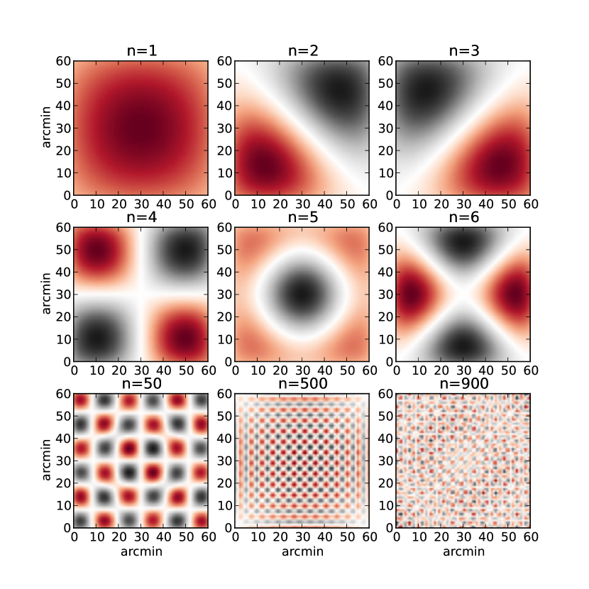
Figure 1.— A sample of nine of the 4096 KL eigenmodes of a $1^{\circ}\times 1^{\circ}$ patch of the sky partitioned into $64\times 64$ pixels. Black is positive, red is negative, and each mode has unit norm. The modes are calculated from the theoretical shear correlation function (see Section 2.3). As a consequence of the isotropy of the cosmic shear field, the covariance matrix – and thus the associated eigenmodes – are purely real (see Section 3.1).

3. Testing KL Reconstructions

In this section we show results of the KL analysis of shear fields for a sample geometry. In Section 3.1 we discuss the general properties of shear KL modes for unmasked fields, while in Section 3.2 we discuss KL shear reconstruction in the presence of masking.

3.1. KL Decomposition of a Single Field

To demonstrate the KL decomposition of a shear field, we assume a square field of size $1^{\circ}\times 1^{\circ}$, divided into $64\times 64$ pixels. We assume a source galaxy density of $20\ \mathrm{arcmin}^{-2}$ – appropriate for a ground-based survey such as DES – and calculate the KL basis following the method outlined in Section 2.1. For the computation of the nonlinear matter power spectrum, we assume a flat $\Lambda$CDM cosmology with $\Omega_{M}=0.27$ at the present day, with the power spectrum normalization given by $\sigma_{8}=0.81$.

Figure 1 shows a selection of nine of the 4096 shear eigenmodes within this framework. The KL modes are reminiscent of 2D Fourier modes, with higher-order modes probing progressively smaller length scales. This characteristic length scale of the eigenmodes can be seen quantitatively in Figure 2. Here we have computed the rotationally averaged power spectrum $C_{\ell}$ for each individual Fourier mode, and plotted the power vertically as a density plot for each mode number. Because the KL modes are not precisely equivalent to the 2D Fourier modes, each contains power at a range of values in $\ell$. But the overall trend is clear: larger modes probe smaller length scales, and the modes are very close to Fourier in nature.

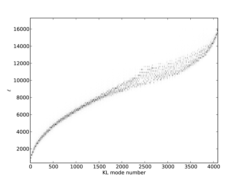
Figure 2.— The normalized power spectrum of each KL mode. For constant mode number, the figure represents a histogram of the power in that KL mode, normalized to a constant total power. KL modes represent a linear combination of Fourier modes, so that the power in each KL mode is spread over a range of $\ell$ values. Nevertheless, the general trend is clear: larger mode numbers are associated with larger wave numbers, and thus smaller length scales.

As noted in Section 2, one useful quality of a KL decomposition is its diagonalization of the signal and noise of the problem. To explore this property, we plot in the upper panel of Figure 3 the eigenvalue profile of these KL modes. By construction, higher-order modes have smaller KL eigenvalues. What is more, because the noise in the covariance matrix is whitened (see Section 2.2), the expectation of the noise covariance within each mode is equal to 1. Subtracting this noise from each eigenvalue gives the expectation value of the signal-to-noise ratio: thus we see that the expected signal-to-noise ratio of the eigenmodes is above unity only for the first 17 of the 4096 modes.

At first glance, this may seem to imply that only the first 17 or so modes are useful in a reconstruction. On the contrary: as seen in the lower panel of Figure 3, these first 17 modes contain only a small fraction of the total information in the shear field (This is not an unexpected result: cosmic shear measurements have notoriously low signal-to-noise ratios!) About 900 modes are needed to preserve an average of 70% of the total signal, and at this level, each additional mode has a signal-to-noise ratio of below $1/10$. The noisy input shear field can be exactly recovered by using all 4096 modes: in this case, though, the final few modes contribute two orders-of-magnitude more noise than signal.

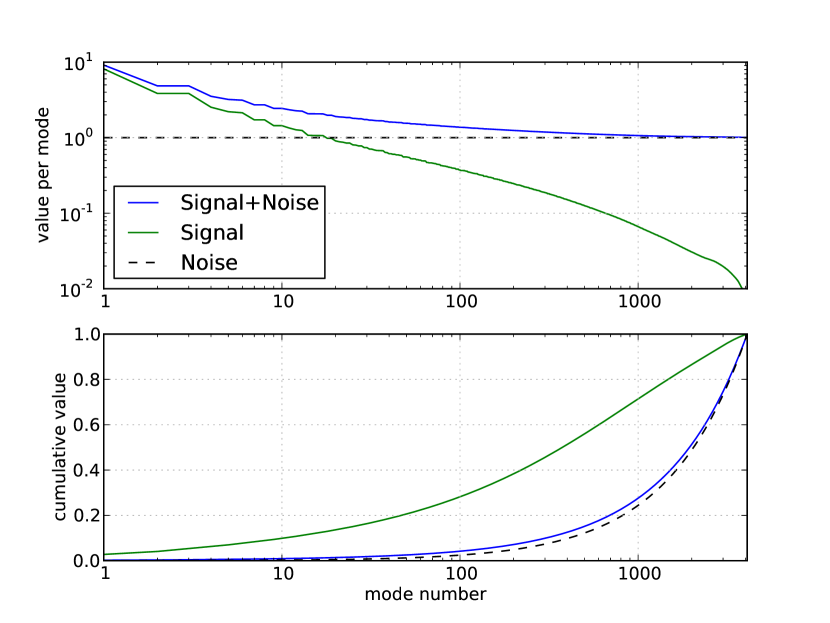
Figure 3.— The eigenvalues associated with the eigenmodes discussed in Figure 1. By construction, the eigenvalue is proportional to the sum of signal and noise within each mode. The upper figure shows the value per mode, while the lower figure shows the normalized cumulative value. The stepped-pattern evident in the upper panel is due to the presence of degenerate eigenmodes which have identical eigenvalues (e.g. modes $n=2$ and $n=3$, related by parity as evident in Figure 1). Because the eigenmodes are computed from a whitened covariance matrix (see Section 2.2), the noise contribution within each mode is equal to 1. Subtracting this contribution leads to the plot of signal only: this shows that the signal-to-noise ratio is above unity only for the first $17$ modes. Still, as seen in the lower panel, higher modes are required: the first $17$ modes account for only $12\%$ of the signal on average. To recover $70\%$ of the signal in a particular reconstruction requires about 1000 modes. At this point, each additional mode has a signal-to-noise ratio of less than $0.1$. Such a small signal-to-noise ratio is a well-known aspect of cosmic shear studies.

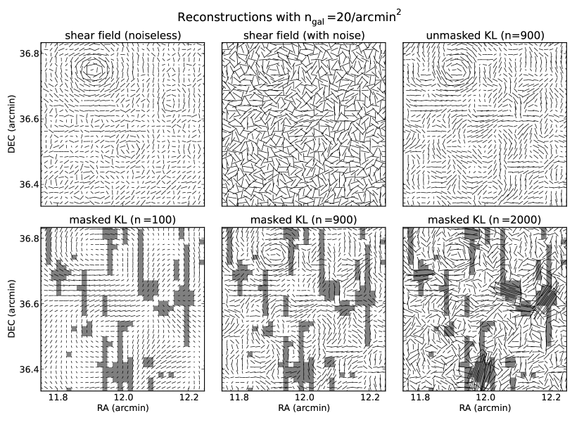
Figure 4.— This figure illustrates the reconstruction of a small patch of masked shear from simulated shear catalog. upper panels: The underlying noiseless shear signal (left), the observed, noisy shear signal (middle), and the unmasked reconstruction with 900 modes and $\alpha=0.15$. The amplitude of the noise is calculated using an intrinsic ellipticity $\sigma_{\epsilon}=0.3$, with an average number density of $n_{gal}=20\ \mathrm{arcmin}^{-2}$. The large peak in the upper portion of the figure is well-recovered by the KL reconstruction. lower panels: The KL reconstruction of the shear in the presence of 20% masking, with increasing number of modes $n$. The mask is represented by the shaded regions in panels: within these regions, the value of the shear is recovered through KL interpolation (see Section 2.5). We see in this progression the effect of the KL cutoff choice: using too few modes leads to loss of information, while using too many modes leads to over-fitting within the masked regions (See Appendix A for a discussion of the choice of number of modes).

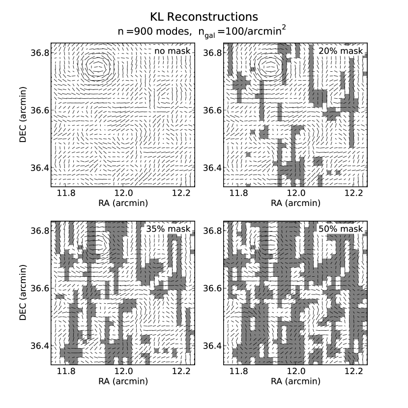
Figure 5.— Here we show the same field as in Figure 4, reconstructed using $n=900$ modes, with increasing levels of mask coverage. The density of source galaxies has been increased to 100 arcmin^-2, typical of a space-based weak lensing survey. At this noise level, smaller halos can be detected within the unmasked KL reconstruction (upper-left panel). Even at a 50% masking level, the large peak at (RA,DEC) = (11.9,36.75) is adequately recovered.

3.2. Testing KL Interpolation

To test this KL interpolation technique, we use simulated shear catalogs. These catalogs contain 220 square degrees of simulated shear maps, computed using a ray-tracing grid through a cosmological N-body simulation of the standard $\Lambda$-CDM model. The shear signal is computed at the locations of background galaxies with a median redshift of about 0.7. Galaxies are incorporated in the simulation using the ADDGALS algorithm (Wechsler, 2004, Wechsler et al. in preperation), tuned to the expected observational characteristics of the DES mission.

We pixelize this shear field using the same pixel size as above: $64\times 64$ pixels per square degree. To perform the KL procedure on the full field with this angular resolution would lead to a data vector containing over $10^{6}$ elements, and an associated covariance matrix containing $10^{12}$ entries. A full eigenvalue decomposition of such a matrix is computationally infeasible, so we reconstruct the field in $1^{\circ}\times 1^{\circ}$ tiles, each $64\times 64$ pixels in size. To reduce edge effects between these tiles, we use only the central $0.5^{\circ}\times 0.5^{\circ}$ region of each, so that covering the 300 square degree field requires 1200 tiles.

In order to generate a realistic mask over the field area, we follow the procedure outlined in Hikage et al. (2010) which generates pixel-level masks characteristic of point-sources, saturation spikes, and bad CCD regions. We tune the mask so that 20% of the shear pixels have no data. The geometry of the mask over a representative patch of the field can be seen in the lower panels of Figure 4, where we also show the result of the KL interpolation using 900 out of 4096 modes, with $\alpha=0.15$ (For a discussion of these parameter choices, see Appendix A).

The upper panels of Figure 4 give a qualitative view of the difficulty of cosmic shear measurements. The top left panel shows the noiseless shear across the field, while the top right panel shows the shear with shape noise for a DES-type survey ($\sigma_{\epsilon}=0.3$, $\bar{n}_{gal}=20\ \mathrm{arcmin}^{-2}$). To the eye, the signal seems entirely washed out by the noise. Nevertheless, the shear signal is there, and can be fairly well-recovered using the first 900 KL modes (middle-left panel). For masked data, we must resort to the techniques of Section 2.5 to fill-in the missing data. The middle-right panel shows this reconstruction, with gray shaded regions representing the masked area. A visual comparison of the masked and unmasked $n=900$ panels of Figure 4 confirms qualitatively that the KL interpolation is performing as desired. This is especially apparent near the large cluster located at (RA,DEC)=(11.9,36.7). The remaining two lower panels of Figure 4 show cases of over-fitting and under-fitting of the shear data. If too few KL modes are used, the structure of the input shear field is lost. If too many KL modes are used, the masked regions are over-fit, causing the interpolated shear values to become unnaturally large. This observation suggests one rubric by which the ideal number of modes can be chosen; see the discussion in Appendix A.

It is interesting to explore the limits of this interpolation algorithm. Figure 5 shows the KL reconstruction with increasing masked fractions, using a noise level typical of space-based lensing surveys $(n_{gal}=100{\rm arcmin}^{-2})$ Though the quality of the reconstruction understandably degrades, the lower panels show that large features can be recovered even with up to 50% of the pixels masked.

For a quantitative analysis of the effectiveness of the KL interpolation in convergence mapping, and the potential biases it introduces, a large-scale statistical measure is most appropriate. In the following sections, we test the utility of this KL interpolation scheme within the framework of shear peak statistics.

4. Shear Peak Statistics

It has long been recognized that much useful cosmological information can be deduced from the masses and spatial distribution of galaxy clusters (e.g. Press & Schechter, 1974). Galaxy clusters are the largest gravitationally bound objects in the universe, and as such are exponentially sensitive to cosmological parameters (White et al., 1993). The spatial distribution of clusters and redshift evolution of their abundance and clustering is sensitive to both geometrical effects of cosmology, as well as growth of structure. Because of this, cluster catalogs can be used to derive constraints on many interesting cosmological quantities, including the matter density $\Omega_{M}$ and power spectrum normalization $\sigma_{8}$ (Lin et al., 2003), the density and possible evolution of dark energy (Linder & Jenkins, 2003; Vikhlinin et al., 2009), primordial non-gaussianities (Matarrese et al., 2000; Grossi et al., 2007), and the baryon mass fraction (Lin et al., 2003; Giodini et al., 2009).

Various methods have been developed to measure the mass and spatial distribution of galaxy clusters, and each are subject to their own difficult astrophysical and observational biases. They fall into four broad categories: optical or infrared richness, X-ray luminosity and surface brightness, Sunyaev-Zeldovich decrement, and weak lensing shear.

While it was long thought that weak gravitational lensing studies would lead to robust, purely mass-selected cluster surveys, it has since become clear that shape noise and projection effects limit the usefulness of weak lensing in determining the 3D cluster mass function (Hamana et al., 2004; Hennawi & Spergel, 2005; Mandelbaum et al., 2010; VanderPlas et al., 2011). The shear observed in weak lensing is non-locally related to the convergence, a measure of projected mass along the line of sight. The difficulty in deconvolving the correlated and uncorrelated projections in this quantity leads to difficulties in relating these projected peak heights to the masses of the underlying clusters in three dimensions. Recent work has shown, however, that this difficulty in relating the observed quantity to theory may be overcome through the use of statistics of the projected density itself.

Marian et al. (2009, 2010) first explored the extent to which 2D projections of the 3D mass field trace cosmology. They found, rather surprisingly, that the statistics of the projected peaks closely trace the statistics of the 3D peak distribution: in N-body simulations, both scale with the Sheth & Tormen (1999) analytic scaling relations. The same correlated projections which bias cluster mass estimates contribute to a usable signal: statistics of projected mass alone can provide useful cosmological constraints, without the need for bias-prone conversions from peak height to cluster mass.

A host of other work has explored diverse aspects of these shear peak statistics, including tests of these methods with ensembles of N-body simulations (Wang et al., 2009; Kratochvil et al., 2010; Dietrich & Hartlap, 2010), the performance of various filtering functions and peak detection statistics (Pires et al., 2009; Schmidt & Rozo, 2010; Kratochvil et al., 2011), exploration of the spatial correlation of noise with signal within convergence maps (Fan et al., 2010), and exploration of shear-peak constraints on primordial non-gaussianity (Maturi et al., 2011). The literature has yet to converge on the ideal mapping procedure: convergence maps, gaussian filters, various matched filters, wavelet transforms, and more novel filters are explored within the above references. There is also variation in how a “peak” is defined: simple local maxima, “up-crossing” criteria, fractional areas above a certain threshold, connected-component labeling, hierarchical methods, and Minkowski functionals are all shown to be useful. Despite diverse methodologies, all the above work confirms that there is useful cosmological information within the projected peak distribution of cosmic shear fields, and that this information adds to that obtained from 2-point statistics alone.

4.1. Aperture Mass Peaks

Based on this consensus, we use shear peak statistics to explore the possible bias induced by the KL interpolation method outlined above. We follow the aperture mass methodology of Dietrich & Hartlap (2010): The aperture mass magnitude at a point $\vec{\theta}_{0}$ is given by

$$M_{\rm ap}(\vec{\theta_{0}})=\int_{\Omega}d^{2}\theta Q_{\rm NFW}(\vartheta=|\vec{\theta}-\vec{\theta}_{0}|)\gamma_{t}(\vec{\theta};\vec{\theta}_{0})$$ (18)

where $\gamma_{t}(\vec{\theta};\vec{\theta}_{0})$ is the component of the shear at location $\vec{\theta}$ tangential to the line $\vec{\theta}-\vec{\theta}_{0}$, and $Q_{\rm NFW}$ is the NFW-matched filter function defined in Schirmer et al. (2007):

$$Q_{\rm NFW}(x;x_{c})\propto\frac{1}{1+e^{6-150x}+e^{-47+50x}}\frac{\tanh(x/x_{c})}{x/x_{c}}$$ (19)

with $x=\vartheta/\vartheta_{\rm max}$ and $x_{c}$ a free parameter. We follow Dietrich & Hartlap (2010) and set $\vartheta_{\rm max}=5.6\ \mathrm{arcmin}$ and $x_{c}=0.15$. The integral in Equation 18 is over the whole sky, though the filter function $Q$ effectively cuts this off at a radius $\vartheta_{\rm max}$. In the case of our pixelized shear field, the integral is converted to a discrete sum over all pixels, with $\vartheta$ equal to the distance between the pixel centers:

$$M_{\rm ap}(\vec{\theta}_{i})=\sum_{j}Q_{\rm NFW}(\vartheta_{ij})\gamma_{t}(\vec{\theta}_{i};\vec{\theta}_{j})$$ (20)

where we have defined $\vartheta_{ij}\equiv|\vec{\theta}_{i}-\vec{\theta}_{j}|$.

We can similarly compute the B-mode aperture mass, by substituting $\gamma_{t}\to\gamma_{\times}$ in Equations 18-20 (Crittenden et al., 2002). For pure gravitational weak lensing with an unbiased shear estimator, the B-mode signal is expected to be negligible, though second-order effects such as source clustering and intrinsic alignments can cause contamination on small angular scales (Crittenden et al., 2002; Schneider et al., 2002b) These effects aside, the B-mode signal can be used as a rough estimate of the systematic bias of a particular analysis method.

For our study, the aperture mass is calculated with the same resolution as the shear pixelization: $64^{2}$ pixels per square degree. A pixel is defined to be a peak if its value is larger than that of the surrounding eight pixels: a simple local maximum criterion.

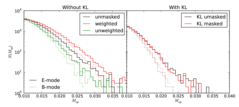
Figure 6.— Comparison of the masked and unmasked peak distributions. left panel: the peak distributions without the use of KL. The black line is the result with no masking, while the red and green lines show the two naïve methods of correcting for the mask (see Section 4.2). right panel: the masked and unmasked peak distributions after applying KL. Neither naïve method of mask-correction adequately recovers the underlying peak distribution. It is evident, however, that the KL-based interpolation procedure recovers a mass map with a similar peak distribution to the unmasked KL map. It should be noted that the unmasked peak distribution (black line, left panel) is not identical to the unmasked peak distribution after application of KL (black line, right panel). This difference is addressed in Figure 7.

4.2. The Effects of Masking

When a shear peak statistic is computed across a field with masked regions, the masking leads to a bias in the peak height distribution (see Section 5 below). Moreover, due to the non-local form of the aperture mass statistic, a very large region is affected: in our case, a single masked pixel biases the aperture mass measurement of an area of size $\pi(2\vartheta_{\rm max})^{2}\approx 400\ {\rm arcmin}^{2}$. There are two naïve approaches one could use when measuring the aperture mass in this situation:

Unweighted:

Here we simply set the shear value within each masked pixel to zero, and apply Equation 20. The shear within the masked regions do not contribute to the peaks, so the height of the peaks will be underestimated.

Weighted:

Here we implement a weighting scheme which re-normalizes the filter $Q_{\rm NFW}$ to reflect the reduced contribution from masked pixels. The integral in equation 18 is replaced by the normalized sum:

$$M_{\rm ap}(\vec{\theta}_{i})=\frac{\sum_{j}Q_{\rm NFW}(\vartheta_{ij})\gamma_{t}(\vec{\theta}_{j})w(\vec{\theta}_{j})}{\sum_{j}Q_{\rm NFW}(\vartheta_{ij})w(\vec{\theta}_{j})}$$ (21)

where $w(\vec{\theta}_{j})=0$ if the pixel is masked, and $1$ otherwise. This should correct for the underestimation of peak heights seen in the unweighted case.

In order to facilitate comparison between this weighted definition of $M_{\rm ap}$ and the normal definition used in the unmasked and unweighted cases, we normalize the latter by $\sum_{j}Q_{\rm NFW}(\vec{\theta}_{ij})$, which is a constant normalization across the field.

Note that in both cases, it is the shear that is masked, not the $M_{\rm ap}$ peaks. Aperture mass is a non-local measure, so that the value can be recovered even within the masked region. This means that masking will have a greater effect on the observed magnitude of the peaks than it will have on the count. In particular, on the small end of the peak distribution, where the peaks are dominated by shape noise, the masking of the shear signal is likely to have little effect on the distribution of peak counts. This can be seen in Figure 7.

4.3. $M_{\rm ap}$ Signal-to-Noise

It is common in shear peak studies to study signal-to-noise peaks rather than directly study aperture-mass or convergence peaks (e.g.  Wang et al., 2009; Dietrich & Hartlap, 2010; Schmidt & Rozo, 2010). We follow this precedent here. The aperture mass (Eqn. 20) is defined in terms of the tangential shear. Because we assume that the shear measurement is dominated by isotropic, uncorrelated shape noise, the noise covariance of $M_{\rm ap}$ can be expressed

$$[\boldsymbol{\mathcal{N}}_{M}]_{ij} \equiv \langle M_{\rm ap}(\vec{\theta}_{i})M_{\rm ap}(\vec{\theta}_{j})\rangle$$ (22)

$$= \frac{1}{2}\sum_{k}Q^{2}_{\rm NFW}(\vartheta_{ik})[\boldsymbol{\mathcal{N}}_{\gamma}]_{kk}\delta_{ij}$$

where we have used the fact that shape noise is uncorrelated: $[\boldsymbol{\mathcal{N}}_{\gamma}]_{ij}=\langle n_{i}n_{j}\rangle\propto\delta_{ij}$.

In the case of a KL-reconstruction of a masked shear field, the reconstructed shear has non-negligible correlation of noise between pixels. From Equations 15-17, it can be shown that

$$\boldsymbol{\mathcal{N}}_{\hat{\gamma}} \equiv \langle\boldsymbol{\hat{\gamma}}\boldsymbol{\hat{\gamma}}^{\dagger}\rangle$$ (23)

$$= \boldsymbol{\mathcal{N}}_{\gamma}^{1/2}\boldsymbol{\Psi}\boldsymbol{M}^{-1}\boldsymbol{\Psi}^{\dagger}\boldsymbol{W}^{2}\boldsymbol{\Psi}\boldsymbol{M}^{-1}\boldsymbol{\Psi}^{\dagger}\boldsymbol{\mathcal{N}}_{\gamma}^{1/2}$$

The covariance matrix $\boldsymbol{\mathcal{N}}_{\hat{\gamma}}$ is no longer diagonal, but the noise remains isotropic under the linear transformation, so that $\boldsymbol{\mathcal{N}}_{\hat{\gamma}_{t}}=\boldsymbol{\mathcal{N}}_{\hat{\gamma}}/2$. The aperture mass noise covariance can thus be calculated in a similar way to the non-KL case:

$$[\boldsymbol{\mathcal{N}}_{M}]_{ij}=\frac{1}{2}\sum_{k}\sum_{\ell}Q_{\rm NFW}(\vartheta_{ik})Q_{\rm NFW}(\vartheta_{j\ell})[\boldsymbol{\mathcal{N}}_{\hat{\gamma}}]_{k\ell}.$$ (24)

This expression can be computed through standard linear algebraic techniques. The aperture mass signal-to-noise in each pixel is given by

$$[S/N]_{i}=M_{\rm ap}(\vec{\theta}_{i})/\sqrt{[\boldsymbol{\boldsymbol{\mathcal{N}}_{M}}]_{ii}}$$ (25)

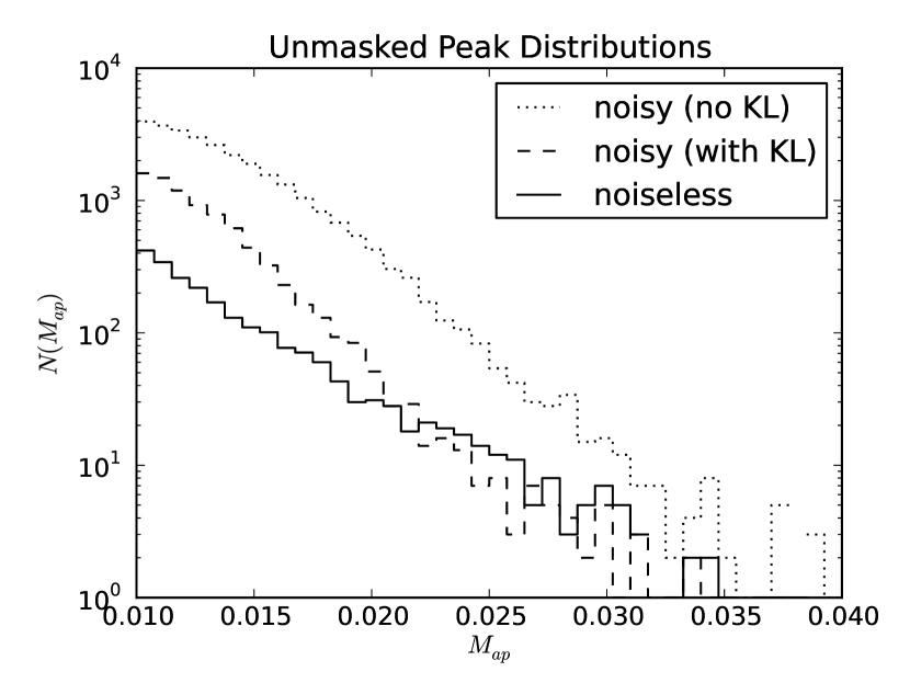
Figure 7.— Comparison of the distribution of $M_{\rm ap}$ peaks for unmasked shear, before and after filtering the field with KL (dotted line and dashed line, respectively). The peak distribution in the absence of noise is shown for comparison (solid line). It is clear that the addition of shape noise leads to many spurious $M_{\rm ap}$ peaks: noise peaks outnumber true peaks by nearly a factor of 10 for smaller peak heights. Filtering by KL reduces these spurious peaks by about a factor of 3, and for larger peaks leads to a distribution similar in scale to that of the noiseless peaks.

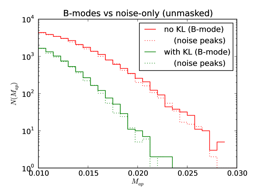
Figure 8.— The comparison between B-mode peak distributions and the peak distributions for a shear field composed entirely of noise. As expected, the B-mode peak distributions are largely consistent with being due to noise only. Because of this, we can use B-mode peaks as a rough proxy for the noise.

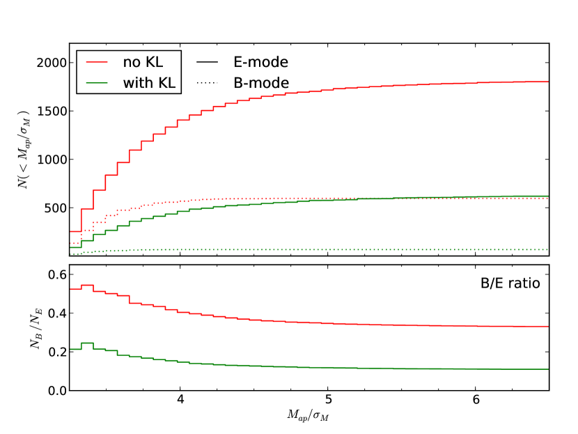
Figure 9.— top panel: The cumulative distributions of peaks in signal-to-noise, for peaks with $M_{\rm ap}/\sigma_{M}>3.25$. This is the statistic used by Dietrich & Hartlap (2010) to discriminate between cosmological models. bottom panel: The ratio of B-mode to E-mode peak distributions. Filtration by KL reduces the relative number of B-mode peaks by about 1/3. Because B-mode peaks are a proxy for contamination by shape noise (see Figure 8), this indicates that KL-filtration results in peak distributions less affected by statistical errors. KL also reduces the total number of both E and B peaks by about 2/3; this effect can also be seen in Figure 7.

5. Discussion

5.1. $M_{\rm ap}$ Peak Distributions

In Figures 6-9 we compare the peak distribution obtained with and without KL. We make three broad qualitative observations which point to the efficacy of KL in interpolation of masked shear fields, and in the filtration of shape-noise from these fields. We stress the qualitative nature of these results: quantifying these observations in a statistically rigorous way would require shear fields from an ensemble of cosmology simulations, which is beyond the scope of this work. These results nevertheless point to the efficacy of KL analysis in this context.

KL filtration corrects for the bias due to masking. Figure 6 compares the effect of masking on the resulting peak distributions with and without KL. The left panel shows the unmasked noisy peak distribution, and the masked peak distributions resulting from the weighted and unweighted approaches described in Section 4.2. Neither method of accounting for the masking accurately recovers the unmasked distribution of peak heights. The unweighted approach (green line) leads to an underestimation of peak heights. This is to be expected, because it does not correct for the missing information in the masked pixels. The weighted approach, on the other hand, over-estimates the counts of the peaks. We suspect this is due to an analog of Eddington bias: the lower signal-to-noise ratio of the weighted peak statistic leads to a larger scatter in peak heights. Because of the steep slope of the peak distribution, this scatter preferentially increases the counts of larger peaks. This suspicion is confirmed by artificially increasing the noise in the unmasked peak function. Increasing $\sigma_{\epsilon}$ from 0.30 to 0.35 in the unmasked case results in a nearly identical peak function to the weighted masked case.

The right panel of Figure 6 shows that when KL is applied to the shear field, the distribution of the masked and unmasked peaks is very close, both for E-mode and B-mode peaks. This indicates the success of the KL-based interpolation outlined in Section 2.5. Even with 20% of the pixels masked, the procedure can recover a nearly identical peak distribution as from unmasked shear.

KL filtration reduces the number of noise peaks. Comparison of the unmasked lines in the left and right panels of Figure 6 shows that application of KL to a shear field results in fewer peaks at all heights. This is to be expected: when a reconstruction is performed with fewer than the total number of KL modes, information of high spatial frequency is lost. In this way, KL acts as a sort of low-pass filter tuned to the particular signal-to-noise characteristics of the data. Figure 7 over-plots the KL and non-KL peak distributions with the noiseless peak distribution. From this figure we see that the inclusion of shape noise results in nearly an order-of-magnitude more peaks than the noiseless case. The effect of noise on peak counts lessens slightly for higher-$M_{\rm ap}$ peaks: this supports the decision of Dietrich & Hartlap (2010) to limit their distributions to peaks with a signal-to-noise ratio greater than 3.25: the vast majority of peaks are lower magnitude, and are overwhelmed by the effect of shape noise.

Omission of higher-order KL modes of shear field reduces the number of these spurious peaks by a factor of 3 or more. For low-magnitude peaks, $(M_{\rm ap}\lesssim 0.02)$, KL still produces peak counts which are dominated by noise. For higher-magnitude peaks, the number of observed KL peaks more closely approaches the number of peaks in the noiseless case.

KL filtration reduces the presence of B-modes. To first order, weak lensing shear is expected to consist primarily of curl-free, E-mode signal. Because of this, the presence of B-modes can indicate a systematic effect. It is not obvious that filtration by KL will maintain this property: as noted in Section 2.4, KL modes individually are agnostic to E-mode and B-mode information. E&B information is only recovered within a complex-valued linear combination of the set KL modes.

Figure 8 shows a comparison between the unmasked B-mode peak functions from Figure 6 and the associated E-mode peak functions due to shape-noise only. For both the non-KL version and the KL version, the B-mode peak distributions closely follow the distributions of noise peaks. This supports the use of B-mode peaks as a proxy for the peaks due to shape noise, even when truncating higher-order KL modes.

The near-equivalence of B-modes and noise-only peaks shown in Figure 8 suggests a way of recovering the true peak function, by subtracting the B-mode count from the E-mode count as a proxy for the shape noise. This approach has one fatal flaw: because it involves computing the small difference between two large quantities, the result has extremely large uncertainties. It should be noted that this noise contamination of small peaks is not an impediment to using this method for cosmological analyses: the primary information in shear peak statistics is due to the high signal-to-noise peaks.

In the top panel of Figure 9, we show the cumulative distribution of peaks in signal-to-noise, for peaks with $S/N>3.25$: the quantity used as a cosmological discriminant in Dietrich & Hartlap (2010). The difference in the total number of E-mode peaks in the KL and non-KL approaches echoes the result seen in Figure 7: truncation of higher-order KL modes acts as a low-pass filter, reducing the total number of peaks by a factor of $\sim 3$. More interesting is the result shown in the lower panel of Figure 9, where the ratio of B-mode peak counts to E-mode peak counts is shown. Before application of KL, the B-mode contamination is above 30%. Filtration by KL reduces this contamination by a factor of $\sim 3$, to about 10%. This indicates that the truncation of higher-order KL modes leads to a preferential reduction of the B-mode signal, which traces the noise. This is a promising observation: the counts of high signal-to-noise peaks, which offer the most sensitivity to cosmological parameters (Dietrich & Hartlap, 2010), are significantly less contaminated by noise after filtering and reconstruction with KL. This is a strong indication that the use of KL could improve the cosmological constraints derived from studies of shear peak statistics.

Note that in Figure 9 we omit the masked results for clarity. The masked cumulative signal-to-noise peak functions have B/E ratios comparable to the unmasked versions, so the conclusions here hold in both the masked and unmasked cases.

5.2. Remaining Questions

The above discussion suggests that KL analysis of masked shear fields holds promise in constraining cosmological parameters of shear peaks in both masked and unmasked fields. KL greatly reduces the number of spurious noise peaks at all signal-to-noise levels. It minimizes the bias between masked and unmasked constructions, and leads to a factor of 3 suppression of the B-mode signal, which is a proxy for the spurious signal introduced through shape noise.

The question remains, however, how much cosmological information is contained in the KL peak functions. The reduction in level of noise peaks is promising, but the omission of higher-order modes in the KL reconstruction leads to a smoothing of the shear field on scales smaller than the cutoff mode. This smoothing could lead to the loss of cosmologically useful information. In this way, the choice of KL mode cutoff can be thought of as a balance between statistical and systematic error. The effect of these competing properties on cosmological parameter determination is difficult to estimate. Quantifying this effect will require analysis within a suite of synthetic shear maps, similar to the approach taken in previous studies (e.g. Dietrich & Hartlap, 2010; Kratochvil et al., 2010), and will be the subject of future work.

Another possible application of KL in weak lensing is to use KL to directly constrain 2-point information in the measured shear data. In contrast to the method outlined in the current work, KL basis functions can be computed for the unmasked region only. The projection of observed data onto this basis can be used to directly compute cosmological parameters via the 2-point function, without ever explicitly calculating the power spectrum. This is similar to the approach taken for galaxy counts in Vogeley & Szalay (1996). We explore this approach in a followup work.

Acknowledgments: We are very grateful to Risa Wechsler, Michael Busha, and Matt Becker for providing us simulated shear catalogs. The simulation used to produce the catalogs is one of the Carmen simulations, a 1 Gpc simulation run by M. Busha as part of the LasDamas project. We thank Alex Szalay for helpful discussions regarding KL analysis in cosmological contexts. Support for this research was provided by DOE Grant DESC0002607. This research was partially supported by NSF AST-0709394 and NASA NNX07-AH07G.

Appendix A Choice of KL Parameters

The KL analysis outlined in Section 2 has only two free parameters: the number of modes $n$ and the Wiener filtering level $\alpha$. Each of these parameters involves a trade-off: using more modes increases the amount of information used in the reconstruction, but at the expense of a decreased signal-to-noise ratio. Decreasing the value of $\alpha$ to $0$ reduces the smoothing effect of the prior, but can lead to a nearly singular convolution matrix $\boldsymbol{M}_{(n,\alpha)}$, which results in unrealistically large shear values in the poorly-constrained areas areas of the map (i.e. masked regions).

To inform our choice of the number of modes $n$, we recall the trend of spatial scale with mode number seen in Figure 2. Our purpose in using KL is to allow interpolation in masked regions. To this end, the angular scale of the mask should inform the choice of angular scale of the largest mode used. An eigenmode which probes scales much smaller than the size of a masked region will not contribute meaningful information to the reconstruction within that masked region. Considering the pixels within our mask, we find that 99.5% of masked pixels are within 2 pixels of a shear measurement. This corresponds to an angular scale of $\ell=6140$. Consulting Figure 2, we see that modes larger than about $n=900$ out of 4096 will probe length scales significantly smaller than the mask scale. Thus, we choose $n=900$ as an appropriate cutoff for our reconstructions.

To inform our choice of the Wiener filtering level $\alpha$, we examine the agreement between histograms of $M_{\rm ap}$ peaks for a noise-only DES field with and without masking (see Section 4). We find that for large (small) values of $\alpha$, the number of high-$M_{\rm ap}$ peaks is underestimated (overestimated) in the masked case as compared to the unmasked case. Empirically, we find that the two agree at $\alpha=0.15$; we choose this value for our analysis. Note that this tuning is done on noise-only reconstructions, which can be generated for observed data by assuming that shape noise dominates:

$$[\boldsymbol{\mathcal{N}}_{\gamma}]_{ij}=\frac{\sigma_{\epsilon}}{n_{i}^{2}}\delta_{ij}.$$ (A1)

The $\alpha$-tuning can thus be performed on artificial noise realizations which match the observed survey characteristics.

We make no claim that $(n,\alpha)=(900,0.15)$ is the optimal choice of free parameters for KL: determining this would involve a more in-depth analysis. They are simply well-motivated choices which we use to make a case for further study.

References

- Bartelmann & Schneider (2001) Bartelmann, M., & Schneider, P. 2001, Phys. Rep., 340, 291
- Connolly & Szalay (1999) Connolly, A. J., & Szalay, A. S. 1999, AJ, 117, 2052
- Connolly et al. (1995) Connolly, A. J., Szalay, A. S., Bershady, M. A., Kinney, A. L., & Calzetti, D. 1995, AJ, 110, 1071
- Crittenden et al. (2002) Crittenden, R. G., Natarajan, P., Pen, U., & Theuns, T. 2002, ApJ, 568, 20
- Dietrich & Hartlap (2010) Dietrich, J. P., & Hartlap, J. 2010, MNRAS, 402, 1049
- Fan et al. (2010) Fan, Z., Shan, H., & Liu, J. 2010, ApJ, 719, 1408
- Giodini et al. (2009) Giodini, S. et al. 2009, ApJ, 703, 982
- Grossi et al. (2007) Grossi, M., Dolag, K., Branchini, E., Matarrese, S., & Moscardini, L. 2007, MNRAS, 382, 1261
- Hamana et al. (2004) Hamana, T., Takada, M., & Yoshida, N. 2004, MNRAS, 350, 893
- Hennawi & Spergel (2005) Hennawi, J. F., & Spergel, D. N. 2005, ApJ, 624, 59
- Hikage et al. (2010) Hikage, C., Takada, M., Hamana, T., & Spergel, D. 2010, ArXiv e-prints
- Kaiser et al. (1995) Kaiser, N., Squires, G., & Broadhurst, T. 1995, ApJ, 449, 460
- Kilbinger & Munshi (2006) Kilbinger, M., & Munshi, D. 2006, MNRAS, 366, 983
- Kratochvil et al. (2010) Kratochvil, J. M., Haiman, Z., & May, M. 2010, Phys. Rev. D, 81, 043519
- Kratochvil et al. (2011) Kratochvil, J. M., Lim, E. A., Wang, S., Haiman, Z., May, M., & Huffenberger, K. 2011, in Bulletin of the American Astronomical Society, Vol. 43, American Astronomical Society Meeting Abstracts #217, #225.02–+
- Lin et al. (2003) Lin, Y., Mohr, J. J., & Stanford, S. A. 2003, ApJ, 591, 749
- Linder & Jenkins (2003) Linder, E. V., & Jenkins, A. 2003, MNRAS, 346, 573
- Mandelbaum et al. (2010) Mandelbaum, R., Seljak, U., Baldauf, T., & Smith, R. E. 2010, MNRAS, 405, 2078
- Marian et al. (2009) Marian, L., Smith, R. E., & Bernstein, G. M. 2009, ApJ, 698, L33
- Marian et al. (2010) —. 2010, ApJ, 709, 286
- Matarrese et al. (2000) Matarrese, S., Verde, L., & Jimenez, R. 2000, ApJ, 541, 10
- Matsubara et al. (2000) Matsubara, T., Szalay, A. S., & Landy, S. D. 2000, ApJ, 535, L1
- Maturi et al. (2011) Maturi, M., Fedeli, C., & Moscardini, L. 2011, ArXiv e-prints
- Munshi & Kilbinger (2006) Munshi, D., & Kilbinger, M. 2006, A&A, 452, 63
- Neyrinck et al. (2009) Neyrinck, M. C., Szapudi, I., & Szalay, A. S. 2009, ApJ, 698, L90
- Neyrinck et al. (2010) —. 2010, ArXiv e-prints
- Padmanabhan et al. (2003) Padmanabhan, N., Seljak, U., & Pen, U. L. 2003, New Astronomy, 8, 581
- Pires et al. (2009) Pires, S., Starck, J., Amara, A., Teyssier, R., Réfrégier, A., & Fadili, J. 2009, MNRAS, 395, 1265
- Pope et al. (2004) Pope, A. C. et al. 2004, ApJ, 607, 655
- Press & Schechter (1974) Press, W. H., & Schechter, P. 1974, ApJ, 187, 425
- Scherrer et al. (2010) Scherrer, R. J., Berlind, A. A., Mao, Q., & McBride, C. K. 2010, ApJ, 708, L9
- Schirmer et al. (2007) Schirmer, M., Erben, T., Hetterscheidt, M., & Schneider, P. 2007, A&A, 462, 875
- Schmidt & Rozo (2010) Schmidt, F., & Rozo, E. 2010, ArXiv e-prints
- Schneider et al. (2010) Schneider, P., Eifler, T., & Krause, E. 2010, A&A, 520, A116+
- Schneider et al. (1998) Schneider, P., van Waerbeke, L., Jain, B., & Kruse, G. 1998, MNRAS, 296, 873
- Schneider et al. (2002a) Schneider, P., van Waerbeke, L., Kilbinger, M., & Mellier, Y. 2002a, A&A, 396, 1
- Schneider et al. (2002b) Schneider, P., van Waerbeke, L., & Mellier, Y. 2002b, A&A, 389, 729
- Seo et al. (2011) Seo, H., Sato, M., Dodelson, S., Jain, B., & Takada, M. 2011, ApJ, 729, L11+
- Sheth & Tormen (1999) Sheth, R. K., & Tormen, G. 1999, MNRAS, 308, 119
- Smith et al. (2003) Smith, R. E. et al. 2003, MNRAS, 341, 1311
- Takada & Jain (2004) Takada, M., & Jain, B. 2004, MNRAS, 348, 897
- Tegmark (1997) Tegmark, M. 1997, ApJ, 480, L87+
- VanderPlas et al. (2011) VanderPlas, J. T., Connolly, A. J., Jain, B., & Jarvis, M. 2011, ApJ, 727, 118
- Vikhlinin et al. (2009) Vikhlinin, A. et al. 2009, ApJ, 692, 1060
- Vogeley & Szalay (1996) Vogeley, M. S., & Szalay, A. S. 1996, ApJ, 465, 34
- Wang et al. (2009) Wang, S., Haiman, Z., & May, M. 2009, ApJ, 691, 547
- Wechsler (2004) Wechsler, R. H. 2004, Clusters of Galaxies: Probes of Cosmological Structure and Galaxy Evolution
- White et al. (1993) White, S. D. M., Efstathiou, G., & Frenk, C. S. 1993, MNRAS, 262, 1023
- Yip et al. (2004a) Yip, C. W. et al. 2004a, AJ, 128, 585
- Yip et al. (2004b) —. 2004b, AJ, 128, 2603