Evidence for Anomalous Dust-Correlated Emission at 8 GHz

Abstract

In 1969 Edward Conklin measured the anisotropy in celestial emission at 8 GHz with a resolution of 16.2^∘ and used the data to report a detection of the CMB dipole. Given the paucity of 8 GHz observations over large angular scales and the clear evidence for non-power law Galactic emission near 8 GHz, a new analysis of Conklin’s data is informative. In this paper we compare Conklin’s data to that from Haslam et al. (0.4 GHz), Reich and Reich (1.4 GHz), and WMAP (23-94 GHz). We show that the spectral index between Conklin’s data and the 23 GHz WMAP data is $\beta=-1.7\pm 0.1$, where we model the emission temperature as $T\propto\nu^{\beta}$. Free-free emission has $\beta\approx-2.15$, synchrotron emission has $\beta\approx-2.7$ to $-3$. Thermal dust emission ($\beta\approx 1.7$) is negligible at 8 GHz. We conclude that there must be another distinct non-power law component of diffuse foreground emission that emits near 10 GHz, consistent with other observations in this frequency range. By comparing to the full complement of data sets, we show that a model with an anomalous emission component, assumed to be spinning dust, is preferred over a model without spinning dust at 5$\sigma$ ($\Delta\chi^{2}=31$). However, the source of the new component cannot be determined uniquely.

1. Introduction

Many observations have shown that there is diffuse dust-correlated emission at frequencies below 40 GHz where the thermal emission by dust grains is usually expected to be negligible. The effect was first seen at large angular scales in the COBE DMR data by Kogut et al. (1996), who attributed the phenomenon to the simple co-location of thermal dust and free-free emission. These observations were confirmed by ground based measurements at finer angular scales (de Oliveira-Costa et al., 1997; Leitch et al., 1997). Soon thereafter, it was realized that the dust-correlated emission might in fact be due to microwave emission by spinning dust grains (Jones, 1997; Draine & Lazarian, 1998). In other words, where there is more thermally emitting dust radiating at frequencies $\nu>100$ GHz, there is also more spinning dust emitting near $\nu\sim 20$ GHz. Since then, the correlated diffuse emission has been seen at high and low Galactic latitudes (de Oliveira-Costa et al., 1998, 1999; Leitch et al., 2000; Mukherjee et al., 2001; Hamilton & Ganga, 2001; Mukherjee et al., 2002, 2003; Bennett et al., 2003; Banday et al., 2003; Lagache, 2003; de Oliveira-Costa et al., 2004; Finkbeiner, 2004; Davies et al., 2006; Fernández-Cerezo et al., 2006; Boughn & Pober, 2007; Hildebrandt et al., 2007; Dobler & Finkbeiner, 2008a, b; Dobler et al., 2009; Miville-Deschênes et al., 2008; Ysard et al., 2010; Kogut et al., 2011; Gold et al., 2011). At large angular scales, WMAP (Bennett et al., 2003) suggested that this correlation could also be explained by variable-index synchrotron emission co-located with dusty star-forming regions. However, alternative and subsequent analyses gave more support to the spinning dust hypothesis and attributed the source of the correlation to a population of small spinning grains (de Oliveira-Costa et al., 2002; Lagache, 2003; Ysard et al., 2010; Macellari et al., 2011).

Dust-correlated emission at microwave frequencies has also been observed in more compact regions (e.g., Finkbeiner et al. (2002, 2004); Watson et al. (2005); Casassus et al. (2004); Battistelli et al. (2006); Casassus et al. (2006); Iglesias-Groth (2006); Casassus et al. (2008); Dickinson et al. (2009); Scaife et al. (2009); Murphy et al. (2010); Tibbs et al. (2010); Scaife et al. (2010a, b); Dickinson et al. (2010); Planck Collaboration et al. (2011); Vidal et al. (2011); Castellanos et al. (2011); López-Caraballo et al. (2011)). Most recently, the Planck satellite has shown in detail the presence of a non power-law component. A new component of emission is clearly seen in the Perseus and $\rho$ Ophiuchus regions (Planck Collaboration et al., 2011). The component is well modeled as spinning dust, although the range of gas temperatures is large.

It has long been realized that large area maps in the 5-20 GHz range would be ideal for separating free-free from variable-index synchrotron emission, spinning dust, or any other emission process. For diffuse sources, COSMOSOMAS (Hildebrandt et al., 2007) observed the sky between 11 and 17 GHz and identified a dust-correlated component, as did TENERIFE (de Oliveira-Costa et al., 1999) observing at 10 and 15 GHz. The ARCADE 2 experiment (Kogut et al., 2011) observed at 3, 8, and 10 GHz and also found evidence in support of a new component. Here, we show that Conklin’s 1969 data (Conklin, 1969a, b) further improve constraints in this frequency range and at large angular scales.

Although spinning dust is currently the preferred single hypothesis for explaining the correlation, there are $\sim 10$ free parameters in the spinning dust model (e.g., Ali-Haïmoud et al. (2009)); and there could be multiple processes, including magnetized dust emission (Draine & Lazarian, 1999), at work.

The rest of the paper is outlined as follows. We describe the observations in §2, discuss an interpretation of the observations in §3, and conclude in §4.

2. Conklin’s observations

Conklin’s observations took place on White Mountain in 1968 and 1969, using a coherent receiver at 8 GHz with an effective full width at half maximum beam of $\theta_{1/2}=16.2^{\circ}$. The radiometer Dicke-switched at 37 Hz between two $\theta^{H}_{1/2}=14.5^{\circ}$ feeds pointed $\pm 30^{\circ}$ from the zenith along an E-W baseline. The data were averaged over 4 minutes, the entire apparatus was rotated 180^∘ over one minute, data were averaged again for 4 more minutes, and finally the apparatus was rotated back to its original position. During each such ten-minute cycle, the temperature difference between the two feeds was recorded; Conklin reported the differences as “east”-“west.” The 10-min differences were then averaged with a 30-min FWHM Gaussian function, effectively broadening the beam profile to $16.2^{\circ}$ along the scan direction. The data we use, shown in Figure 1 and reported in Table 1, come from the Nature publication and Conklin’s Ph.D. thesis. For this analysis, we use Conklin’s raw data after subtracting the contribution from the now well-established dipole. The per-point error bars are deduced from the “probable error” reported in his thesis. They may be treated as independent. They are larger than the purely statistical error by a factor of 1.6 .

The measurements were made at a single celestial circle at $\delta=32^{\circ}$ as indicated in Figure 2. The highest amplitude point at RA$=300^{\circ}$ comes from when the “E” beam crosses the Galactic plane at $b=0^{\circ}$ and $l=69.5^{\circ}$, and the “W” beam is out of the plane. The “E” beam again crosses the Galactic plane at $l=176.4^{\circ}$.

After subtracting up to a 10 mK Galactic contribution by extrapolating the 404 MHz Pauliny-Toth & Shakeshaft map (Pauliny-Toth & Shakeshaft, 1962) to 8 GHz, Conklin reported a preliminary measurement of the dipole with amplitude $1.6\pm 0.8$ mK in the direction $\alpha=13$h. After Conklin’s 1969 Ph.D. thesis, this became $2.3\pm 0.9$ mK in the direction $\alpha=11$h as reported at the IAU 44 symposium (Conklin, 1972). Though the error bars include an estimate for a $\pm 0.1$ uncertainty in the Galactic index (the statistical uncertainty was $\approx 0.02~{}$mK), there were lingering doubts about the extrapolation (Webster, 1974). Neglecting the correction for the Earth’s motion, the WMAP dipole ($3.358\pm 0.017~{}$mK in direction $\alpha=11.19$h at $\delta=-6\fdg 90$ for the full sky) has amplitude $2.83~{}$mK at $\delta=32^{\circ}$, in excellent agreement.

Figure 1.— Conklin’s observations of the anisotropy at 8 GHz. The data are plotted for each differential E-W observation at $\delta=32^{\circ}$, with the now well-established dipole subtracted. The dashed line is the WMAP dipole. The offset is not constrained by the measurement. The peak at RA $\sim 300^{\circ}$ corresponds to the “E” beam crossing the Galactic plane at $b=0^{\circ}$ and $l=69.5^{\circ}$.

Table 1Data at 8GHz from Conklin (1969a, b).

RA	Total	Dipole-
(deg)	anisotropy (mK)	removed (mK)
0	$24.4\pm 1.13$	4.38
15	$19.8\pm 1.13$	0.60
30	$16.5\pm 1.13$	-1.94
45	$15.1\pm 1.13$	-2.86
60	$16.6\pm 1.13$	-1.00
75	$18.8\pm 1.13$	1.46
90	$21.3\pm 1.13$	3.81
105	$23.4\pm 1.13$	5.65
120	$24.7\pm 1.27$	6.42
135	$23.1\pm 1.27$	4.20
150	$22.1\pm 1.27$	2.39
165	$21.7\pm 1.27$	1.13
180	$22.1\pm 1.27$	0.65
195	$22.7\pm 1.27$	0.50
210	$23.0\pm 1.27$	0.10
225	$22.2\pm 1.27$	-1.31
240	$19.4\pm 1.27$	-4.50
255	$12.4\pm 1.27$	-11.6
270	$5.67\pm 1.27$	-18.3
285	$14.5\pm 1.27$	-9.13
300	$20.4\pm 1.13$	-2.82
315	$23.8\pm 1.13$	1.30
330	$29.3\pm 1.13$	7.58
345	$34.2\pm 1.13$	13.3

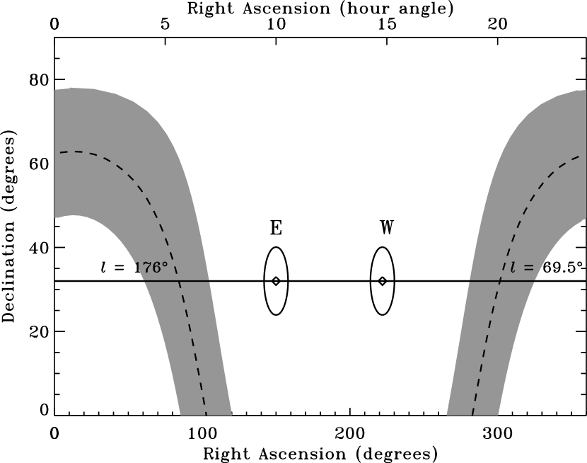
Figure 2.— Conklin’s observations with respect to the Galaxy. The “E” and “W” beams are separated by $60^{\circ}$ and are shown here as circles of diameter $16.2^{\circ}$. The dashed line marks the Galactic plane and the grey swath indicates $b=\pm 15^{\circ}$.

2.1. Calibration and beam characteristics

The system was calibrated with a 1K argon noise tube that injected power into the feeds through a cross guide coupler. This is effectively a full-beam calibrator. Conklin was mindful of the required stability and anchored all components with thermal straps every two inches. He measured the losses and reflections from all components and accounted for the atmosphere. A formal error is not reported but the system is similar to the one he used for a 10.7 GHz anisotropy measurement (Conklin & Bracewell, 1967) where he reported $\pm$10%, which we adopt.

Understanding the beam profile is critical for comparing to other data to assess the Galactic contribution. During observations, the sky drifts through the H-plane, the profile of which was measured. A measurement of the E-plane was not done. Based on his dimensions, we recomputed the full beam pattern using a more precise calculation (Sletten, 1988). We find an H-plane pattern $\theta^{H}_{1/2}=14.5^{\circ}$, in agreement with Conklin, and an E-plane pattern with $\theta^{E}_{1/2}=13.7^{\circ}$ as compared to Conklin’s $\theta^{E}_{1/2}=14^{\circ}$. For the full beam, we compute a 6% smaller solid angle. This translates into a possible bias that the peak-to-peak amplitude of the data is low by 6%. We account for this possibility in the analysis.

3. Comparison to other data sets

We compare Conklin’s data to that from Haslam (Haslam et al., 1981, 1982) at 0.408 GHz; Reich and Reich (Reich, 1982; Reich & Reich, 1986; Reich et al., 2001) at 1.42 GHz; WMAP at 23, 33, 44, 60, and 94 GHz (Jarosik et al., 2011); and the FDS map model 8 extrapolated to 94 GHz (Finkbeiner et al., 1999). We adopt calibration errors of 7%, 4%, and 2% for Haslam, Reich & Reich, and WMAP respectively. The statistical errors are negligible compared to the uncertainty on Conklin’s observations. We convolve the multi-frequency maps to the same 16.2^∘ resolution and extract differenced measurements at $\delta=32^{\circ}$ to compare to the Conklin data, shown in Figure 4. We do not account for the asymmetry in the Conklin effective beam, but test that varying the beam size by $2^{\circ}$ degrees has a negligible effect on conclusions. In all of our fits the calibration uncertainties dominate the statistical uncertainties.

We initially compare the emission, $I$, at $\nu_{0}=8$ GHz to the WMAP K-band emission ($\nu=23$ GHz), using a two parameter model,

$$I(\nu_{0},\hat{n})=I(\nu,\hat{n})(\nu_{0}/\nu)^{\beta}+A.$$ (1)

We fit for the index, $\beta$, and offset, $A$, finding a marginalized limit of $\beta=-1.7\pm 0.1$, with best-fit $\chi^{2}=64$ (reduced $\chi^{2}=1.34$). Because WMAP and Conklin are not observing the same mixture of foreground components, the high $\chi^{2}$ is not surprising. Figure 3 shows the marginalized distribution for the spectral index of the model. We include calibration error and the possible 6% calibration bias. The index is incompatible with free-free emission ($\beta=-2.15$), synchrotron emission $-3<\beta<-2.7$, or a “breaking” synchrotron index. Additionally, the WMAP best-fitting maximum entropy (MEM) model, excluding a spinning dust component, over-predicts the emission at 8 GHz by a factor of two. We conclude that there must exist another component of foreground emission.

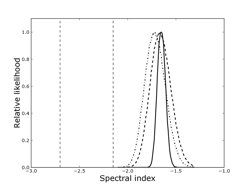
Figure 3.— Marginalized probability distribution for the effective spectral index between the Conklin 8 GHz data and the WMAP 23 GHz K-band data. The best fit model has $\chi^{2}=64.5$ for 46 degrees of freedom. The index is shallower than would be expected from sychrotron (left vertical dashed line) and free-free emission (right vertical dashed line), indicating the need for an additional component. The curves are, from left to right, Conklin plus a 6% systematic bias and calibration error, nominal Conklin with calibration error, and nominal Conklin without calibration error. The leftmost index shown is $\beta=-1.72\pm 0.1$.

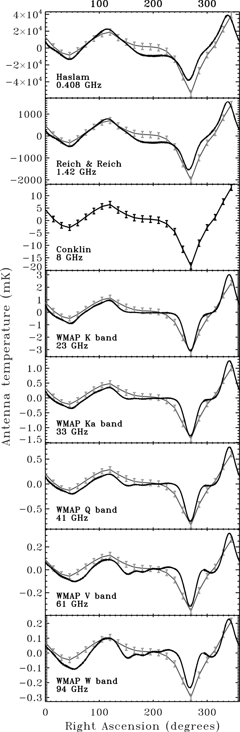
Figure 4.— Emission intensity at frequencies $0.4<\nu<94$ GHz in the $\delta=32^{\circ}$ strip surveyed by Conklin compared to the scaled $\nu_{0}=8$ GHz signal. The data from each map, $I(\nu)$, is fit to the Conklin data using $I(\nu)=s(\nu)I(\nu_{0})+A(\nu)$, and compared to the scaled Conklin data using the best-fitting $s(\nu)$ and $A(\nu)$. With multiple emission components, a global scaling of the 8 GHz data does not fully describe the foreground intensity.

To determine the scaling between Conklin’s data and each of the data sets in the range $\nu$=$0.4-94$ GHz, we fit $I(\nu)=s(\nu)I(\nu_{0})+A(\nu)$. Figure 4 shows how the intensity measured at each frequency, $I(\nu)$, compared to the scaled Conklin data, $s(\nu)I(\nu_{0})+A(\nu)$. The estimated scaling factors are reported in Table 2, with the goodness of fit. The closest fit is obtained between 8 GHz and the WMAP K band because these are the closest in the logarithm of the observation frequency. A simple power law extrapolation is a poor fit for more widely spaced frequencies as multiple components contribute to the emission. Figure 5 shows the frequency dependence of the estimated scaling factors $s(\nu)$ after multiplying by the rms of Conklin’s data. Consistent results are found by fitting to the $l=176^{\circ}$ or $l=69.5^{\circ}$ Galaxy crossings, the rms of each data set, or to the peak-to-peak amplitude as a function of frequency. The fit is dominated by the Galactic crossing regions.

Table 2Scaling factor between Conklin’s data and other data sets.

Data	Freq (GHz)	$s(\nu)$	$\chi^{2}$/DOF
Haslam	0.408	$2890\pm 130$	2.04
Reich	1.42	$107\pm 4.54$	1.75
Conklin	8	1	—
WMAP	23	$0.179\pm 0.0075$	1.33
WMAP	33	$0.0732\pm 0.0031$	1.54
WMAP	41	$0.0431\pm 0.0018$	1.81
WMAP	61	$0.0194\pm 0.00086$	2.69
WMAP	94	$0.0158\pm$0.00072	3.19

To find a physical model that fits Conklin’s observations as well as the Haslam, Reich and Reich, and WMAP data we perform a simultaneous fit to $s(\nu)$ in the range $0.4-94$ GHz. The model includes free-free, synchrotron, thermal dust, and spinning dust. We test the improvement in $\chi^{2}$ as we add a spinning dust component, using the model of Ali-Haïmoud et al. (2009). As free parameters, we take the total hydrogen number density $n_{\mathrm{H}}$ and the gas temperature $T$, assuming a single density and temperature can be used to model the global emission. For the other parameters, we use the values given by Ali-Haïmoud et al. (2009) in their sample spectrum and nominal parameters in Weingartner & Draine (2001) Table 1, line 7. Best fits are obtained with $n_{\mathrm{H}}$ = 20 cm^-3 and $T=300$K. The values of these parameters, however, would be affected by more refined models of the emission process (Draine, 2011). For the thermal dust emission, we consider two models: one in which the thermal dust amplitude is constrained by the FDS99 model, and one in which the amplitude is allowed to vary (hereafter referred to as “free dust”). The results are not significantly different, so we report only the “free dust” results.

Model 1. First, we fit $s(\nu)$ with synchrotron, free-free, and thermal dust emission:

$$M_{1}(\nu)=a_{0}\nu^{a_{1}}+a_{2}\nu^{-2.15}+a_{3}\nu^{1.7}$$ (2)

where $a_{0}\nu^{a_{1}}$ represents synchrotron emission with spectral index $a_{1}$ and amplitude $a_{0}$, $a_{2}\nu^{-2.15}$ represents free-free emission, and $a_{3}\nu^{1.7}$ represents thermal dust emission with fixed spectral index. The fit parameters $a_{0}$, $a_{2}$, and $a_{3}$ are required to be positive, and the synchrotron spectral index $a_{1}$ is varied in the range $-3.5<a_{1}<-2$. The probability distribution for the four parameters is estimated using Markov Chain Monte Carlo sampling methods. The best-fitting synchrotron index and $\chi^{2}$ are reported in Table 3; the model is a poor fit to the data with $\chi^{2}/\rm{dof}=49.9/4$.

Model 2. We then include an additional spinning dust component:

$$M_{2}(\nu)=a_{0}\nu^{a_{1}}+a_{2}\nu^{-2.15}+a_{3}\nu^{1.7}+a_{4}D_{s}(\nu)$$ (3)

where $D_{s}(\nu)$ represents the spinning dust emission template, with amplitude $a_{4}$. Adding the spinning dust improves the goodness of fit by $\Delta\chi^{2}=31$ indicating a strong preference for this additional component.

This model is physically reasonable for a single pixel or direction on the sky. Generally, the relative amplitudes of each emission mechanism spatially varies at any given frequency, and the frequency dependence of the synchrotron, spinning dust, and thermal dust also has spatial variation. In our case, the model assumes that the relative foreground intensity over the region of sky observed by Conklin may be quantified by a single scaling factor $s(\nu)$. This is likely over-simplified, but the fit is good. It is noteworthy that the amplitude of the best fit synchrotron spectrum at WMAP’s 23 GHz band is low compared to the free-free and spinning dust, contributing only $\sim 10\%$ of the anisotropy, although the best fit synchrotron spectral index, $\beta\approx-3.00$, is reasonable. One must keep in mind that with so little data the parameter degeneracies are large, and a more realistic model of the relative contribution of the foreground components would allow for spatially varying amplitude ratios. For example, Macellari et al. (2011) estimate $\sim 1/3$ of the all-sky intensity anisotropy to be synchrotron at 23 GHz.

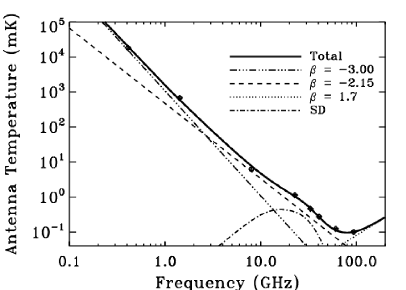
Figure 5.— Emission as a function of frequency in the $\delta=32^{\circ}$ strip, for observations in the range $0.4<\nu<94$ GHz relative to the 8 GHz observations. The emission is modeled as synchrotron, free-free, thermal dust, and spinning dust, with $\chi^{2}/{\rm dof}=12.8/3$, compared to $49.9/4$ when excluding spinning dust.

Table 3Foreground model for total emission along the $\delta=32^{\circ}$ Conklin strip

	Model 1		Model 2
	Nominal	Plus 6%	Nominal	Plus 6%
$a_{1}$	$-3.23\pm 0.12$	$-3.20\pm 0.12$	$-3.00\pm 0.12$	$-2.99\pm 0.11$
$\chi^{2}$/dof	47.2/4	39.7/4	11.6/3	8.8/3
$\Delta\chi^{2}$	…	…	35.6	30.9

4. Discussion

Anisotropy in the diffuse microwave emission at 8 GHz, originally measured by Conklin in 1969 to estimate the CMB dipole, now sheds light on Galactic emission. The observed signal is consistent with synchrotron, free-free, and spinning dust emission from the Galaxy. In combination with multi-frequency observations, the 8 GHz data strongly disfavor an emission model with no anomalous dust component, assumed to be rapidly rotating PAH grains. The presence of this additional diffuse component is consistent with observations by ARCADE-2, COSMOSOMAS, and the TENERIFE experiment, and with targeted measurements of dusty regions in the Galaxy. Accurate characterization of the Galactic foregrounds in intensity and polarization is important for extracting cosmological information from the CMB, and will be vital for constraining inflationary models via the large-scale polarization signal. Upcoming low-frequency observations, for example from the C-BASS experiment at 5 GHz (King et al., 2010), will shed further light on the diffuse anomalous dust behavior and allow its properties to be better established.

References

- Ali-Haïmoud et al. (2009) Ali-Haïmoud, Y., Hirata, C. M., & Dickinson, C. 2009, MNRAS, 395, 1055
- Banday et al. (2003) Banday, A. J., Dickinson, C., Davies, R. D., Davis, R. J., & Górski, K. M. 2003, MNRAS, 345, 897
- Battistelli et al. (2006) Battistelli, E. S., Rebolo, R., Rubiño-Martín, J. A., Hildebrandt, S. R., Watson, R. A., Gutiérrez, C., & Hoyland, R. J. 2006, ApJ, 645, L141
- Bennett et al. (2003) Bennett, C. L., et al. 2003, ApJS, 148, 97
- Bennett et al. (2003) Bennett, C. L., et al. 2003, ApJS, 148, 97
- Boughn & Pober (2007) Boughn, S. P. & Pober, J. C. 2007, ApJ, 661, 938
- Casassus et al. (2006) Casassus, S., Cabrera, G. F., Förster, F., Pearson, T. J., Readhead, A. C. S., & Dickinson, C. 2006, ApJ, 639, 951
- Casassus et al. (2004) Casassus, S., Readhead, A. C. S., Pearson, T. J., Nyman, L., Shepherd, M. C., & Bronfman, L. 2004, ApJ, 603, 599
- Casassus et al. (2008) Casassus, S., et al. 2008, MNRAS, 391, 1075
- Castellanos et al. (2011) Castellanos, P., et al. 2011, MNRAS, 411, 1137
- Conklin (1969a) Conklin, E. K. 1969a, Ph.D. thesis, Stanford University
- Conklin (1969b) —. 1969b, Nature, 222, 971
- Conklin (1972) Conklin, E. K. 1972, in IAU Symposium, Vol. 44, External Galaxies and Quasi-Stellar Objects, ed. D. S. Evans, D. Wills, & B. J. Wills, 518–+
- Conklin & Bracewell (1967) Conklin, E. K. & Bracewell, R. N. 1967, Nature, 216, 777
- Davies et al. (2006) Davies, R. D., Dickinson, C., Banday, A. J., Jaffe, T. R., Górski, K. M., & Davis, R. J. 2006, MNRAS, 370, 1125
- de Oliveira-Costa et al. (1997) de Oliveira-Costa, A., Kogut, A., Devlin, M. J., Netterfield, C. B., Page, L. A., & Wollack, E. J. 1997, ApJ, 482, L17+
- de Oliveira-Costa et al. (2004) de Oliveira-Costa, A., Tegmark, M., Davies, R. D., Gutiérrez, C. M., Lasenby, A. N., Rebolo, R., & Watson, R. A. 2004, ApJ, 606, L89
- de Oliveira-Costa et al. (2008) de Oliveira-Costa, A., Tegmark, M., Gaensler, B. M., Jonas, J., Landecker, T. L., & Reich, P. 2008, MNRAS, 388, 247
- de Oliveira-Costa et al. (1999) de Oliveira-Costa, A., Tegmark, M., Gutierrez, C. M., Jones, A. W., Davies, R. D., Lasenby, A. N., Rebolo, R., & Watson, R. A. 1999, ApJ, 527, L9
- de Oliveira-Costa et al. (1998) de Oliveira-Costa, A., Tegmark, M., Page, L. A., & Boughn, S. P. 1998, ApJ, 509, L9
- de Oliveira-Costa et al. (2002) de Oliveira-Costa, A. et al. 2002, ApJ, 567, 363
- Dickinson et al. (2009) Dickinson, C., et al. 2009, ApJ, 690, 1585
- Dickinson et al. (2010) —. 2010, MNRAS, 407, 2223
- Dobler et al. (2009) Dobler, G., Draine, B., & Finkbeiner, D. P. 2009, ApJ, 699, 1374
- Dobler & Finkbeiner (2008a) Dobler, G. & Finkbeiner, D. P. 2008a, ApJ, 680, 1222
- Dobler & Finkbeiner (2008b) —. 2008b, ApJ, 680, 1235
- Draine (2011) Draine, B. T. 2011, Personal communication via L. A. Page
- Draine & Lazarian (1998) Draine, B. T. & Lazarian, A. 1998, ApJ, 508, 157
- Draine & Lazarian (1999) —. 1999, ApJ, 512, 740
- Fernández-Cerezo et al. (2006) Fernández-Cerezo, S., et al. 2006, MNRAS, 370, 15
- Finkbeiner (2004) Finkbeiner, D. P. 2004, ApJ, 614, 186
- Finkbeiner et al. (1999) Finkbeiner, D. P., Davis, M., & Schlegel, D. J. 1999, ApJ, 524, 867
- Finkbeiner et al. (2004) Finkbeiner, D. P., Langston, G. I., & Minter, A. H. 2004, ApJ, 617, 350
- Finkbeiner et al. (2002) Finkbeiner, D. P., Schlegel, D. J., Frank, C., & Heiles, C. 2002, ApJ, 566, 898
- Gold et al. (2011) Gold, B., et al. 2011, ApJS, 192, 15
- Hamilton & Ganga (2001) Hamilton, J. & Ganga, K. M. 2001, A&A, 368, 760
- Haslam et al. (1981) Haslam, C. G. T., Klein, U., Salter, C. J., Stoffel, H., Wilson, W. E., Cleary, M. N., Cooke, D. J., & Thomasson, P. 1981, A&A, 100, 209
- Haslam et al. (1982) Haslam, C. G. T., Salter, C. J., Stoffel, H., & Wilson, W. E. 1982, A&AS, 47, 1, 2, 4
- Hildebrandt et al. (2007) Hildebrandt, S. R., Rebolo, R., Rubiño-Martín, J. A., Watson, R. A., Gutiérrez, C. M., Hoyland, R. J., & Battistelli, E. S. 2007, MNRAS, 382, 594
- Iglesias-Groth (2006) Iglesias-Groth, S. 2006, MNRAS, 368, 1925
- Jarosik et al. (2011) Jarosik, N., et al. 2011, ApJS, 192, 14
- Jones (1997) Jones, W. C. 1997, private communication. See also http://phy-page-g5.princeton.edu/page/
- King et al. (2010) King, O. G., et al. 2010, in Society of Photo-Optical Instrumentation Engineers (SPIE) Conference Series, Vol. 7741, Society of Photo-Optical Instrumentation Engineers (SPIE) Conference Series
- Kogut et al. (1996) Kogut, A., Banday, A. J., Bennett, C. L., Górski, K. M., Hinshaw, G., & Reach, W. T. 1996, ApJ, 460, 1
- Kogut et al. (2011) Kogut, A., et al. 2011, ApJ, 734, 4
- Lagache (2003) Lagache, G. 2003, A&A, 405, 813
- Leitch et al. (1997) Leitch, E. M., Readhead, A. C. S., Pearson, T. J., & Myers, S. T. 1997, ApJ, 486, L23
- Leitch et al. (2000) Leitch, E. M., Readhead, A. C. S., Pearson, T. J., Myers, S. T., Gulkis, S., & Lawrence, C. R. 2000, ApJ, 532, 37
- López-Caraballo et al. (2011) López-Caraballo, C. H., Rubiño-Martín, J. A., Rebolo, R., & Génova-Santos, R. 2011, ApJ, 729, 25
- Macellari et al. (2011) Macellari, N., Pierpaoli, E., Dickinson, C., & Vaillancourt, J. 2011, ArXiv e-prints
- Miville-Deschênes et al. (2008) Miville-Deschênes, M., Ysard, N., Lavabre, A., Ponthieu, N., Macías-Pérez, J. F., Aumont, J., & Bernard, J. P. 2008, A&A, 490, 1093
- Mukherjee et al. (2003) Mukherjee, P., Coble, K., Dragovan, M., Ganga, K., Kovac, J., Ratra, B., & Souradeep, T. 2003, ApJ, 592, 692
- Mukherjee et al. (2002) Mukherjee, P., Dennison, B., Ratra, B., Simonetti, J. H., Ganga, K., & Hamilton, J. 2002, ApJ, 579, 83
- Mukherjee et al. (2001) Mukherjee, P., Jones, A. W., Kneissl, R., & Lasenby, A. N. 2001, MNRAS, 320, 224
- Murphy et al. (2010) Murphy, E. J., et al. 2010, ApJ, 709, L108
- Pauliny-Toth & Shakeshaft (1962) Pauliny-Toth, I. K. & Shakeshaft, J. R. 1962, MNRAS, 124, 61
- Planck Collaboration et al. (2011) Planck Collaboration, et al. 2011, ArXiv e-prints
- Reich & Reich (1986) Reich, P. & Reich, W. 1986, A&AS, 63, 205
- Reich et al. (2001) Reich, P., Testori, J. C., & Reich, W. 2001, A&A, 376, 861
- Reich (1982) Reich, W. 1982, A&AS, 48, 219
- Scaife et al. (2009) Scaife, A. M. M., et al. 2009, MNRAS, 400, 1394
- Scaife et al. (2010a) —. 2010a, MNRAS, 403, L46
- Scaife et al. (2010b) —. 2010b, MNRAS, 406, L45
- Sletten (1988) Sletten, C. J. 1988, Reflector and Lens Antennas: Analysis and Design Using Personal Computers (Artech House, Incorporated), 65
- Tibbs et al. (2010) Tibbs, C. T., et al. 2010, MNRAS, 402, 1969
- Vidal et al. (2011) Vidal, M., et al. 2011, ArXiv e-prints
- Watson et al. (2005) Watson, R. A., Rebolo, R., Rubiño-Martín, J. A., Hildebrandt, S., Gutiérrez, C. M., Fernández-Cerezo, S., Hoyland, R. J., & Battistelli, E. S. 2005, ApJ, 624, L89
- Webster (1974) Webster, A. S. 1974, MNRAS, 166, 355
- Weingartner & Draine (2001) Weingartner, J. C. & Draine, B. T. 2001, ApJ, 548, 296
- Ysard et al. (2010) Ysard, N., Miville-Deschênes, M. A., & Verstraete, L. 2010, A&A, 509, L1+