The effect of small quenched noise on connectivity properties
of random interlacements

Abstract

Random interlacements (at level $u$) is a one parameter family of random subsets of ${\mathbb{Z}}^{d}$ introduced by Sznitman in [22]. The vacant set at level $u$ is the complement of the random interlacement at level $u$. While the random interlacement induces a connected subgraph of ${\mathbb{Z}}^{d}$ for all levels $u$, the vacant set has a non-trivial phase transition in $u$, as shown in [22] and [19].

In this paper, we study the effect of small quenched noise on connectivity properties of the random interlacement and the vacant set. For a positive $\varepsilon$, we allow each vertex of the random interlacement (referred to as occupied) to become vacant, and each vertex of the vacant set to become occupied with probability $\varepsilon$, independently of the randomness of the interlacement, and independently for different vertices. We prove that for any $d\geq 3$ and $u>0$, almost surely, the perturbed random interlacement percolates for small enough noise parameter $\varepsilon$. In fact, we prove the stronger statement that Bernoulli percolation on the random interlacement graph has a non-trivial phase transition in wide enough slabs. As a byproduct, we show that any electric network with i.i.d. positive resistances on the interlacement graph is transient, which strengthens our result in [17]. As for the vacant set, we show that for any $d\geq 3$, there is still a non-trivial phase transition in $u$ when the noise parameter $\varepsilon$ is small enough, and we give explicit upper and lower bounds on the value of the critical threshold, when $\varepsilon\to 0$.

1 Introduction

The model of random interlacements was recently introduced by Sznitman in [22] in order to describe the local picture left by the trajectory of a random walk on the discrete torus $({\mathbb{Z}}/N{\mathbb{Z}})^{d}$, $d\geq 3$ when it runs up to times of order $N^{d}$, or on the discrete cylinder $({\mathbb{Z}}/N{\mathbb{Z}})^{d}\times{\mathbb{Z}}$ , $d\geq 2$, when it runs up to times of order $N^{2d}$, see [20], [29]. Informally, the random interlacement Poisson point process consists of a countable collection of doubly infinite trajectories on ${\mathbb{Z}}^{d}$, and the trace left by these trajectories on a finite subset of ${\mathbb{Z}}^{d}$ “looks like” the trace of the above mentioned random walks.

The set of vertices visited by at least one of these trajectories is the random interlacement at level $u$ of Sznitman [22], and the complement of this set is the vacant set at level $u$. These are one parameter families of translation invariant, ergodic, long-range correlated random subsets of ${\mathbb{Z}}^{d}$, see [22]. We call the vertices of the random interlacement occupied, and the vertices of the vacant set vacant. While the set of occupied vertices induces a connected subgraph of ${\mathbb{Z}}^{d}$ for all levels $u$, the graph induced by the set of vacant vertices has a non-trivial phase transition in $u$, as shown in [22] and [19].

The effect of introducing a small amount of quenched disorder into a system with long-range correlations on the phase transition has got a lot of attention (see, e.g., [11], [28], [2], [3]). In this paper we consider how small quenched disorder affects the connectivity properties of the random interlacement and the vacant set. For $\varepsilon>0$, given a realization of the random interlacement, we allow each vertex independently to switch from occupied to vacant and from vacant to occupied with probability $\varepsilon$, and we study the effect it has on the existence of an infinite connected component in the graphs of occupied or vacant vertices.

We prove that for any $d\geq 3$ and $u>0$, almost surely, the set of occupied vertices percolates for small enough noise parameter $\varepsilon$. In fact, we prove the stronger statement that Bernoulli percolation on the random interlacement graph has a non-trivial phase transition in wide enough slabs. The two main ingredients of our proof are a strong connectivity lemma for the interlacement graph proved in [17] and Sznitman’s decoupling inequalities from [23]. As a byproduct, we show that any electric network with i.i.d. positive resistances on the interlacement graph is transient, which strengthens our result in [17].

We also prove that for any $d\geq 3$, the set of vacant vertices still undergoes a non-trivial phase transition in $u$ when the noise parameter $\varepsilon$ is small enough, and give explicit upper and lower bounds on the value of the threshold, when $\varepsilon\to 0$. The bounds that we derive suggest that the vacant set phase transition is robust with respect to noise, which we state as a conjecture.

1.1 The model

For $x\in{\mathbb{Z}}^{d}$, $d\geq 3$, let $P_{x}$ be the law of a simple random walk $X$ on ${\mathbb{Z}}^{d}$ with $X(0)=x$. Let $K$ be a finite subset of ${\mathbb{Z}}^{d}$. The equilibrium measure of $K$ is defined by

$$e_{K}(x)=P_{x}\left[X(t)\notin K~{}\mbox{for all}~{}t\geq 1\right],\quad\mbox{for }x\in K,\$$

and $e_{K}(x)=0$ for $x\notin K$. The capacity of $K$ is the total mass of the equilibrium measure of $K$:

$$\mathrm{cap}(K)=\sum_{x}e_{K}(x).\$$

Since $d\geq 3$, for any finite set $K\subset{\mathbb{Z}}^{d}$, the capacity of $K$ is positive. Therefore, we can define the normalized equilibrium measure by

$$\widetilde{e}_{K}(x)=e_{K}(x)/\mathrm{cap}(K).\$$

Let $W$ be the space of doubly-infinite nearest-neighbor trajectories in ${\mathbb{Z}}^{d}$ ($d\geq 3$) which tend to infinity at positive and negative infinite times, and let $W^{*}$ be the space of equivalence classes of trajectories in $W$ modulo time-shift. We write $\mathcal{W}$ for the canonical $\sigma$-algebra on $W$ generated by the coordinate maps, and $\mathcal{W}^{*}$ for the largest $\sigma$-algebra on $W^{*}$ for which the canonical map $\pi^{*}$ from $(W,\mathcal{W})$ to $(W^{*},\mathcal{W}^{*})$ is measurable.

Let $\mu$ be a Poisson point measure on $W^{*}$. For a finite subset $K$ of ${\mathbb{Z}}^{d}$, denote by $\mu_{K}$ the restriction of $\mu$ to the set of trajectories from $W^{*}$ that intersect $K$, and by $N_{K}$ be the number of trajectories in $\mathrm{Supp}(\mu_{K})$. The point measure $\mu_{K}$ can be written as $\mu_{K}=\sum_{i=1}^{N_{K}}\delta_{\pi^{*}(X_{i})}$, where $X_{i}$ are doubly-infinite trajectories from $W$ parametrized in such a way that $X_{i}(0)\in K$ and $X_{i}(t)\notin K$ for all $t<0$ and for all $i\in\{1,\ldots,N_{K}\}$.

For $u>0$, we say that a Poisson point measure $\mu$ on $W^{*}$ has distribution $\mathrm{Pois}(u,W^{*})$ if the following properties hold:

• The random variable $N_{K}$ has Poisson distribution with parameter $u\mathrm{cap}(K)$.

• Given $N_{K}$, the points $X_{i}(0)$, $i\in\{1,\ldots,N_{K}\}$, are independent and distributed according to the normalized equilibrium measure on $K$.

• Given $N_{K}$ and $(X_{i}(0))_{i=1}^{N_{K}}$, the corresponding forward and backward paths are conditionally independent, $(X_{i}(t),t\geq 0)_{i=1}^{N_{K}}$ are distributed as independent simple random walks, and $(X_{i}(t),t\leq 0)_{i=1}^{N_{K}}$ are distributed as independent random walks conditioned on not hitting $K$.

Properties (1)-(3) uniquely define $\mathrm{Pois}(u,W^{*})$, as proved in Theorem 1.1 in [22]. In fact, Theorem 1.1 in [22] gives a coupling of the Poisson point measures $\mu(u)$ with distribution $\mathrm{Pois}(u,W^{*})$ for all $u>0$. We refer the reader to [22] for more details.

Let $\mathbb{E}^{d}$ be the set of edges of ${\mathbb{Z}}^{d}$, i.e., $\mathbb{E}^{d}=\{\{x,y\}~{}:~{}x,y\in{\mathbb{Z}}^{d},|x-y|_{1}=1\}$. We will use the following convention throughout the paper. For a subset $J$ of $\mathbb{E}^{d}$, the subgraph of the lattice $({\mathbb{Z}}^{d},\mathbb{E}^{d})$ with the vertex set ${\mathbb{Z}}^{d}$ and the edge set $J$ will be also denoted by $J$.

For a Poisson point measure $\mu$ with distribution $\mathrm{Pois}(u,W^{*})$, the random interlacement $\mathcal{I}^{u}=\mathcal{I}^{u}(\mu)$ (at level $u$) is defined in [22] as the set of vertices of ${\mathbb{Z}}^{d}$ visited by at least one of the trajectories from $\mathrm{Supp}(\mu)$. This is a translation invariant and ergodic random subset of ${\mathbb{Z}}^{d}$, as shown in [22, Theorem 2.1]. The law of $\mathcal{I}^{u}$ is characterized by the identity (see (0.10) and Remark 2.2 (2) in [22]):

$$\mathbb{P}\left[\mathcal{I}^{u}\cap K=\emptyset\right]=e^{-u\mathrm{cap}(K)},\quad\text{for all finite $K\subseteq{\mathbb{Z}}^{d}$}.\$$

We denote by ${\widetilde{\mathcal{I}}}^{u}={\widetilde{\mathcal{I}}}^{u}(\mu)$ the set of edges of $\mathbb{E}^{d}$ traversed by at least one of the trajectories from $\mathrm{Supp}(\mu)$. The corresponding random subgraph ${\widetilde{\mathcal{I}}}^{u}$ of $({\mathbb{Z}}^{d},\mathbb{E}^{d})$ (with the vertex set ${\mathbb{Z}}^{d}$ and the edge set ${\widetilde{\mathcal{I}}}^{u}$) is called the random interlacement graph (at level $u$). It follows from Theorem 2.1 and Remark 2.2(4) of [22] that ${\widetilde{\mathcal{I}}}^{u}$ is a translation invariant ergodic random subgraph of $({\mathbb{Z}}^{d},\mathbb{E}^{d})$. Let $\mathcal{V}^{u}={\mathbb{Z}}^{d}\setminus\mathcal{I}^{u}$ be the vacant set at level $u$.

Given a parameter $\varepsilon\in(0,1)$, we consider the family $\theta_{x}$, $x\in{\mathbb{Z}}^{d}$, of independent Bernoulli random variables (an independent noise) with parameter $\varepsilon$, and define $\varepsilon$-disordered analogues of the random interlacement $\mathcal{I}^{u,\varepsilon}$ and the vacant set $\mathcal{V}^{u,\varepsilon}$ as follows. We say that $x\in\mathcal{I}^{u,\varepsilon}$ if $x\in\mathcal{I}^{u}$ and $\theta_{x}=0$ or $x\in\mathcal{V}^{u}$ and $\theta_{x}=1$. In other words, the vertices of the random interlacement get an $\varepsilon$-chance to become vacant, and the vertices of the vacant set get an $\varepsilon$-chance to become occupied. Let $\mathcal{V}^{u,\varepsilon}={\mathbb{Z}}^{d}\setminus\mathcal{I}^{u,\varepsilon}$. We are interested in percolative properties of $\mathcal{I}^{u,\varepsilon}$ and $\mathcal{V}^{u,\varepsilon}$. It follows from Remark 1.6(4) in [22] that for any $d\geq 3$ and $u>0$,

$$\mbox{cov}_{u}\left[\mathds{1}(x\in\mathcal{V}^{u}),\mathds{1}(y\in\mathcal{V}^{u})\right]\asymp\left(1+|x-y|_{\infty}\right)^{2-d},\quad\mbox{for }x,y\in{\mathbb{Z}}^{d},\$$

where $\mbox{cov}_{u}$ denotes the covariance under $\mathrm{Pois}(u,W^{*})$. This displays the presence of long-range correlations in $\mathcal{V}^{u}$. Non-rigorous study of the effect of small quenched noise on the critical behavior of a system with long-range correlations was initiated in [11, 28].

It was shown, among other results, in [22] that the random interlacement graph ${\widetilde{\mathcal{I}}}^{u}$ consists of a unique infinite connected component and isolated vertices. (Refinements of this result were obtained in [12, 15, 16].) In [17], we showed that the random interlacement graph is almost surely transient for any $u>0$ in dimensions $d\geq 3$. In Theorem 1 of the present paper, we prove that for any $u>0$ and small enough $\varepsilon>0$, the set $\mathcal{I}^{u,\varepsilon}$ still contains an infinite connected component. In fact, Theorem 1 implies that $\mathcal{I}^{u}$ and ${\widetilde{\mathcal{I}}}^{u}$ still have an infinite connected component in wide enough slabs, even after a small positive density of vertices of $\mathcal{I}^{u}$, respectively edges of ${\widetilde{\mathcal{I}}}^{u}$, is removed. One might interpret all these results as an evidence of the heuristic statement that the geometry of the interlacement graph is similar to that of the underlying lattice ${\mathbb{Z}}^{d}$. Recently, this question has been settled in [4] by a clever refinement of the techniques in [16, 17]. It was proved in [4] (and later in [8] with a different, model independent proof) that the graph distance in $\mathcal{I}^{u}$ is comparable to the graph distance in ${\mathbb{Z}}^{d}$, and a shape theorem holds for balls with respect to graph distance on $\mathcal{I}^{u}$. First results about heat-kernel bounds for the random walk on $\mathcal{I}^{u}$ have been recently obtained in [14, Theorem 2.3].

An important role in understanding the local picture left by the trajectory of a random walk on the discrete torus $({\mathbb{Z}}/N{\mathbb{Z}})^{d}$, $d\geq 3$ or the discrete cylinder $({\mathbb{Z}}/N{\mathbb{Z}})^{d}\times{\mathbb{Z}}$ , $d\geq 2$ is played by

$$u_{*}=\inf\{u\geq 0\;:\;\mathbb{P}[0\leftrightarrow\infty\mbox{ in }\mathcal{V}^{u}]=0\}$$

(see, e.g., [21, 26]). It follows from [22, (1.53) and (1.55)] that for $u<u^{\prime}$, the set $\mathcal{V}^{u^{\prime}}$ is stochastically dominated by $\mathcal{V}^{u}$. Therefore, for all $u>u_{*}$, $\mathbb{P}[0\leftrightarrow\infty\mbox{ in }\mathcal{V}^{u}]=0$. Moreover, by [19, 22], $u_{*}\in(0,\infty)$, i.e., there is a non-trivial phase transition for $\mathcal{V}^{u}$ in $u$ at $u_{*}$. In Theorem 3 of this paper, we prove that for small enough $\varepsilon$, the $\varepsilon$-disordered vacant set $\mathcal{V}^{u,\varepsilon}$ still undergoes a non-trivial phase transition in $u$. In Theorem 5 we give explicit upper and lower bounds on the phase transition threshold for $\mathcal{V}^{u,\varepsilon}$, as $\varepsilon\to 0$. These bounds suggest that the phase transition is actually robust with respect to noise. We state it as a conjecture in Remark 3.

2 Main results

For $p\in(0,1)$, we define the random subset ${\widetilde{\mathcal{B}}}^{p}$ of $\mathbb{E}^{d}$ by deleting each edge with probability $(1-p)$ and retaining it with probability $p$, independently for all edges, and, similarly, the random subset $\mathcal{B}^{p}$ of ${\mathbb{Z}}^{d}$ by deleting every vertex of ${\mathbb{Z}}^{d}$ with probability $(1-p)$ and retaining it with probability $p$, independently for all vertices. We look at the random subgraphs of $({\mathbb{Z}}^{d},\mathbb{E}^{d})$ with vertex set ${\mathbb{Z}}^{d}$ and edge set ${\widetilde{\mathcal{I}}}^{u}\cap{\widetilde{\mathcal{B}}}^{p}$, and the one induced by the set of vertices $\mathcal{I}^{u}\cap\mathcal{B}^{p}\subset{\mathbb{Z}}^{d}$.

Our first theorem states that the graphs $\mathcal{I}^{u}$ and ${\widetilde{\mathcal{I}}}^{u}$ have infinite connected subgraphs in a wide enough slab, moreover, Bernoulli bond percolation on ${\widetilde{\mathcal{I}}}^{u}$ and Bernoulli site percolation on $\mathcal{I}^{u}$ restricted to this slab have a non-trivial phase transition.

Theorem 1.

Let $d\geq 3$ and $u>0$. There exist $p<1$ and $R\geq 1$ such that, almost surely, the random graphs $\mathcal{I}^{u}\cap\mathcal{B}^{p}$ and ${\widetilde{\mathcal{I}}}^{u}\cap{\widetilde{\mathcal{B}}}^{p}$ contain infinite connected components in the slab ${\mathbb{Z}}^{2}\times[0,R)^{d-2}$.

As a byproduct of the proof of Theorem 1, we obtain the following generalization of the main result in [17].

Theorem 2.

Let $d\geq 3$ and $u>0$. Let $R_{{\widetilde{e}}}$, ${\widetilde{e}}\in\mathbb{E}^{d}$ be independent identically distributed positive random variables. The electric network $\{{\widetilde{e}}~{}:~{}{\widetilde{e}}\in{\widetilde{\mathcal{I}}}^{u}\}$ with resistances $R_{{\widetilde{e}}}$ is almost surely transient, i.e., the effective resistance between any vertex in ${\widetilde{\mathcal{I}}}^{u}$ and infinity is finite.

Theorem 2 is a generalization of the main result of [17], since the transience of the unique infinite connected component of the random interlacement graph ${\widetilde{\mathcal{I}}}^{u}$ follows from the case when $R_{{\widetilde{e}}}$ are almost surely equal to $1$ (see, e.g., [6]). The result of Theorem 2 is equivalent (see the main result of [13]) to the following statement: for any $u>0$, there exists $p<1$ such that the graph ${\widetilde{\mathcal{I}}}^{u}\cap{\widetilde{\mathcal{B}}}^{p}$ contains a transient component, i.e., the simple random walk on it is transient. The proof of this fact will come as a byproduct of the proof of Theorem 1.

The main idea of the proofs of Theorems 1 and 2 is renormalization. We partition the graph ${\mathbb{Z}}^{d}$ into disjoint blocks of equal size. A block is called good if the graph ${\widetilde{\mathcal{I}}}^{u}$ contains a unique large connected component in this block and all the edges of the block are in ${\widetilde{\mathcal{B}}}^{p}$, otherwise it is called bad. A more precise definition will be given in Section 5. It will be shown that paths of good blocks contain paths of ${\widetilde{\mathcal{I}}}^{u}\cap{\widetilde{\mathcal{B}}}^{p}$. In particular, percolation of good blocks implies percolation of ${\widetilde{\mathcal{I}}}^{u}\cap{\widetilde{\mathcal{B}}}^{p}$. Using the strong connectivity result of [17], stated as Lemma 1 below, we show that a block is good with probability tending to $1$, as the size of the block increases. We then use the decoupling inequalities of [23], stated as Theorem 4 below, to show in Lemma 6 that $*$-connected components of bad blocks are small. With the result of Lemma 6, the existence statement of Theorem 1 follows using a standard duality argument, and the proof of Theorem 2 is reminiscent of the proof of Theorem 1 in Section 3 of [17].

In our next theorem, we show that for small enough $\varepsilon>0$, the $\varepsilon$-disordered vacant set $\mathcal{V}^{u,\varepsilon}$ undergoes a non-trivial phase transition in $u$. Let

$$u_{*}(\varepsilon)=\inf\{u\geq 0\;:\;\mathbb{P}[0\leftrightarrow\infty\mbox{ in }\mathcal{V}^{u,\varepsilon}]=0\}.\$$

Theorem 3.

Let $d\geq 3$. For any $\varepsilon\in(0,1/2)$ and $u>u_{*}(\varepsilon)$,

$$\mathbb{P}[0\leftrightarrow\infty\mbox{ in }\mathcal{V}^{u,\varepsilon}]=0.\$$

In other words, for $\varepsilon\in(0,1/2)$, the $\varepsilon$-disordered vacant set $\mathcal{V}^{u,\varepsilon}$ undergoes a phase transition in $u$ at $u_{*}(\varepsilon)$. Moreover, there exists $\varepsilon_{0}>0$ such that for all $\varepsilon\leq\varepsilon_{0}$,

$$0<u_{*}(\varepsilon)<\infty.\$$

The first statement of Theorem 3 is proved in Lemma 7. It follows from a standard coupling argument and the fact that the set $\mathcal{V}^{u^{\prime}}$ is stochastically dominated by $\mathcal{V}^{u}$ for $u<u^{\prime}$ (see [22, (1.53) and (1.55)]). The second statement of Theorem 3 follows from the more general statement of Theorem 5, in which we give explicit upper and lower bounds on $u_{*}(\varepsilon)$, as $\varepsilon\to 0$. The proof of Theorem 5 uses renormalization, and is very similar in spirit to the proof of Theorem 1.

The bounds on $u_{*}(\varepsilon)$ that we obtain in Theorem 5 are in terms of certain thresholds describing local behavior of $\mathcal{V}^{u}$ in sub- and supercritical regimes (see (7.4) and Definition 7.1, respectively). In particular, they are purely in terms of $\mathcal{V}^{u}$ and not $\mathcal{V}^{u,\varepsilon}$. As we discuss in Remark 3, these thresholds are conjectured to coincide with $u_{*}$, therefore it is reasonable to believe that the phase transition of $\mathcal{V}^{u}$ is stable with respect to small random noise. In other words, the following conjecture holds:

$$\lim_{\varepsilon\to 0}u_{*}(\varepsilon)=u_{*}.\$$

Finally, note that it is essential for $u_{*}(\varepsilon)<\infty$ that the parameter $\varepsilon$ is small. For example, since $\mathcal{V}^{u,1/2}$ has the same law as the Bernoulli site percolation with parameter $1/2$, which is supercritical in dimensions $d\geq 3$ (see [1]), we obtain that $u_{*}(1/2)=\infty$.

We now describe the structure of the remaining sections of the paper. We recall the strong connectivity lemma of [17] and the decoupling inequalities of [23] in Section 3. In Section 4 we construct and study seed events which are used in Section 5 to define good blocks. Lemma 6, the main ingredient of the proofs of Theorems 1 and 2, is proved in Section 5. The proofs of Theorems 1 and 2 are given in Section 6, and the proof of Theorem 3 is given in Section 7, where we also give explicit bounds on $u_{*}(\varepsilon)$, as $\varepsilon\to 0$.

3 Notation and known results

In this section we introduce basic notation and collect some properties of the random interlacements, which are recurrently used in our proofs.

3.1 Notation

For $a\in{\mathbb{R}}$, we write $|a|$ for the absolute value of $a$, and $\lfloor a\rfloor$ for the integer part of $a$. For $(x_{1},\dots,x_{d})=x\in{\mathbb{Z}}^{d}$, we write $|x|_{\infty}$ for the $l^{\infty}$-norm of $x$, i.e., $|x|_{\infty}=\max\left(|x_{1}|,\ldots,|x_{d}|\right)$, and $|x|_{1}$ for the $l^{1}$-norm of $x$, i.e., $|x|_{1}=\sum_{i=1}^{d}|x_{i}|$. For $R>0$ and $x\in{\mathbb{Z}}^{d}$, let $B(x,R)=\{y\in{\mathbb{Z}}^{d}~{}:~{}|x-y|_{\infty}\leq R\}$ be the $l^{\infty}$-ball of radius $R$ centered at $x$, and $B(R)=B(0,R)$.

For $x\in{\mathbb{Z}}^{d}$ and integers $m<n$, we write $x+[m,n)^{d}$ for the set of vertices $y=(y_{1},\ldots,y_{d})\in{\mathbb{Z}}^{d}$ with $m\leq y_{i}-x_{i}<n$ for all $i\in\{1,\ldots,d\}$. For ${\widetilde{e}}\in\mathbb{E}^{d}$, we write ${\widetilde{e}}\in x+[m,n)^{d}$ if both of its endvertices are in $x+[m,n)^{d}$. If ${\widetilde{J}}\subseteq\mathbb{E}^{d}$, we denote by ${\widetilde{J}}\cap(x+[m,n)^{d})$ the set of edges of ${\widetilde{J}}$ with both endvertices in $x+[m,n)^{d}$. For $x,y\in{\mathbb{Z}}^{d}$, we write $x\leftrightarrow y$ in ${\widetilde{J}}$, if $x$ and $y$ are in the same connected component of the graph ${\widetilde{J}}$.

Let $(\Omega_{1},\mathcal{F}_{1},\mathbb{P}^{u})$, with $\Omega_{1}=\{0,1\}^{\mathbb{E}^{d}}$ and the canonical $\sigma$-algebra $\mathcal{F}_{1}$, be the probability space on which ${\widetilde{\mathcal{I}}}^{u}$ is defined. For $\omega\in\Omega_{1}$, we say that ${\widetilde{e}}\in\mathbb{E}^{d}$ is in ${\widetilde{\mathcal{I}}}^{u}$ when $\omega_{\widetilde{e}}=1$. Let $(\Omega_{2},\mathcal{F}_{2},\mathbf{P}_{p})$, with $\Omega_{2}=\{0,1\}^{\mathbb{E}^{d}}$ and the canonical $\sigma$-algebra $\mathcal{F}_{2}$, be the probability space on which ${\widetilde{\mathcal{B}}}^{p}$ is defined. For $\omega\in\Omega_{2}$, we say that ${\widetilde{e}}\in\mathbb{E}^{d}$ is in ${\widetilde{\mathcal{B}}}^{p}$ when $\omega_{\widetilde{e}}=1$. Finally, let $(\Omega,\mathcal{F},\mathbb{P})=(\Omega_{1}\times\Omega_{2},\mathcal{F}_{1}\times\mathcal{F}_{2},\mathbb{P}^{u}\otimes\mathbf{P}_{p})$ denote the probability space on which the random interlacement graph ${\widetilde{\mathcal{I}}}^{u}$ and Bernoulli bond percolation configuration ${\widetilde{\mathcal{B}}}^{p}$ are jointly defined.

Throughout the paper, we use the following notational agreement. For events $A_{1}\in\mathcal{F}_{1}$ and $A_{2}\in\mathcal{F}_{2}$, we denote the corresponding events $A_{1}\times\Omega_{2}$ and $\Omega_{1}\times A_{2}$ in $\mathcal{F}$ also by $A_{1}$ and $A_{2}$, respectively. We denote by $\mathds{1}(A)$ the indicator of event $A$ and by $A^{c}$ the complement of $A$. For $i\in\{1,2\}$, given a random subset ${\widetilde{\mathcal{J}}}(\omega)$ of $\mathbb{E}^{d}$, with $\omega\in\Omega_{i}$, and an event $A\in\mathcal{F}_{i}$, we define

$$A({\widetilde{\mathcal{J}}})=\{\omega\in\Omega_{i}~{}:~{}\chi_{{\widetilde{\mathcal{J}}}(\omega)}\in A\},\$$ (3.1)

where for ${\widetilde{e}}\in\mathbb{E}^{d}$, $\chi_{{\widetilde{\mathcal{J}}}(\omega)}({\widetilde{e}})$ equals $1$ if ${\widetilde{e}}\in{\widetilde{\mathcal{J}}}(\omega)$, and $0$ otherwise. Conversely, for an element $\omega\in\{0,1\}^{\mathbb{E}^{d}}$, let

$$G_{\omega}=\{{\widetilde{e}}~{}:~{}\omega_{\widetilde{e}}=1\}.\$$ (3.2)

(By our convention, we also denote by $G_{\omega}$ the graph with the vertex set ${\mathbb{Z}}^{d}$ and the edge set $\{{\widetilde{e}}~{}:~{}\omega_{\widetilde{e}}=1\}$.) An event $A\in\mathcal{F}_{1}$ is called increasing, if for any $\omega\in A$, all the elements $\omega^{\prime}$ with $G_{\omega^{\prime}}\supseteq G_{\omega}$ are in $A$. The event $A$ is called decreasing, if $A^{c}$ is increasing. Throughout the text, we write $c$ and $C$ for small positive and large finite constants, respectively, that may depend on $d$ and $u$. Their values may change from place to place.

3.2 Strong connectivity property

The following strong connectivity lemma follows from Proposition 1 in [17].

Lemma 1.

Let $d\geq 3$, $u>0$, and $\varepsilon>0$. There exist constants $c=c(d,u,\varepsilon)>0$ and $C=C(d,u,\varepsilon)<\infty$ such that for all $R\geq 1$,

$$\mathbb{P}\left[\bigcap_{x,y\in\mathcal{I}^{u}\cap[0,R)^{d}}\left\{x\leftrightarrow y\quad\mbox{in}\quad{\widetilde{\mathcal{I}}}^{u}\cap[-\varepsilon R,(1+\varepsilon)R)^{d}\right\}\right]\geq 1-C\exp(-cR^{1/6}).\$$

Lemma 1 may seem more general than Proposition 1 in [17], but, in fact, the two results are equivalent. In order to see this, the reader may check how Proposition 1 is derived from Lemma 13 in [17].

3.3 Decoupling inequalities

Let

$$l(d)=30\cdot 4^{d}.\$$ (3.3)

(The choice of $l(d)$ will be justified in the proof of Lemma 6.) Let $L_{0}$ and $l_{0}\geq l(d)$ be positive integers. We introduce the geometrically increasing sequence of length scales

$$L_{n}=l_{0}^{n}L_{0},\qquad n\geq 1.$$

For $n\geq 0$, we introduce the renormalized lattice graph $\mathbb{G}_{n}$ by

$$\mathbb{G}_{n}=L_{n}{\mathbb{Z}}^{d}=\{L_{n}x~{}:~{}x\in{\mathbb{Z}}^{d}\}.\$$

For $x\in\mathbb{G}_{n}$ and $n\geq 0$, let

$$\Lambda_{x,n}=\mathbb{G}_{n-1}\cap(x+[0,L_{n})^{d}).\$$

Let $\Psi_{{\widetilde{e}}},{\widetilde{e}}\in\mathbb{E}^{d}$ denote the canonical coordinates on $\{0,1\}^{\mathbb{E}^{d}}$. For $x\in\mathbb{G}_{0}$, let ${\overline{G}}_{x}={\overline{G}}_{x,0}={\overline{G}}_{x,0,L_{0}}$ be a $\sigma(\Psi_{{\widetilde{e}}},{\widetilde{e}}\in x+[-L_{0},3L_{0})^{d})$-measurable event. We call events of the form ${\overline{G}}_{x,0,L_{0}}$ seed events. We denote the family of events $({\overline{G}}_{x,0,L_{0}}~{}:~{}L_{0}\geq 1,x\in\mathbb{G}_{0})$ by ${\overline{G}}$. Examples of seed events important for this paper will be considered in Section 4. The reader should think about the events ${\overline{G}}_{x,0,L_{0}}$ as “bad” events. Now we recursively define bad events on higher length scales using seed events. For $n\geq 1$ and $x\in{\mathbb{Z}}^{d}$, denote by ${\overline{G}}_{x,n}={\overline{G}}_{x,n,L_{0}}$ the event that there exist $x_{1},x_{2}\in\Lambda_{x,n}$ with $|x_{1}-x_{2}|_{\infty}>L_{n}/l(d)$ such that the events ${\overline{G}}_{x_{1},n-1}$ and ${\overline{G}}_{x_{2},n-1}$ occur:

$${\overline{G}}_{x,n}=\bigcup_{x_{1},x_{2}\in\Lambda_{x,n};\,|x_{1}-x_{2}|_{\infty}>\frac{L_{n}}{l(d)}}{\overline{G}}_{x_{1},n-1}\cap{\overline{G}}_{x_{2},n-1}\quad.\$$ (3.4)

(For simplicity, we omit the dependence of ${\overline{G}}_{x,n}$ on $L_{0}$ from the notation.) Note that ${\overline{G}}_{x,n}$ is $\sigma(\Psi_{{\widetilde{e}}},{\widetilde{e}}\in x+[-L_{n},3L_{n})^{d})$-measurable. (This can be shown by induction on $n$.)

Recall the definition (3.1). The following theorem is a special case of Theorem 3.4 in [23] (modulo some minor changes that we explain in the proof).

Theorem 4.

For all $d\geq 3$, $u>0$ and $\delta\in(0,1)$, there exists $C=C(d,u,\delta)<\infty$ such that for all $n\geq 0$, $L_{0}\geq 1$, and $l_{0}\geq C$ a multiple of $l(d)$, we have

1. if ${\overline{G}}_{x}$ are decreasing events, then for all $u^{\prime}\geq(1+\delta)u$,

   $$\mathbb{P}\left[{\overline{G}}_{0,n}({\widetilde{\mathcal{I}}}^{u^{\prime}})\right]\leq\left(l_{0}^{2d}\sup_{x\in\mathbb{G}_{0}\cap[0,L_{n})^{d}}\mathbb{P}\left[{\overline{G}}_{x}({\widetilde{\mathcal{I}}}^{u})\right]+\frac{1}{4}\right)^{2^{n}},\$$ (3.5)

2. if ${\overline{G}}_{x}$ are increasing events, then for all $u^{\prime}\leq(1-\delta)u$,

   $$\mathbb{P}\left[{\overline{G}}_{0,n}({\widetilde{\mathcal{I}}}^{u^{\prime}})\right]\leq\left(l_{0}^{2d}\sup_{x\in\mathbb{G}_{0}\cap[0,L_{n})^{d}}\mathbb{P}\left[{\overline{G}}_{x}({\widetilde{\mathcal{I}}}^{u})\right]+\frac{1}{4}\right)^{2^{n}}.\$$ (3.6)

Proof of Theorem 4.

We refer the reader to Section 3 of [23] for the notation. Our events ${\overline{G}}_{x,n}$ correspond to the events $G_{x,L_{n}}$ of [23], $\Lambda_{x,n}$ plays the role of $\Lambda$, thus $c(\mathcal{G},l)=1$ and $\lambda=d$ in Definition 3.1 of [23]. There are a number of comments we would like to make before applying results derived in Section 3 of [23]:

(1) Even though the events $G_{x,L_{n}}$ in [23] pertain to the occupancy of vertices (i.e., they are subsets of $\{0,1\}^{{\mathbb{Z}}^{d}}$), Theorem 3.4 in [23] also applies in the setting when the events $G_{x,L_{n}}$ pertain to the occupancy of edges (i.e., they are subsets of $\{0,1\}^{\mathbb{E}^{d}}$), see Theorem 2.1, Remark 2.5(3) and Corollary 2.1’ of [23].

(2) The constant $l(d)$ is taken to be $100$ in Definition 3.1 in [23], but Theorem 3.4 in [23] works for any large enough constant $l(d)$, with $l_{0}>l(d)$ also large enough.

(3) The events ${\overline{G}}_{x,n}$ defined by (3.4) are not cascading in the sense of Definition 3.1 in [23], because $(3.4)$ of [23] only holds for $l=l_{0}$ rather than for all $l$ which is a multiple of $100$. Nevertheless, the statement and the proof of Theorem 3.4 in [23] only involve events $G_{x,L_{n}}$, with $L_{n}=l_{0}^{n}L_{0}$ for some previously fixed $L_{0}\geq 1$ and $l_{0}$ (where $l_{0}$ is large enough).

Taking the above remarks into account, we can apply Theorem 3.4 of [23] to the events ${\overline{G}}_{x,n}$. In order to derive (3.5) and (3.6) from Theorem 3.4 of [23], we choose $l_{0}$ large enough, so that $u_{\infty}^{+}\leq(1+\delta)u$, $u_{\infty}^{-}\geq(1-\delta)u$, and $l_{0}^{2d}\varepsilon(u_{\infty}^{-})\leq 1/4$. (See, e.g., the calculations in (3.37) of [23].) ∎

Remark 1.

Currently, Theorem 3.4 in [23] (and, as a result, Theorem 4 of this paper) is proved only for increasing and decreasing events. It would be interesting to show that the result of Theorem 3.4 in [23] holds for a more general class of events.

Corollary 1.

Let $d\geq 3$, $u>0$ and $\delta\in(0,1)$. Let ${\overline{G}}_{x}$ be all increasing events and $u^{\prime}=(1-\delta)u$, or all decreasing events and $u^{\prime}=(1+\delta)u$. If

$$\liminf_{L_{0}\to\infty}\sup_{x\in\mathbb{G}_{0}\cap[0,L_{n})^{d}}\mathbb{P}\left[{\overline{G}}_{x}({\widetilde{\mathcal{I}}}^{u})\right]=0,\$$ (3.7)

then there exist $l_{0},L_{0}\geq 1$ such that for all $n\geq 0$,

$$\mathbb{P}\left[{\overline{G}}_{0,n}({\widetilde{\mathcal{I}}}^{u^{\prime}})\right]\leq 2^{-2^{n}}.\$$ (3.8)

Moreover, if the limit in (3.7) (as $L_{0}\to\infty$) exists and equals to $0$, then there exists $C=C(d,u,\delta)<\infty$ such that the inequality (3.8) holds for all $l_{0}\geq C$ a multiple of $l(d)$, $L_{0}\geq C^{\prime}(d,u,\delta,l_{0},{\overline{G}})$ (for some constant $C^{\prime}(d,u,\delta,l_{0},{\overline{G}})$), and $n\geq 0$.

4 Seed events

In this section we apply Corollary 1 to two families of (decreasing and increasing) bad events defined in terms of ${\widetilde{\mathcal{I}}}^{u}$. We also recursively define a similar (but simpler) family of bad events in terms of ${\widetilde{\mathcal{B}}}^{p}$ and derive results analogous to Corollary 1 for this family given that $p$ is close enough to $1$. The corresponding seed events will be used in Section 5 to define good vertices in $\mathbb{G}_{0}$. The good vertices will have the property that the existence of an infinite path of good vertices in $\mathbb{G}_{0}$ implies the existence of an infinite path in the graph ${\widetilde{\mathcal{I}}}^{u}\cap{\widetilde{\mathcal{B}}}^{p}$, as stated formally in Lemma 5.

We define the density of the interlacement at level $u$ (see, e.g., (1.58) in [22]) by

$$m(u)=\mathbb{P}(0\in\mathcal{I}^{u})=1-e^{-u/g(0)},\$$

where $g$ is the Green function of the simple random walk on ${\mathbb{Z}}^{d}$ started at $0$. The function $m$ is continuous.

Note that $x\in\mathcal{I}^{u}$ if and only if $\{x,y\}\in{\widetilde{\mathcal{I}}}^{u}$ for some $y\in{\mathbb{Z}}^{d}$, thus $\mathcal{I}^{u}$ is a measurable function of ${\widetilde{\mathcal{I}}}^{u}$. It follows from Theorem 2.1 and Remark 2.2(4) of [22] that ${\widetilde{\mathcal{I}}}^{u}$ is a translation invariant ergodic random subset of $\mathbb{E}^{d}$. By an appropriate ergodic theorem (see, e.g., Theorem VIII.6.9 in [9]), we get

$$\lim_{L\to\infty}\frac{1}{L^{d}}\sum_{x\in[0,L)^{d}}\mathds{1}\left(\,\exists y\in[0,L)^{d}\,:\;\{x,y\}\in{\widetilde{\mathcal{I}}}^{u}\,\right)\;\stackrel{{\scriptstyle\mathbb{P}\text{-a.s.}}}{{=}}\;m(u).$$ (4.1)

4.1 Bad decreasing events

In this subsection we define and study a family of bad decreasing $\sigma(\Psi_{\widetilde{e}},~{}{\widetilde{e}}\in x+[0,2L_{n})^{d})$-measurable events $\overline{E}_{x,n}^{u}$ with (see (3.4))

$$\overline{E}_{x,n}^{u}=\bigcup_{x_{1},x_{2}\in\Lambda_{x,n};\,|x_{1}-x_{2}|_{\infty}>\frac{L_{n}}{l(d)}}\overline{E}_{x_{1},n-1}^{u}\cap\overline{E}_{x_{2},n-1}^{u}\quad,\$$

for $n\geq 1$, and $\mathbb{P}\left[\overline{E}_{0,n}^{u}({\widetilde{\mathcal{I}}}^{u})\right]\leq 2^{-2^{n}}$. In order to define the bad decreasing seed event $\overline{E}_{x}^{u}=\overline{E}_{x,0}^{u}$, we define its complement, the “good” increasing event $E_{x}^{u}=(\overline{E}_{x}^{u})^{c}$.

Definition 4.1.

Fix $u>0$. Recall the definition of the graph $G_{\omega}$ in (3.2). Let $E_{x}^{u}$ be the measurable subset of $\{0,1\}^{\mathbb{E}^{d}}$ such that $\omega\in E_{x}^{u}$ iff

1. for all $e\in\{0,1\}^{d}$, the graph $G_{\omega}\cap(x+eL_{0}+[0,L_{0})^{d})$ contains a connected component with at least $\frac{3}{4}m(u)L_{0}^{d}$ vertices,

2. all of these $2^{d}$ components are connected in the graph $G_{\omega}\cap(x+[0,2L_{0})^{d})$.

Note that $E_{x}^{u}$ is an increasing $\sigma(\Psi_{\widetilde{e}},~{}{\widetilde{e}}\in x+[0,2L_{0})^{d})$-measurable event. Moreover, if ${\widetilde{\mathcal{J}}}(\omega)$ is a random translation invariant subset of $\mathbb{E}^{d}$, then $\mathbb{P}[E_{x}^{u}({\widetilde{\mathcal{J}}})]=\mathbb{P}[E_{0}^{u}({\widetilde{\mathcal{J}}})]$ for all $x\in{\mathbb{Z}}^{d}$.

Lemma 2.

For any $u>0$ there exists $\delta>0$ such that

$$\mathbb{P}[E_{0}^{u}({\widetilde{\mathcal{I}}}^{u/(1+\delta)})]\to 1,\quad\mbox{as}\quad L_{0}\to\infty.\$$ (4.2)

Proof of Lemma 2.

Let $u>0$. By the continuity of $m(u)$, we can choose $\varepsilon>0$ and $\delta>0$ so that

$$(1-4\varepsilon)^{d}m\left(\frac{u}{1+\delta}\right)>\frac{3}{4}m(u).\$$

With such a choice of $\varepsilon$ and $\delta$, for $L_{0}\geq 1$, we obtain

$$m\left(\frac{u}{1+\delta}\right)(L_{0}-4\lfloor\varepsilon L_{0}\rfloor)^{d}>\frac{3}{4}m(u)L_{0}^{d}.\$$ (4.3)

Let $u^{\prime}=u/(1+\delta)$. We consider the boxes

$$B_{e}=eL_{0}+[\,2\lfloor\varepsilon L_{0}\rfloor,L_{0}-2\lfloor\varepsilon L_{0}\rfloor\,)^{d},\qquad e\in\{0,1\}^{d}.$$

The volume of $B_{e}$ is $|B_{e}|=(L_{0}-4\lfloor\varepsilon L_{0}\rfloor)^{d}$. Using (4.1) and (4.3), we get that with probability tending to $1$ as $L_{0}\to\infty$, each of the boxes $B_{e}$, $e\in\{0,1\}^{d}$ contains at least $\frac{3}{4}m(u)L_{0}^{d}$ vertices of $\mathcal{I}^{u^{\prime}}$.

Now by Lemma 1, all the vertices of $\mathcal{I}^{u^{\prime}}\cap B_{e}$ are connected in ${\widetilde{\mathcal{I}}}^{u^{\prime}}\cap(eL_{0}+[\lfloor\varepsilon L_{0}\rfloor,L_{0}-\lfloor\varepsilon L_{0}\rfloor)^{d})$ for all $e\in\{0,1\}^{d}$ with probability tending to $1$ as $L_{0}\to\infty$. This shows that the event in Definition 4.1 (a) holds with probability tending to $1$ as $L_{0}\to\infty$.

Again by Lemma 1, the vertices of $\mathcal{I}^{u^{\prime}}\cap(eL_{0}+[\lfloor\varepsilon L_{0}\rfloor,L_{0}-\lfloor\varepsilon L_{0}\rfloor)^{d})$, $e\in\{0,1\}^{d}$ are all connected in ${\widetilde{\mathcal{I}}}^{u^{\prime}}\cap[0,2L_{0})^{d}$. This, together with the previous conclusion, implies that the event in Definition 4.1 (b) holds with probability tending to $1$ as $L_{0}\to\infty$. Hence we have established (4.2). ∎

Corollary 2.

For each $u>0$, there exists $C=C(d,u)<\infty$ such that for all integers $l_{0}\geq C$ a multiple of $l(d)$ (see (3.3)), $L_{0}\geq C^{\prime}(d,u,l_{0})$ (for some constant $C^{\prime}(d,u,l_{0})$), and $n\geq 0$,

$$\mathbb{P}\left[\overline{E}_{0,n}^{u}({\widetilde{\mathcal{I}}}^{u})\right]\leq 2^{-2^{n}}.\$$

Proof.

Indeed, it immediately follows from Corollary 1 and Lemma 2. ∎

4.2 Bad increasing events

In this subsection we define and study a family of bad increasing $\sigma(\Psi_{\widetilde{e}},~{}{\widetilde{e}}\in x+[0,2L_{n})^{d})$-measurable events $\overline{F}_{x,n}^{u}$ with (see (3.4))

$$\overline{F}_{x,n}^{u}=\bigcup_{x_{1},x_{2}\in\Lambda_{x,n};\,|x_{1}-x_{2}|_{\infty}>\frac{L_{n}}{l(d)}}\overline{F}_{x_{1},n-1}^{u}\cap\overline{F}_{x_{2},n-1}^{u}\quad,\$$

for $n\geq 1$, and $\mathbb{P}\left[\overline{F}_{0,n}^{u}({\widetilde{\mathcal{I}}}^{u})\right]\leq 2^{-2^{n}}$. In order to define the bad increasing seed event $\overline{F}_{x}^{u}=\overline{F}_{x,0}^{u}$, we define its complement, the “good” decreasing event $F_{x}^{u}=(\overline{F}_{x}^{u})^{c}$.

Definition 4.2.

Let $u>0$. Let $F_{x}^{u}$ be the measurable subset of $\{0,1\}^{\mathbb{E}^{d}}$ such that $\omega\in F_{x}^{u}$ iff for all $e\in\{0,1\}^{d}$, the graph $G_{\omega}\cap(x+eL_{0}+[0,L_{0})^{d})$ contains at most $\frac{5}{4}m(u)L_{0}^{d}$ vertices in connected components of size at least $2$, i.e.,

$$\sum_{y\in\,x+eL_{0}+[0,L_{0})^{d}}\mathds{1}\left(\,\exists z\in\,x+eL_{0}+[0,L_{0})^{d}\,:\;\{y,z\}\in G_{\omega}\,\right)\leq\frac{5}{4}m(u)L_{0}^{d}.$$ (4.4)

Note that $F_{x}^{u}$ is a decreasing $\sigma(\Psi_{\widetilde{e}},~{}{\widetilde{e}}\in x+[0,2L_{0})^{d})$-measurable event. Moreover, if $\mathcal{{\widetilde{\mathcal{J}}}}(\omega)$ is a random translation invariant subset of $\mathbb{E}^{d}$, then $\mathbb{P}[F_{x}^{u}({\widetilde{\mathcal{J}}})]=\mathbb{P}[F_{0}^{u}({\widetilde{\mathcal{J}}})]$.

Lemma 3.

For any $u>0$ there exists $\delta\in(0,1)$ such that

$$\mathbb{P}[F_{0}^{u}({\widetilde{\mathcal{I}}}^{u/(1-\delta)})]\to 1,\quad\mbox{as}\quad L_{0}\to\infty.\$$ (4.5)

Proof of Lemma 3.

Let $u>0$. By the continuity of $m(u)$, we can choose $\delta>0$ so that

$$m\left(\frac{u}{1-\delta}\right)<\frac{5}{4}m(u).\$$

Therefore, (4.1) implies that, with probability tending to $1$ as $L_{0}\to\infty$, the inequality (4.4) with $G_{\omega}$ replaced by ${\widetilde{\mathcal{I}}}^{u/(1-\delta)}$ is satisfied for all $e\in\{0,1\}^{d}$. This implies (4.5). ∎

Corollary 3.

For each $u>0$, there exists $C=C(d,u)<\infty$ such that for all integers $l_{0}\geq C$ a multiple of $l(d)$ (see (3.3)), $L_{0}\geq C^{\prime}(d,u,l_{0})$ (for some constant $C^{\prime}(d,u,l_{0})$), and $n\geq 0$,

$$\mathbb{P}\left[\overline{F}_{0,n}^{u}({\widetilde{\mathcal{I}}}^{u})\right]\leq 2^{-2^{n}}.\$$

Proof.

Indeed, it immediately follows from Corollary 1 and Lemma 3. ∎

4.3 Bad Bernoulli events

In this subsection we define and study a family of bad decreasing $\sigma(\Psi_{\widetilde{e}},~{}{\widetilde{e}}\in x+[0,2L_{n})^{d})$-measurable events $\overline{D}_{x,n}$ in the spirit of the definition (3.4):

$$\overline{D}_{x,n}=\bigcup_{x_{1},x_{2}\in\Lambda_{x,n};\,|x_{1}-x_{2}|_{\infty}>\frac{L_{n}}{l(d)}}\overline{D}_{x_{1},n-1}\cap\overline{D}_{x_{2},n-1}\quad,\$$

for $n\geq 1$, and $\mathbb{P}\left[\overline{D}_{0,n}({\widetilde{\mathcal{B}}}^{p})\right]\leq 2^{-2^{n}}$ when $p<1$ is close enough to $1$. We define the bad decreasing seed event $\overline{D}_{x}=\overline{D}_{x,0}$ as the measurable subset of $\{0,1\}^{\mathbb{E}^{d}}$ such that $\omega\in\overline{D}_{x}$ iff there is an edge in the box $x+[0,2L_{0})^{d}$ which is not in $G_{\omega}$ (remember that an edge ${\widetilde{e}}$ is in $x+[m,n)^{d}$ if both its endvertices are in $x+[m,n)^{d}$), i.e.,

$$\overline{D}_{x}=\left\{\omega\in\{0,1\}^{\mathbb{E}^{d}}~{}:~{}(x+[0,2L_{0})^{d})\cap\mathbb{E}^{d}\nsubseteq G_{\omega}\right\}.$$ (4.6)

Note that $\overline{D}_{x}$ is a decreasing $\sigma(\Psi_{\widetilde{e}},~{}{\widetilde{e}}\in x+[0,2L_{0})^{d})$-measurable event. Moreover, if $\mathcal{{\widetilde{\mathcal{J}}}}(\omega)$ is a random translation invariant subset of $\mathbb{E}^{d}$, then $\mathbb{P}[\overline{D}_{x}({\widetilde{\mathcal{J}}})]=\mathbb{P}[\overline{D}_{0}({\widetilde{\mathcal{J}}})]$.

Lemma 4.

For any integers $L_{0}\geq 1$ and $l_{0}>2l(d)$ there exists $p<1$ such that for all $n\geq 0$,

$$\mathbb{P}\left[\overline{D}_{0,n}({\widetilde{\mathcal{B}}}^{p})\right]\leq 2^{-2^{n}}.\$$

Proof of Lemma 4.

Since the probability of $\overline{D}_{0}({\widetilde{\mathcal{B}}}^{p})$ is at most $1-p^{d(2L_{0})^{d}}$, we can choose $p=p(L_{0},l_{0})<1$ so that

$$l_{0}^{2d}\mathbb{P}\left[\overline{D}_{0}({\widetilde{\mathcal{B}}}^{p})\right]<1/2.\$$

Note that for $x_{1},x_{2}\in\mathbb{G}_{n-1}$, $|x_{1}-x_{2}|_{\infty}\geq L_{n}/l(d)$, the events $\overline{D}_{x_{1},n-1}({\widetilde{\mathcal{B}}}^{p})$ and $\overline{D}_{x_{2},n-1}({\widetilde{\mathcal{B}}}^{p})$ are independent and have the same probability. Therefore, since $|\Lambda_{x,n}|\leq l_{0}^{d}$, we get

$$\mathbb{P}\left[\overline{D}_{0,n}({\widetilde{\mathcal{B}}}^{p})\right]\leq l_{0}^{2d}\mathbb{P}\left[\overline{D}_{0,n-1}({\widetilde{\mathcal{B}}}^{p})\right]^{2}\leq\dots\leq\left(l_{0}^{2d}\right)^{1+2+\ldots+2^{n-1}}\left(\mathbb{P}\left[\overline{D}_{0}({\widetilde{\mathcal{B}}}^{p})\right]\right)^{2^{n}}\leq\left(l_{0}^{2d}\mathbb{P}\left[\overline{D}_{0}({\widetilde{\mathcal{B}}}^{p})\right]\right)^{2^{n}}.\$$

The result follows from the choice of $p$. ∎

5 Connected components of bad boxes are small

For $x,y\in\mathbb{G}_{0}$, we say that $x$ and $y$ are nearest-neighbors in $\mathbb{G}_{0}$ if $|x-y|_{1}=L_{0}$, and $*$-neighbors in $\mathbb{G}_{0}$ if $|x-y|_{\infty}=L_{0}$. We say that $\pi=(x(1),\ldots,x(m))\subset\mathbb{G}_{0}$ is a nearest-neighbor path in $\mathbb{G}_{0}$, if for all $j$, $x(j)$ and $x(j+1)$ are nearest-neighbors in $\mathbb{G}_{0}$, and a $*$-path in $\mathbb{G}_{0}$, if for all $j$, $x(j)$ and $x(j+1)$ are $*$-neighbors in $\mathbb{G}_{0}$.

Let $u>0$ and $p\in(0,1)$. Recall the definitions of the bad seed events $\overline{E}_{x}^{u}=(E_{x}^{u})^{c}$, $\overline{F}_{x}^{u}=(F_{x}^{u})^{c}$ and $\overline{D}_{x}$ from Definition 4.1, Definition 4.2 and (4.6), respectively. We say that $x\in\mathbb{G}_{0}$ is a bad vertex if the event

$$\overline{D}_{x}({\widetilde{\mathcal{B}}}^{p})\cup\overline{E}_{x}^{u}({\widetilde{\mathcal{I}}}^{u})\cup\overline{F}_{x}^{u}({\widetilde{\mathcal{I}}}^{u})$$

occurs. Otherwise, we say that $x$ is good. The following lemma will be useful in the proofs of Theorems 1 and 2.

Lemma 5.

Let $x$ and $y$ be nearest-neighbors in $\mathbb{G}_{0}$, and assume that they are both good.

(a) Each of the graphs $({\widetilde{\mathcal{I}}}^{u}\cap{\widetilde{\mathcal{B}}}^{p})\cap(z+[0,L_{0})^{d})$, with $z\in\{x,y\}$, contains the unique connected component $\mathcal{C}_{z}$ with at least $\frac{3}{4}m(u)L_{0}^{d}$ vertices, and

(b) $\mathcal{C}_{x}$ and $\mathcal{C}_{y}$ are connected in the graph $({\widetilde{\mathcal{I}}}^{u}\cap{\widetilde{\mathcal{B}}}^{p})\cap((x+[0,2L_{0})^{d})\cup(y+[0,2L_{0})^{d}))$.
In particular, this implies that if there is an infinite nearest-neighbor path $\pi=(x_{1},\ldots)$ of good vertices in $\mathbb{G}_{0}$, then the set $\cup_{i=1}^{\infty}(x_{i}+[0,2L_{0})^{d})$ contains an infinite nearest-neighbor path of ${\widetilde{\mathcal{I}}}^{u}\cap{\widetilde{\mathcal{B}}}^{p}$.

Proof.

Let $x$ and $y$ be nearest-neighbors in $\mathbb{G}_{0}$, and assume that they are both good. By Definition 4.1, the graphs ${\widetilde{\mathcal{I}}}^{u}\cap(x+[0,L_{0})^{d})$ and ${\widetilde{\mathcal{I}}}^{u}\cap(y+[0,L_{0})^{d})$ contain connected components of size at least $\frac{3}{4}m(u)L_{0}^{d}$, which are connected in the graph ${\widetilde{\mathcal{I}}}^{u}\cap((x+[0,2L_{0})^{d})\cup(y+[0,2L_{0})^{d}))$.

By Definition 4.2, each of the graphs ${\widetilde{\mathcal{I}}}^{u}\cap(x+[0,L_{0})^{d})$ and ${\widetilde{\mathcal{I}}}^{u}\cap(y+[0,L_{0})^{d})$ contains at most $\frac{5}{4}m(u)L_{0}^{d}$ vertices in connected components of size at least $2$. Since $2\cdot\frac{3}{4}>\frac{5}{4}$, there can be at most one connected component of size $\geq\frac{3}{4}m(u)L_{0}^{d}$ in each of the graphs ${\widetilde{\mathcal{I}}}^{u}\cap(x+[0,L_{0})^{d})$ and ${\widetilde{\mathcal{I}}}^{u}\cap(y+[0,L_{0})^{d})$. This impies that each of the graphs ${\widetilde{\mathcal{I}}}^{u}\cap(z+[0,L_{0})^{d})$, with $z\in\{x,y\}$, contains the unique connected component $\mathcal{C}_{z}$ with at least $\frac{3}{4}m(u)L_{0}^{d}$ vertices, and $\mathcal{C}_{x}$ and $\mathcal{C}_{y}$ are connected in the graph ${\widetilde{\mathcal{I}}}^{u}\cap((x+[0,2L_{0})^{d})\cup(y+[0,2L_{0})^{d}))$.

Finally, by (4.6), $((x+[0,2L_{0})^{d})\cup(y+[0,2L_{0})^{d}))\subseteq{\widetilde{\mathcal{B}}}^{p}$. Therefore, all the edges of the graph ${\widetilde{\mathcal{I}}}^{u}\cap((x+[0,2L_{0})^{d})\cup(y+[0,2L_{0})^{d}))$ are present in ${\widetilde{\mathcal{B}}}^{p}$. ∎

For $x\in\mathbb{G}_{0}$, and $M<N$ which are divisible by $L_{0}$, let $\overline{H}^{*}(x,M,N)$ be the event that $B(x,M)$ is connected to the boundary of $B(x,N)$ by a $*$-path of bad vertices in $\mathbb{G}_{0}$. Let $\overline{H}^{*}(x,N)=\overline{H}^{*}(x,0,N)$ be the event that $x$ is connected to the boundary of $B(x,N)$ by a $*$-path of bad vertices in $\mathbb{G}_{0}$.

Lemma 6.

For any $u>0$, there exist $L_{0}\geq 1$, $p<1$, $c>0$ and $C<\infty$ (all depending on $u$) such that for all $N$ divisible by $L_{0}$, we have

$$\mathbb{P}[\overline{H}^{*}(0,N)]\leq Ce^{-N^{c}}.\$$ (5.1)

Proof of Lemma 6.

We may assume that $N\geq 2L_{0}$. It suffices to show that for $n\geq 0$,

$$\mathbb{P}[\overline{H}^{*}(0,L_{n},2L_{n})]\leq Ce^{-L_{n}^{c}}.\$$ (5.2)

Indeed, choose $n$ so that $2L_{n}\leq N<2L_{n+1}=2l_{0}L_{n}$. Then

$$\mathbb{P}[\overline{H}^{*}(0,N)]\leq\mathbb{P}[\overline{H}^{*}(0,L_{n},2L_{n})]\leq Ce^{-L_{n}^{c}}\leq C^{\prime}e^{-N^{c^{\prime}}}.\$$

Let $u>0$. Choose $l_{0}(>l(d))$, $L_{0}\geq 1$, and $p<1$ such that Corollaries 2 and 3 and Lemma 4 hold. For $n\geq 0$ and $x\in\mathbb{G}_{n}$, we say that $x$ is $n$-bad if the event

$$\overline{D}_{x,n}({\widetilde{\mathcal{B}}}^{p})\cup\overline{E}_{x,n}^{u}({\widetilde{\mathcal{I}}}^{u})\cup\overline{F}_{x,n}^{u}({\widetilde{\mathcal{I}}}^{u})$$

occurs. Otherwise, we say that $x$ is $n$-good. (In particular, $x$ is $0$-bad if and only if $x$ is bad.) By the definition of $\overline{D}_{x,n}({\widetilde{\mathcal{B}}}^{p})$, $\overline{E}_{x,n}^{u}({\widetilde{\mathcal{I}}}^{u})$ and $\overline{F}_{x,n}^{u}({\widetilde{\mathcal{I}}}^{u})$,

$$\begin{split}\text{if}&\text{ $x\in\mathbb{G}_{n}$ is $n$-good, then there exist at most three $(n-1)$-bad vertices}\\ &\text{$z_{1},\ldots,z_{s}\in\mathbb{G}_{n-1}\cap(x+[0,L_{n})^{d})$ (with $0\leq s\leq 3$) such that $|z_{i}-z_{j}|_{\infty}>L_{n}/l(d)$ for all $i\neq j$.}\end{split}$$ (5.3)

In order to prove (5.2), it suffices to show that for all $n\geq 0$ and $x\in\mathbb{G}_{n}$,

$$\overline{H}^{*}(x,L_{n},2L_{n})\subseteq\bigcup_{y\in\mathbb{G}_{n}\cap(x+[-2L_{n},2L_{n})^{d})}\{y\mbox{ is }n\mbox{-bad}\}.\$$ (5.4)

Indeed, since the number of vertices in $\mathbb{G}_{n}\cap[-2L_{n},2L_{n})^{d}=\{-2L_{n},-L_{n},0,L_{n}\}^{d}$ equals $4^{d}$, we obtain by translation invariance that

$$\mathbb{P}[\overline{H}^{*}(0,L_{n},2L_{n})]\leq 4^{d}\left(\mathbb{P}[\overline{D}_{0,n}({\widetilde{\mathcal{B}}}^{p})]+\mathbb{P}[\overline{E}_{0,n}^{u}({\widetilde{\mathcal{I}}}^{u})]+\mathbb{P}[\overline{F}_{0,n}^{u}({\widetilde{\mathcal{I}}}^{u})]\right)\leq 4^{d}\cdot 3\cdot 2^{-2^{n}}\leq Ce^{-L_{n}^{c}}.\$$

We prove (5.4) by induction on $n$. The statement is obvious for $n=0$. We assume that (5.4) holds for all integers smaller than $n\geq 1$, and will show that it also holds for $n$. It suffices to prove the induction step for $x=0$. The proof goes by contradiction. Assume that $\overline{H}^{*}(0,L_{n},2L_{n})$ occurs and all the vertices in $\{-2L_{n},-L_{n},0,L_{n}\}^{d}$ are $n$-good. Let $\pi$ be a $*$-path of bad vertices in $\mathbb{G}_{0}$ from $B(0,L_{n})$ to the boundary of $B(0,2L_{n})$. Let $m_{0}=\lfloor l_{0}/5\rfloor-1$. Note that the path $\pi$ intersects the boundary of each of the boxes $B(0,L_{n}+5L_{n-1}i)$, for $i\in\{0,\ldots,m_{0}\}$. Therefore, there exist $y_{0},\ldots,y_{m_{0}}\in\mathbb{G}_{n-1}$ such that for all $i\in\{0,\ldots,m_{0}\}$, (a) $|y_{i}|_{\infty}=L_{n}+5L_{n-1}i$ and (b) $\pi\cap B(y_{i},L_{n-1})\neq\emptyset$ (see Figure 1).

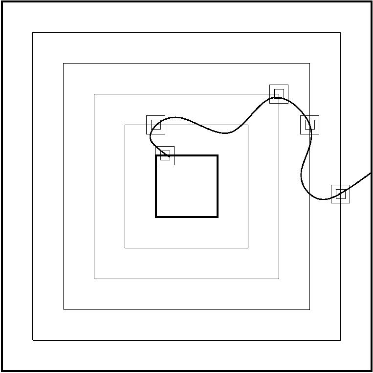
Figure 1: One way to define $y_{i}$ is as the closest vertex in $\mathbb{G}_{n-1}\cap\partial B(0,L_{n}+5L_{n-1}i)$ to the point of the first intersection of $\pi$ with $\partial B(0,L_{n}+5L_{n-1}i)$. Concentric boxes are not drawn to scale here: the innermost box is $B(0,L_{n})$, the outermost box is $B(0,2L_{n})$, and the intermediate boxes are $B(0,L_{n}+5L_{n-1}i)$, for $i\in\{1,\ldots,m_{0}\}$. The smallest and second smallest boxes along the path $\pi$ are $B(y_{i},L_{n-1})$ and $B(y_{i},2L_{n-1})$, respectively, for $i\in\{0,\ldots,m_{0}\}$.

By the definition of $m_{0}$ and $y_{i}$’s, all the boxes $B(y_{i},2L_{n-1})$ are disjoint and contained in $[-2L_{n},2L_{n})^{d}$, and the path $\pi$ connects $B(y_{i},L_{n-1})$ to the boundary of $B(y_{i},2L_{n-1})$, i.e., the event $\overline{H}^{*}(y_{i},L_{n-1},2L_{n-1})$ occurs for all $i\in\{0,\ldots,m_{0}\}$. We will show that

$$\begin{split}\text{there exists $j$ such that all the $4^{d}$ vertices in $\mathbb{G}_{n-1}\cap(y_{j}+[-2L_{n-1},2L_{n-1})^{d})$ are $(n-1)$-good,}\end{split}$$ (5.5)

which will contradict our assumption that (5.4) holds for $n-1$.

Since all the vertices in $\mathbb{G}_{n}\cap[-2L_{n},2L_{n})^{d}$ are $n$-good by assumption, it follows from (5.3) that

$$\begin{split}\text{there exist }&\text{$z_{1},\ldots,z_{3\cdot 4^{d}}\in[-2L_{n},2L_{n})^{d}$ such that}\\ &\text{all the vertices in $(\mathbb{G}_{n-1}\cap[-2L_{n},2L_{n})^{d})\setminus\cup_{i=1}^{3\cdot 4^{d}}B(z_{i},L_{n}/l(d))$ are $(n-1)$-good.}\end{split}$$ (5.6)

Note that each of the balls $B(z,2L_{n}/l(d))$ contains at most $(4(L_{n}/l(d))+1)/(5L_{n-1})\leq l_{0}/l(d)$ different $y_{i}$’s. Therefore, the union of the balls $\cup_{i=1}^{3\cdot 4^{d}}B(z_{i},2L_{n}/l(d))$ (with $z_{i}$’s defined in (5.6)) contains at most $3\cdot 4^{d}\cdot l_{0}/l(d)$ different $y_{i}$’s, which is strictly smaller than $m_{0}$ by the choice of $l(d)$ in (3.3). We conclude that there exists $j\in\{0,\ldots,m_{0}\}$ such that

$$y_{j}\notin\cup_{i=1}^{3\cdot 4^{d}}B(z_{i},2L_{n}/l(d)).\$$

We assume that $l_{0}$ is chosen large enough so that $L_{n}/l(d)>2L_{n-1}$, i.e., $l_{0}>2l(d)$. With this choice of $l_{0}$,

$$B(y_{j},2L_{n-1})\subseteq[-2L_{n},2L_{n})^{d}\setminus\cup_{i=1}^{3\cdot 4^{d}}B(z_{i},L_{n}/l(d)).\$$ (5.7)

Therefore, (5.5) follows from (5.6) and (5.7), which is in contradiction with the assumption that (5.4) holds for $n-1$. This implies that (5.4) holds for all $n\geq 0$. The proof of Lemma 6 is completed. ∎

6 Proofs of Theorem 1 and Theorem 2

In this section, we derive Theorems 1 and 2 from Lemmas 5 and 6.

Proof of Theorem 1.

The two results of Theorem 1 can be proved similarly (note that the results of Sections 3-5 can be trivially adapted to site percolation on $\mathcal{I}^{u}$), therefore we only provide a proof for the case of bond percolation on ${\widetilde{\mathcal{I}}}^{u}$.

Choose $L_{0}$ and $p<1$ such that Lemma 6 holds. Remember the definitions of a bad vertex and the event $\overline{H}^{*}(0,N)$ from Section 5. Let $M$ be a positive integer. Note that the probability that there exists a $*$-circuit of bad vertices in $\mathbb{G}_{0}\cap({\mathbb{Z}}^{2}\times\{0\}^{d-2})$ around $[0,L_{0}M)^{2}\times\{0\}^{d-2}$ is at most

$$\sum_{N=M}^{\infty}\mathbb{P}[\overline{H}^{*}(0,L_{0}N)]\leq C\sum_{N=M}^{\infty}e^{-N^{c}}\leq 1/2,\$$

for large enough $M$. If there is no such circuit, then, by planar duality (see, e.g., [10, Chapter 3.1]), there is a nearest-neighbor path $\pi=(x_{0},x_{1},\ldots)$ of good vertices in $\mathbb{G}_{0}\cap({\mathbb{Z}}^{2}\times\{0\}^{d-2})$ that connects $[0,L_{0}M)^{2}\times\{0\}^{d-2}$ to infinity. Namely, for all $i$, $x_{i}\in\mathbb{G}_{0}\cap({\mathbb{Z}}^{2}\times\{0\}^{d-2})$, $|x_{i}-x_{i+1}|_{1}=L_{0}$, $x_{i}$ is good, $x_{0}\in[0,L_{0}M)^{2}\times\{0\}^{d-2}$, and $|x_{n}|_{\infty}\to\infty$ as $n\to\infty$. It follows from Lemma 5 that the graph $\{{\widetilde{e}}~{}:~{}{\widetilde{e}}\in x+[0,2L_{0})^{d}~{}\mbox{for some }x\in\pi\}\subset{\mathbb{Z}}^{2}\times[0,2L_{0})^{d-2}$ contains an infinite connected component of ${\widetilde{\mathcal{I}}}^{u}\cap{\widetilde{\mathcal{B}}}^{p}$. Therefore, the probability that an infinite nearest-neighbor path in ${\widetilde{\mathcal{I}}}^{u}\cap{\widetilde{\mathcal{B}}}^{p}$ visits $[0,L_{0}M+2L_{0})^{2}\times[0,2L_{0})^{d-2}$ is at least $1/2$. By the ergodicity of ${\widetilde{\mathcal{I}}}^{u}\cap{\widetilde{\mathcal{B}}}^{p}$, an infinite nearest-neighbor path in $({\widetilde{\mathcal{I}}}^{u}\cap{\widetilde{\mathcal{B}}}^{p})\cap({\mathbb{Z}}^{2}\times[0,2L_{0})^{d-2})$ exists with probability $1$. ∎

Proof of Theorem 2.

We will use the main result of [13] that for an infinite graph $G=(V,E)$ and i.i.d. positive random variables $R_{\widetilde{e}}$, ${\widetilde{e}}\in E$, the following statements are equivalent: (a) almost surely, the electric network $\{R_{\widetilde{e}}~{}:~{}{\widetilde{e}}\in E\}$ is transient, and (b) for some $p<1$, independent bond percolation on $G$ with parameter $p$ contains with positive probability a cluster on which simple random walk is transient. (In the proof, we will only use the easy implication, namely, that (b) implies (a).)

Therefore, in order to prove Theorem 2, it suffices to show that for some $p<1$, with positive probability, the graph ${\widetilde{\mathcal{I}}}^{u}\cap{\widetilde{\mathcal{B}}}^{p}$ contains a transient subgraph. The proof of this fact is similar to the proof of Theorem 1 in [17], so we only give a sketch here.

Let $d\geq 3$ and $u>0$. Denote by $S^{d}$ the $d$-dimensional Euclidean unit sphere. We will show that, for any $\varepsilon\in(0,1)$, there exists an event $\mathcal{H}$ of probability $1$ such that if $\mathcal{H}$ occurs, then

$$\begin{split}\text{the graph ${\widetilde{\mathcal{I}}}^{u}\cap{\widetilde{\mathcal{B}}}^{p}$}&\text{ contains an infinite connected subgraph}\\ &\text{which, for each $v\in S^{d}$, contains an infinite path in the set $\cup_{n=1}^{\infty}B(nv,2n^{\varepsilon})$.}\end{split}$$ (6.1)

(The set $\bigcup_{n=1}^{\infty}B(nv,2n^{\varepsilon})$ is roughly shaped like a paraboloid with an axis parallel to $v$.) After that, one can proceed, as in Section 3 of [17], to show that this infinite connected subgraph of ${\widetilde{\mathcal{I}}}^{u}\cap{\widetilde{\mathcal{B}}}^{p}$ is transient.

Remember the definitions of the bad vertex and the event $\overline{H}^{*}(x,N)$ from Section 5. Let $L_{0}$ and $p<1$ satisfy Lemma 6. By (5.1) and the Borel-Cantelli lemma, for any $\varepsilon\in(0,1)$, the following event $\mathcal{H}$ has probability $1$: there exists a (random) $m$ such that for all $x\in\mathbb{G}_{0}$ with $|x|_{\infty}\geq mL_{0}$, the event $\overline{H}^{*}(x,|x|_{\infty}^{\varepsilon})$ does not occur. It remains to show that if the event $\mathcal{H}$ occurs, then (6.1) holds.

We will first prove that the event $\mathcal{H}$ implies that

(a) for each $v\in S^{d}$, there is a nearest-neighbor path $\pi_{v}$ of good vertices in $\mathbb{G}_{0}\cap\cup_{n=1}^{\infty}B(nv,n^{\varepsilon})$ that connects $B(0,mL_{0})$ to infinity, and

(b) all the paths $\pi_{v}$ are connected by nearest-neighbor paths of good vertices in $\mathbb{G}_{0}\cap B(0,2mL_{0})$.
Indeed, assume first that (a) fails, i.e., there exists $v\in S^{d}$ such that the set of vertices $y\in\mathbb{G}_{0}\cap\cup_{n=1}^{\infty}B(nv,n^{\varepsilon})$ connected to $B(0,mL_{0})$ by a nearest-neighbor path of good vertices in $\mathbb{G}_{0}\cap\cup_{n=1}^{\infty}B(nv,n^{\varepsilon})$ is finite. By [5, Lemma 2.1] or [27, Theorem 3], the boundary of this set contains a $*$-connected subset $\mathcal{S}$ of bad vertices in $\mathbb{G}_{0}\cap\cup_{n=1}^{\infty}B(nv,n^{\varepsilon})$ such that any nearest-neighbor path from $B(0,mL_{0})$ to infinity in $\mathbb{G}_{0}\cap\cup_{n=1}^{\infty}B(nv,n^{\varepsilon})$ intersects $\mathcal{S}$. In particular, there exists $x\in\mathbb{G}_{0}$ with $|x|_{\infty}\geq mL_{0}$, such that the event $\overline{H}^{*}(x,|x|_{\infty}^{\varepsilon})$ occurs; and, therefore, the event $\mathcal{H}$ does not occur.

Similarly, if (a) holds and (b) fails, then there exist at least two disjoint connected components of good vertices of diameter $\geq mL_{0}$ in $\mathbb{G}_{0}\cap(B(0,2mL_{0})\setminus B(0,mL_{0}-1))$ that intersect $B(0,mL_{0})$. Therefore, by [5, Lemma 2.1] or [27, Theorem 3], there exists $x\in\mathbb{G}_{0}$ with $|x|_{\infty}=mL_{0}$ such that the event $\overline{H}^{*}(x,mL_{0})$ occurs. This again implies that the event $\mathcal{H}$ does not occur.

It remains to notice that by (a), (b) and Lemma 5, the occurence of $\mathcal{H}$ implies (6.1). Indeed, Lemma 5 and (a) imply that there is an infinite path of ${\widetilde{\mathcal{I}}}^{u}\cap{\widetilde{\mathcal{B}}}^{p}$ in every set $\bigcup_{n=1}^{\infty}B(nv,2n^{\varepsilon})$, $v\in S^{d}$, and Lemma 5 and (b) imply that all these infinite paths are in the same connected subgraph of ${\widetilde{\mathcal{I}}}^{u}\cap{\widetilde{\mathcal{B}}}^{p}$.

Therefore, we have constructed the event $\mathcal{H}$ of probability $1$ which implies (6.1). In order to show that the infinite cluster in (6.1) is transient, we proceed identically to the proof of Theorem 1 in Section 3 of [17]. We omit further details. ∎

7 Proof of Theorem 3

In this section we prove Theorem 3. The first statement of Theorem 3 is proved in Section 7.1. In Section 7.2 we state Theorem 5, which implies the second statement of Theorem 3. The result of Theorem 5 is more general than the one of Theorem 3, since it also provides explicit upper and lower bounds on $u_{*}(\varepsilon)$, as $\varepsilon\to 0$. We prove Theorem 5 in Section 7.3.

7.1 Existence of phase transition

In this section we prove the first statement of Theorem 3. It follows from the next lemma.

Lemma 7.

For any $0<u<u^{\prime}$ and $\varepsilon\in(0,1/2)$, the set $\mathcal{V}^{u^{\prime},\varepsilon}$ is stochastically dominated by $\mathcal{V}^{u,\varepsilon}$. In particular, for any $u>u_{*}(\varepsilon)$, almost surely, the set $\mathcal{V}^{u,\varepsilon}$ does not contain an infinite connected component.

Proof.

Note that by the construction of $(\mathcal{I}^{u})_{u>0}$, on the same probability space in [22, (1.53)], the set $\mathcal{I}^{u}$ is stochastically dominated by $\mathcal{I}^{u^{\prime}}$ for $u<u^{\prime}$.

Let $\varepsilon\in(0,1/2)$. Let $\xi_{x}$, $x\in{\mathbb{Z}}^{d}$, be independent Bernoulli random variables with parameter $\varepsilon$, and $\eta_{x}$, $x\in{\mathbb{Z}}^{d}$, independent Bernoulli random variables with parameter $(1-2\varepsilon)/(1-\varepsilon)$, the two families are mutually independent, and also independent from the random interlacement $\mathcal{I}^{u}$. Let $\varphi_{x}=\max(\xi_{x},\eta_{x}\mathds{1}(x\in\mathcal{I}^{u}))$. It is easy to see that given $\mathcal{I}^{u}$, the $\varphi_{x}$ are independent, and the probability that $\varphi_{x}=1$ equals $\varepsilon$ for $x\in\mathcal{V}^{u}$, and $(1-\varepsilon)$ for $x\in\mathcal{I}^{u}$. Therefore, the set of vertices $\{x\in{\mathbb{Z}}^{d}~{}:~{}\varphi_{x}=1\}$ has the same distribution as $\mathcal{I}^{u,\varepsilon}$. Since, for $u<u^{\prime}$, $\mathcal{I}^{u}$ is stochastically dominated by $\mathcal{I}^{u^{\prime}}$, we deduce that $\mathcal{I}^{u,\varepsilon}$ is stochastically dominated by $\mathcal{I}^{u^{\prime},\varepsilon}$, and, therefore, $\mathcal{V}^{u^{\prime},\varepsilon}$ is stochastically dominated by $\mathcal{V}^{u,\varepsilon}$. ∎

7.2 Phase transition is non-trivial

In this section we state that for small enough $\varepsilon>0$, $u_{*}(\varepsilon)\in(0,\infty)$ and give explicit upper and lower bounds on $u_{*}(\varepsilon)$, as $\varepsilon\to 0$. The main result of this section is Theorem 5, which will be proved in Section 7.3. In order to state the theorem, we need to define the critical thresholds $\overline{u}$ and $u_{**}$.

Remark 2.

The earlier version of this paper contained a different proof of the fact that $u_{*}(\varepsilon)\in(0,\infty)$. It was based on a new notion of the so-called strong supercriticality in slabs. That proof is available in the first version of this paper on the arXiv [18]. The proof we present here is significantly simpler and relies on recent local uniqueness results of [7].

Definition 7.1.

Let $d\geq 3$. Let $\overline{u}=\overline{u}(d)$ be the supremum over all $u^{\prime}$ such that for each $u$ smaller than $u^{\prime}$, there exist constants $c=c(d,u)>0$ and $C=C(d,u)<\infty$ such that for all $n\geq 1$, we have

$$\mathbb{P}\left[B(0,n)\leftrightarrow\infty\mbox{ in }\mathcal{V}^{u}\right]\geq 1-Ce^{-n^{c}},\$$ (7.1)

and

$$\mathbb{P}\left[\begin{array}[]{c}\text{any two connected subsets of $\mathcal{V}^{u}\cap B(0,n)$ with}\\ \text{diameter $\geq n/10$ are connected in $\mathcal{V}^{u}\cap B(0,2n)$}\end{array}\right]\geq 1-Ce^{-n^{c}}.\$$ (7.2)

Note that Definition 7.1 implicitly implies that the right hand side of (7.1) must be positive for all $u<\overline{u}$ and large enough $n$. In particular, we conclude that $\overline{u}\leq u_{*}<\infty$. It was recently proved in [7, Theorem 1.1] (and, for $d\geq 5$, earlier in [25, (1.2) and (1.3)]) that

$$\overline{u}>0\mbox{ for all }d\geq 3.\$$ (7.3)

Let us also recall the definition of $u_{**}$ from [21, (0.6)] and [23, (0.10)]:

$$u_{**}=\inf\left\{u\geq 0\;:\;\liminf_{L\to\infty}\mathbb{P}\left[\begin{array}[]{c}\text{$B(0,L)$ is connected to the boundary of $B(0,2L)$}\\ \text{by a nearest-neighbor path in $\mathcal{V}^{u}$}\end{array}\right]=0\right\}.\$$ (7.4)

It follows from [19, 22, 23] that

$$u_{*}\leq u_{**}<\infty\mbox{ for all }d\geq 3.\$$

We prove the following theorem.

Theorem 5.

Let $d\geq 3$. We have

$$0<\overline{u}\leq\liminf_{\varepsilon\to 0}u_{*}(\varepsilon)\leq\limsup_{\varepsilon\to 0}u_{*}(\varepsilon)\leq u_{**}<\infty.\$$ (7.5)

Remark 3.

It would be interesting to understand whether the phase transition of $\mathcal{V}^{u}$ is actually stable with respect to small random noise. In other words, is it true that

$$\lim_{\varepsilon\to 0}u_{*}(\varepsilon)=u_{*}?$$ (7.6)

Based on (7.5), an affirmative answer to (7.6) will be obtained as soon as one proves that

$$\overline{u}=u_{*}=u_{**}.\$$ (7.7)

Note that the thresholds $\overline{u}$ and $u_{**}$ are defined purely in terms of $\mathcal{V}^{u}$, and not $\mathcal{V}^{u,\varepsilon}$. The statement (7.7) is about local connectivity properties of sub- and supercritical phases of $\mathcal{V}^{u}$. In the context of Bernoulli percolation, similar thresholds can be defined, and it is known that they coincide with the threshold for the existence of an infinite component (see, e.g., [10, (5.4) and (7.89)]), i.e., the analogue of (7.7) holds. The main challenge in proving (7.7) comes from the long-range dependence in $\mathcal{V}^{u}$ and the lack of the so-called BK-inequality (see, e.g., [10, (2.12)]), and hence it is interesting in its own.

7.3 Proof of Theorem 5

Recall the definition of $\mathcal{B}^{\varepsilon}$ from the beginning of Section 2. In order to prove (7.5), it suffices to show that

$$\forall\,u<\overline{u}\quad\exists\,\varepsilon_{0}(u)>0\quad\forall\,\varepsilon<\varepsilon_{0}(u)\,:\quad \mathbb{P}[0\stackrel{{\scriptstyle\mathcal{V}^{u}\setminus\mathcal{B}^{\varepsilon}}}{{\longleftrightarrow}}\infty]>0,\quad\mbox{and}$$ (7.8)

$$\forall\,u>u_{**}\quad\exists\,\varepsilon_{0}(u)>0\quad\forall\,\varepsilon<\varepsilon_{0}(u)\,:\quad \mathbb{P}[0\stackrel{{\scriptstyle\mathcal{V}^{u}\cup\mathcal{B}^{\varepsilon}}}{{\longleftrightarrow}}\infty]=0.\$$ (7.9)

The proofs of these statements are very similar to the proof of Theorem 1. Therefore, we only sketch the main ideas here.

We begin with the proof of (7.8). Let

$$\eta(u)=\mathbb{P}\left[0\leftrightarrow\infty\mbox{ in }\mathcal{V}^{u}\right].\$$ (7.10)

Note that $u_{*}=\inf\{u\geq 0~{}:~{}\eta(u)=0\}$. It follows from [24, Corollary 1.2] that

$$\eta(u) [0,u^{*})$$ is continuous on . (7.11)

Definition 7.2.

For $u>0$ and $k\geq 0$, let $\mathcal{V}^{u}_{k}$ be the subset of vertices of $\mathcal{V}^{u}$ which are in connected components of diameter $\geq k$ in $\mathcal{V}^{u}$.

By (7.10) and Definition 7.2, $\mathbb{P}[0\in\mathcal{V}^{u}_{k}]\geq\eta(u)$ and $\mathbb{P}[0\in\mathcal{V}^{u}_{k}]\to\eta(u)$ as $k\to\infty$. Therefore, by an appropriate ergodic theorem (see, e.g., [9, Theorem VIII.6.9] and [22, Theorem 2.1]), we get

$$\lim_{L\to\infty}\frac{1}{L^{d}}\sum_{x\in[0,L)^{d}}\mathds{1}\left(\,x\in\mathcal{V}^{u}_{L}\,\right)\;\stackrel{{\scriptstyle\mathbb{P}\text{-a.s.}}}{{=}}\;\lim_{L\to\infty}\frac{1}{L^{d}}\sum_{x\in[0,L)^{d}}\mathds{1}\left(\,x\leftrightarrow\infty\mbox{ in }\mathcal{V}^{u}\,\right)\;\stackrel{{\scriptstyle\mathbb{P}\text{-a.s.}}}{{=}}\;\eta(u).\$$ (7.12)

Definition 7.3.

Let $u<\overline{u}$ and $L_{0}\geq 1$. We call $x\in\mathbb{G}_{0}$ a good vertex if the following conditions are satisfied:

• for all $e\in\{0,1\}^{d}$, the graph $\mathcal{V}^{u}_{L_{0}}\cap(x+eL_{0}+[0,L_{0})^{d})$ contains a connected component with at least $\frac{3}{4}\eta(u)L_{0}^{d}$ vertices, and all these $2^{d}$ components are connected in $\mathcal{V}^{u}\cap(x+[0,2L_{0})^{d})$,

• for all $e\in\{0,1\}^{d}$, $|\mathcal{V}^{u}_{L_{0}}\cap(x+eL_{0}+[0,L_{0})^{d})|\leq\frac{5}{4}\eta(u)L_{0}^{d}$,

• $(x+[0,2L_{0})^{d})\cap\mathcal{B}^{\varepsilon}=\emptyset$.

Otherwise we call $x$ a bad vertex. Note that the event $\{\text{$x$ is good}\}$ is measurable with respect to the $\sigma$-algebra generated by $\{\mathds{1}(y\in\mathcal{V}^{u})~{}:~{}y\in x+[-L_{0},3L_{0})^{d}\}$ and $\{\mathds{1}(z\in\mathcal{B}^{\varepsilon})~{}:~{}z\in x+[0,2L_{0})^{d}\}$.

Definition 7.3 is similar to the definition of a good vertex in Section 5, except that now we are dealing with $\mathcal{V}^{u}_{L_{0}}$, rather than with ${\widetilde{\mathcal{I}}}^{u}$. In particular, the event $\{\text{$x$ is good}\}$ pertains to the occupancy of the vertices of ${\mathbb{Z}}^{d}$ rather than the edges. The event in (i) corresponds to the event $E^{u}_{x}({\widetilde{\mathcal{I}}}^{u})$, the event in (ii) corresponds to the event $F^{u}_{x}({\widetilde{\mathcal{I}}}^{u})$, and the event in (iii) corresponds to the complement of the event $\overline{D}_{x}({\widetilde{\mathcal{B}}}^{p})$. The role of the continuous function $m(u)$ in Definitions 4.1 and 4.2 is played by $\eta(u)$ (see (7.11) and compare (7.12) to (4.1)). The role of Lemma 1 is played by the following lemma.

Lemma 8.

Let $d\geq 3$, $0<u<\overline{u}$, and $\varepsilon>0$. There exist constants $c=c(d,u,\varepsilon)>0$ and $C=C(d,u,\varepsilon)<\infty$ such that for all $R\geq 1$,

$$\mathbb{P}\left[\bigcap_{x,y\in\mathcal{V}^{u}_{\varepsilon R}\cap[0,R)^{d}}\left\{x\leftrightarrow y\quad\mbox{in}\quad\mathcal{V}^{u}\cap[-\varepsilon R,(1+\varepsilon)R)^{d}\right\}\right]\geq 1-Ce^{-R^{c}}.\$$ (7.13)

Proof of Lemma 8.

It suffices to consider $R\geq 1$ such that $\varepsilon R\geq 10$. Let $k=\lfloor\varepsilon R/10\rfloor$. For $z\in[0,R)^{d}$, let $\mathcal{A}_{z}$ be the event that

• $B(z,k)$ is connected to the boundary of $B(z,4k)$ in $\mathcal{V}^{u}$, and

• every two nearest-neighbor paths from $B(z,2k)$ to the boundary of $B(z,3k)$ in $\mathcal{V}^{u}$ are in the same connected component of $\mathcal{V}^{u}\cap B(z,6k)$.

Let $\mathcal{A}=\cap_{z\in[0,R)^{d}}\mathcal{A}_{z}$. By (7.1) and (7.2), there exist constants $\widetilde{c}=\widetilde{c}(d,u,\varepsilon)>0$ and $\widetilde{C}=\widetilde{C}(d,u,\varepsilon)<\infty$, such that for all $R$, we have

$$\mathbb{P}\left[\mathcal{A}\right]\geq 1-\widetilde{C}e^{-R^{\widetilde{c}}}.\$$

Therefore, it suffices to show that

the event $$\mathcal{A}$$ implies the event in (7.13). (7.14)

Let $x,y\in\mathcal{V}^{u}_{\varepsilon R}\cap[0,R)^{d}$. Let $\mathcal{C}_{x}$ and $\mathcal{C}_{y}$ be the connected components of $x$ and $y$ in $\mathcal{V}^{u}\cap[-\varepsilon R,(1+\varepsilon)R)^{d}$. We will show that if $\mathcal{A}$ occurs then $\mathcal{C}_{x}=\mathcal{C}_{y}$. Note that by the choice of $x,y$ and $k$, $\mathcal{C}_{x}$ contains a path from $x$ to the boundary of $B(x,4k)$, and $\mathcal{C}_{y}$ contains a path from $y$ to the boundary of $B(y,4k)$.

Assume that $\mathcal{A}$ occurs. Take a nearest-neighbor path $\pi=(z_{1},\ldots,z_{t})$ in $[0,R)^{d}$ from $x$ to $y$. For each $1\leq i\leq t-1$, the occurrence of the events $\mathcal{A}_{z_{i}}$ and $\mathcal{A}_{z_{i+1}}$ implies that (a) there exist nearest-neighbor paths $\pi_{1}$ and $\pi_{2}$ in $\mathcal{V}^{u}$, $\pi_{1}$ from $B(z_{i},k)$ to the boundary of $B(z_{i},4k)$, and $\pi_{2}$ from $B(z_{i+1},k)$ to the boundary of $B(z_{i+1},4k)$, and (since both paths connect $B(z_{i},2k)$ to the boundary of $B(z_{i},3k)$) (b) any two such paths are connected in $\mathcal{V}^{u}\cap B(z_{i},6k)$. This implies that $\mathcal{C}_{x}$ and $\mathcal{C}_{y}$ must be connected in $\mathcal{V}^{u}\cap\cup_{i=1}^{t}B(z_{i},6k)\subseteq\mathcal{V}^{u}\cap[-\varepsilon R,(1+\varepsilon)R)^{d}$. This finishes the proof of (7.14) and of the lemma. ∎

Using (7.11), (7.12), and Lemma 8, we can proceed similarly to the proof of (5.1) (see also the proofs of Corollaries 2 and 3 and Lemma 4) to show that for any $0<u<\overline{u}$, there exist $L_{0}\geq 1$, $c>0$ and $C<\infty$ such that for all $N$ divisible by $L_{0}$, we have

$$\begin{split}\mathbb{P}\left[\begin{array}[]{c}\text{$0$ is connected to the boundary of $B(0,N)$}\\ \text{by a $*$-path of bad vertices in $\mathbb{G}_{0}$}\end{array}\right]\leq Ce^{-N^{c}}.\ \end{split}$$ (7.15)

We now use planar duality, similarly to the proof of Theorem 1, to show that (7.15) implies that for large enough $L_{0}$,

$$\mathbb{P}\left[\begin{array}[]{c}\text{$0$ is connected to infinity}\\ \text{by a nearest-neighbor path of good vertices in $\mathbb{G}_{0}$}\end{array}\right]>0.\$$ (7.16)

Similarly to Lemma 5, we observe that if there exists an infinite nearest-neighbor path $\pi=(x_{1},\ldots)$ of good vertices in $\mathbb{G}_{0}$, then the set $\cup_{i=1}^{\infty}\left(x_{i}+[0,2L_{0})^{d}\right)$ contains an infinite nearest-neighbor path of $\mathcal{V}^{u}\setminus\mathcal{B}^{\varepsilon}$. This, together with (7.16), implies (7.8).

We proceed with the proof of (7.9). Let $u>u_{**}$, $L_{0}\geq 1$, and $\varepsilon\in(0,1/L_{0}^{d+1})$. Recall that $\mathbb{G}_{0}=L_{0}{\mathbb{Z}}^{d}$. We call $x\in\mathbb{G}_{0}$ a bad vertex if either

(a) there exists a nearest-neighbor path in $\mathcal{V}^{u}$ from $B(x,L_{0})$ to the boundary of $B(x,2L_{0})$,
or

(b) $\mathcal{B}^{\varepsilon}\cap B(x,2L_{0})\neq\emptyset$.
With the above choice of $\varepsilon$, the probability of event in (b) goes to $0$ as $L_{0}\to\infty$.

It follows from the definition of $u_{**}$ and the choice of $\varepsilon$ (similarly to the proof of (5.1)) that for any $u>u_{**}$, there exist $L_{0}\geq 1$, $c>0$ and $C<\infty$ such that for all $N$ divisible by $L_{0}$, we have

$$\begin{split}\mathbb{P}\left[\text{$0$ is connected to the boundary of $B(0,N)$ by a $*$-path of bad vertices in $\mathbb{G}_{0}$}\right]\leq Ce^{-N^{c}}.\ \end{split}$$

In particular, for any $u>u_{**}$ and large enough $L_{0}$, almost surely, there is no infinite nearest-neighbor cluster of bad vertices in $\mathbb{G}_{0}$. Finally, note that if $\pi$ is an infinite path in $\mathcal{V}^{u}\cup\mathcal{B}^{\varepsilon}$ from the origin, then the origin is in an infinite nearest-neighbor path of bad vertices in $\mathbb{G}_{0}$. This implies (7.9). ∎

Acknowledgements.

We thank A.-S. Sznitman for pointing out a connection between our results and questions of robustness to noise, which led to results discussed in Section 7, and for a careful reading of the manuscript.

References

- [1] M. Campanino and L. Russo (1985) An upper bound on the critical percolation probability for the three-dimensional cubic lattice. Ann. Probab. 13(2), 478-491.
- [2] J.T. Chayes, L. Chayes, D.S. Fisher and T. Spencer (1986) Finite-size scaling and correlation lengths for disordered systems. Phys. Rev. Lett. 57(24), 2999-3002.
- [3] J.T. Chayes, L. Chayes, D.S. Fisher and T. Spencer (1989) Correlation length bounds for disordered Ising ferromagnets. Comm. Math. Phys. 120, 501-523.
- [4] J. Černý and S. Popov (2012) On the internal distance in the interlacement set. Electronic Journal of Probability 17, article 29.
- [5] J.-D. Deuschel and A. Pisztora (1996) Surface order large deviations for high-density percolation. Probability Theory and Related Fields 104, 467-482.
- [6] P. Doyle and E. Snell (1984) Random walks and electrical networks. Carus Math. Monographs 22, Math. Assoc. Amer., Washington, D.C.
- [7] A. Drewitz, B. Ráth and A. Sapozhnikov (2012) Local percolative properties of the vacant set of random interlacements with small intensity. arXiv:1206.6635.
- [8] A. Drewitz, B. Ráth and A. Sapozhnikov (2012) On chemical distances and shape theorems in percolation models with long-range correlations. arXiv:1212.2885.
- [9] N. Dunford and J.T. Schwartz (1958) Linear operators, Volume 1, Wiley-Interscience, New York.
- [10] G.R. Grimmett (1999) Percolation. Springer-Verlag, Berlin, second edition.
- [11] B.I. Halperin and A. Weinrib (1983) Critical phenomena in systems with long-range-correlated quenched disorder. Phys. Rev. B 27(1), 413-427
- [12] H. Lacoin and J. Tykesson (2012) On the easiest way to connect points in the random interlacements process. arXiv:1206.4216.
- [13] R. Pemantle and Y. Peres (1996) On which graphs are all random walks in random environments transient? Random Discrete Structures, IMA Volume 76, D. Aldous and R. Pemantle (Editors), Springer-Verlag.
- [14] E. Procaccia and E. Shellef (2012) On the range of a random walk in a torus and random interlacements. arXiv:1007.1401v2.
- [15] E.B. Procaccia and J. Tykesson (2011) Geometry of the random interlacement. Electronic Communications in Probability 16, 528-544
- [16] B. Ráth and A. Sapozhnikov (2012) Connectivity properties of random interlacement and intersection of random walks. ALEA 9, 67-83.
- [17] B. Ráth and A. Sapozhnikov (2011) On the transience of random interlacements. Electronic Communications in Probability 16, 379-391.
- [18] B. Ráth and A. Sapozhnikov (2011) The effect of small quenched noise on connectivity properties of random interlacements. arXiv:1109.5086v1.
- [19] V. Sidoravicius and A.-S. Sznitman (2009) Percolation for the Vacant Set of Random Interlacements. Comm. Pure Appl. Math. 62(6), 831-858.
- [20] A.-S. Sznitman (2009) Random walks on discrete cylinders and random interlacements. Probab. Theory Relat. Fields 145, 143-174.
- [21] A.-S. Sznitman (2009) Upper bound on the disconnection time of discrete cylinders and random interlacements. Annals of Probability 37(5), 1715-1746.
- [22] A.-S. Sznitman (2010) Vacant set of random interlacements and percolation. Ann. Math. 171, 2039-2087.
- [23] A.-S. Sznitman (2012) Decoupling inequalities and interlacement percolation on . Inventiones mathematicae 187(3), 645-706.
- [24] A. Teixeira (2009) On the uniqueness of the infinite cluster of the vacant set of random interlacements. Annals of Applied Probability 19(1), 454-466.
- [25] A. Teixeira (2011) On the size of a finite vacant cluster of random interlacements with small intensity. Probability Theory and Related Fields 150(3-4), 529-574.
- [26] A. Teixeira and D. Windisch (2011) On the fragmentation of a torus by random walk. Comm. Pure App. Probab. 64(12), 1599-1646.
- [27] Á. Tímár (2011) Boundary-connectivity via graph theory. To appear in Proc. Amer. Math. Soc.
- [28] A. Weinrib (1984) Long-range correlated percolation. Phys. Rev. B 29(1), 387–395.
- [29] D. Windisch (2008) Random walk on a discrete torus and random interlacements. Elect. Communic. in Probab. 13, 140-150.