Cross-correlating the Thermal Sunyaev-Zel’dovich Effect and the Distribution of Galaxy Clusters

Abstract

We present the analytical formulas, derived based on the halo model, to compute the cross-correlation between the thermal Sunyaev-Zel’dovich (SZ) effect and the distribution of galaxy clusters. By binning the clusters according to their redshifts and masses, this cross-correlation, the so-called stacked SZ signal, reveals the average SZ profile around the clusters. The stacked SZ signal is obtainable from a joint analysis of an arcminute-resolution cosmic microwave background (CMB) experiment and an overlapping optical survey, which allows for detection of the SZ signals for clusters whose masses are below the individual-cluster detection threshold. We derive the error covariance matrix for measuring the stacked SZ signal, and then forecast for its detection from ongoing and forthcoming combined CMB-optical surveys. We find that, over a wide range of mass and redshift, the stacked SZ signal can be detected with a significant signal to noise ratio (total $S/N\;\hbox to0.0pt{\lower 2.5pt\hbox{$\sim$}\hss}\raise 1.5pt\hbox{$>$}\;10$), whose value peaks for the clusters with intermediate masses and redshifts. Our calculation also shows that the stacking method allows for probing the clusters’ SZ profiles over a wide range of scales, even out to projected radii as large as the virial radius, thereby providing a promising way to study gas physics at the outskirts of galaxy clusters.

I Introduction

Galaxy clusters are the most massive, gravitationally bound objects in the universe, and therefore, their properties, e.g., the cluster abundance and its redshift evolution, are very sensitive to the underlying cosmology including the nature of dark energy Vikhlininetal:09 ; Rozoetal:10 . The Sunyaev-Zel’dovich (SZ) effect SZ72 offers a unique means of finding clusters out to high redshift due to its redshift independence (see Car02, , for a review). The wide-field, arcminute-resolution experiments of the cosmic microwave background (CMB) such as the Planck satellite PlanckSZ:11 , the Atacama Cosmology Telescope (ACT) Fowleretal:10 , and the South Pole Telescope (SPT) SPT:10 , have been drawing a great attention, because such CMB surveys enable us to construct a catalog of SZ clusters under a homogeneous selection function out to high redshifts beyond $z=1$. Such a cluster catalog can in turn be used to carry out the high-precision cosmological probes (Haimanetal:01, ; LimaHu:05, ; OguTak11, , also see references therein).

In the light of cluster cosmology, combining the SZ survey with a multi-color optical survey offers a great synergy, if the two cover the same region of the sky. First, the multi-color optical survey provides an estimate for the redshift of each SZ-discovered cluster from the photometric redshifts of its member galaxies. Otherwise the cluster’s redshift is unknown due to the redshift independence of the SZ signal. Second, from such an optical survey, we can construct a catalog of clusters by finding the concentration of galaxies in angular and photometric redshift space GladdersYee:00 ; Koesteretal:07 . Hence, by combining the SZ and optical surveys, we can obtain a more robust catalog of clusters. Third, from the joint experiment, we can explore the cluster mass-observable scaling relation by combining various observables including the measured SZ signal strength and the optical richness (i.e. the number of member galaxies). We can also include the weak lensing measurement on an individual cluster basis Okabeetal:10b ; Marroneetal:11 , where the lensing signal is available from the same optical data set, by exploring in detail the lensing shearing effects on background galaxy shapes due to the foreground cluster (see, e.g., Okabeetal:10, , for a weak lensing study of galaxy clusters). The use of a well-calibrated mass-observable relation is of critical importance to attain the high-precision of cluster cosmology LimaHu:05 ; DETF

By cross-correlating the SZ map with the distribution of optically selected clusters for a sufficiently large cluster sample, one can statistically measure the SZ signals of these clusters – the so-called stacked SZ signal. The stacking method enables us to measure the SZ signals for halos down to relatively low masses as well as up to large projected radii, which otherwise are very difficult to measure on an individual cluster basis, because the signals are too small. In particular, the stacking method allows a tomographic reconstruction of the SZ signal as a function of redshift pen2 ; shao1 , while the CMB signal itself is by nature two-dimensional, reflecting the information projected between the last scattering surface and the observer. The stacked SZ signals are useful for studies of the mean cluster mass-observable relation thanks to the statistically-boosted signal-to-noise ratios. Furthermore, the stacked SZ signals can be used to study the intracluster gas physics and to falsify and/or refine our theoretical understanding of galaxy clusters li2 ; Shawetal:10 ; Lau09 ; FanHai07 ; NagKV07 ; Bat10 .

The initial attempts to measure the stacked SZ signals have been recently reported, including those by combining the WMAP or Planck data with the SDSS maxBCG cluster catalog scott1 ; pl3 and the ACT data with the SDSS luminous red galaxies (LRGs) Handetal:11 , which preferentially reside in massive halos. Such measurements will be further significantly improved by combining the arcminute-resolution, high-sensitivity CMB surveys with overlapping wide-field, deep optical surveys, e.g., the SPT survey with the Dark Energy Survey (DES) DES , and the ACT with the Subaru Hyper Suprime-Cam (HSC) Survey Miyazakietal:06 ; OguTak11 .

Hence the purpose of this paper is to study the prospects of measuring the stacked SZ signals from ongoing and upcoming combined SZ and optical surveys. To make predictions for the stacked SZ profiles, we model the distribution of the hot gas contributing to the SZ effect KomSel02 as well as the distribution of galaxy clusters according to the halo model CooShe02 . Our formulas should be useful for future stacked SZ analysis. Following OguTak11 , we derive the covariances of the stacked SZ measurements for clusters binned by their redshifts and masses, which quantify the statistical uncertainties in the measurements.

The outline of the paper is as follows. In Sec. II, we present our derivation for the formulas to calculate the cross-correlation between the SZ effect and the distribution of galaxy clusters, and give the covariance matrix for its measurement. In Sec. III, we forecast the prospects of measuring the stacked SZ signals from several ongoing and upcoming surveys, and discuss our results. Finally, we conclude in Sec. IV. Throughout this paper, we adopt the best-fit flat $\Lambda$CDM model from WMAP 7-yr results WMAP7 with $\Omega_{m}=0.27$, $\Omega_{b}=0.045$, $h=0.71$, $\sigma_{8}=0.8$, $n_{s}=0.96$.

II Theoretical Calculation

In this section, following the method developed in OguTak11 and ColKai88 (also see KomKit99, ; SchBer91, ; PeacockSmith:00, ; Seljak:00, ; MaFry:00, ; Sco01, ; CooShe02, ; TakadaBridle:07, ), we use the halo model to calculate the cross-correlation between the SZ effect and the distribution of galaxy clusters, and give the covariance matrix for its measurement.

II.1 The SZ Effect and the SZ Power Spectrum

The thermal SZ effect introduces the following fractional distortion to the CMB temperature measured at frequency $\nu$ and in the angular direction of $\hat{n}$ (see e.g. SZ72, ; Rep95, ; Car02, ):

$$\frac{\Delta T}{T}(x,\hat{n})=f(x)y(\hat{n}),$$ (1)

where we have defined the dimensionless frequency $x\equiv h\nu/k_{B}T$, with $h$ the Planck constant, $k_{B}$ the Boltzmann constant, and the frequency dependence of the effect $f(x)$ is given by

$$f(x)=x\coth\left(\frac{x}{2}\right)-4,$$ (2)

where relativistic corrections (see e.g. RepII95, ; ChaLas97, ; SazSun98, ; Ito98, ) have been neglected. Note, in the Rayleigh-Jeans (RJ) limit, $f(x)\rightarrow-2$. The Compton $y$-parameter $y(\hat{n})$ is proportional to the electron pressure $P_{e}$ projected along the line of sight:

$$y(\hat{n})=\frac{\sigma_{T}}{m_{e}c^{2}}\int_{\hat{n}}P_{e}d\ell,$$ (3)

where $\sigma_{T}$ is the Thomson cross section, $m_{e}$ is the electron mass, and $c$ is the speed of light.

Using the halo model, $y(\hat{n})$ can be expressed as

$$y(\hat{n}) = \frac{\sigma_{T}}{m_{e}c^{2}}\int\frac{cdz}{H(z)}\frac{1}{(1+z)}\int dM_{h}\int d^{3}x_{h}$$

$$\times\sum_{i}\delta_{D}(M_{h}-M_{i})\delta_{D}^{3}(\vec{x}_{h}-\vec{x}_{i})P_{e}(|\vec{x}-\vec{x}_{h}|,M_{h},z_{h}),$$

where $H(z)$ is the Hubble expansion rate at redshift $z$; $\delta_{D}$ stands for the Dirac delta function; $M_{i}$ and $\vec{x}_{i}$ are the mass and center position of the $i$-th halo on the light cone, and the sum is done over all the haloes; $P_{e}(|\vec{x}-\vec{x}_{h}|,M_{h},z_{h})$ is the pressure at position $\vec{x}$ of the electrons in the dark matter halo with mass $M_{h}$, redshift $z_{h}$, and centered at $\vec{x}_{h}$. Note that the 3-dimensional position $\vec{x}$ is specified by $(\chi,\hat{n})$, where $\chi$ is the comoving radial distance corresponding to redshift $z$ on the light cone.

By using the flat-sky approximation and the Limber approximation Limber:54 , we obtain the SZ power spectrum ColKai88 ; KomKit99 :

$$C_{\ell}^{\rm yy}=C_{\ell}^{\rm yy,1h}+C_{\ell}^{\rm yy,2h},$$ (5)

with the one- and two-halo term contributions, $C_{\ell}^{\rm yy,1h}$ and $C_{\ell}^{\rm yy,2h}$, given by

$$C_{\ell}^{\rm yy,1h} = f(x)^{2}\int dz\frac{d^{2}V}{dzd\Omega}\int dM\frac{dn}{dM}(M,z)|\tilde{y}_{\ell}(M,z)|^{2},$$

$$C_{\ell}^{\rm yy,2h} = f(x)^{2}\int dz\frac{d^{2}V}{dzd\Omega}P_{m}^{L}\left(k=\frac{\ell}{\chi},z\right)W^{y}_{\ell}(z)^{2},$$ (6)

where $d^{2}V/dzd\Omega=c\chi^{2}/H$ is the comoving volume element, $dn/dM$ is the halo mass function, $\tilde{y}_{\ell}(M,z)$ is the 2D Fourier transform of the Compton $y$-parameter profile of a cluster with mass $M$ and at redshift $z$, and $P_{m}^{L}(k,z)$ is the linear matter power spectrum. The function $W^{y}_{\ell}(z)$ is defined as

$$W^{y}_{\ell}(z)\equiv\int dM\frac{dn}{dM}(M,z)b(M,z)\tilde{y}_{\ell}(M,z),$$ (7)

where $b(M,z)$ is the halo bias. As can be seen from Eq. (6), the SZ power spectrum arises from the contributions of halos over all the redshift range, and therefore contains only the projected information.

Below in our calculation, we would use the halo mass function from Jen01 , specifically their Eq. (B3), and the halo bias from SheTor99 ; HuKra03 . To calculate the linear matter power spectrum, we use the transfer function from EH99 . Our model for the intra-cluster gas is taken from KomSel02 , where the gas is assumed to be in hydrostatic equilibrium with the dark matter potential, have a constant polytropic equation of state, and trace the dark matter density with a constant amplitude offset in the outer parts of a cluster. We use the virial overdensity BryNor98 ; Kuh05 to define the cluster mass, and truncate the gas profile at three times the virial radius $r_{\rm vir}$. As implied from hydrodynamic simulations, the gas profile may extend beyond $r_{\rm vir}$ due to various nonlinear processes such as shock heating, feedback from star formation etc. BryNor98 ; Kravtsovetal:05 . Hence, it would be interesting to study the gas properties out to these large radii, which can be explored by using the stacking analysis (see below for further discussion).

II.2 The Distribution of Galaxy Clusters and Its Power Spectrum

Given a cluster survey, the galaxy clusters can be binned according to their observed redshift $z_{\rm obs}$ and estimated mass $M_{\rm obs}$. Given $P(z_{\rm obs}|M,z)$ and $P(M_{\rm obs}|M,z)$, i.e. the probability distribution functions (PDFs) of observing $z_{\rm obs}$ and $M_{\rm obs}$ for a cluster with true redshift $z$ and true mass $M$, the probability that the cluster is selected to the “$a$”-th redshift bin with $z_{\rm obs}\in[z^{a}_{\rm obs,min},z^{a}_{\rm obs,max}]$ and the “$b$”-th mass bin with $M_{\rm obs}\in[M^{b}_{\rm obs,min},M^{b}_{\rm obs,max}]$ can be calculated by

$$S_{ab}(M,z) = \int_{z_{\rm obs,min}^{a}}^{z_{\rm obs,max}^{a}}dz_{\rm obs}P(z_{\rm obs}|M,z)$$ (8)

$$\times\int_{M_{\rm obs,min}^{b}}^{M_{\rm obs,max}^{b}}dM_{\rm obs}P(M_{\rm obs}|M,z),$$

where $S_{ab}$ is called the selection function. In the ideal case that both $z$ and $M$ can be measured accurately, which we would assume in the following calculation for simplicity, the PDFs become delta functions, and $S_{ab}$ reduces to

$$S_{ab}(M,z) = \Theta(z-z^{a}_{\rm obs,min})\Theta(z^{a}_{\rm obs,max}-z)$$ (9)

$$\times\Theta(M-M^{b}_{\rm obs,min})\Theta(M^{b}_{\rm obs,max}-M),$$

where $\Theta$ stands for the Heaviside step function.

With the halo model formulation, the 2-dimensional angular number density of galaxy clusters in the “$(ab)$”-th bin can be calculated by

$$n_{ab}^{2D}(\hat{n}) = \int dz\frac{d^{2}V}{dzd\Omega}\int dMS_{ab}(M,z)$$ (10)

$$\times\sum_{i}\delta_{D}(M-M_{i})\delta_{D}^{3}(\vec{x}-\vec{x}_{i}),$$

where all symbols have the same meaning as before. Its ensemble average is given by

$$\bar{n}_{ab}^{2D}=\int dz\frac{d^{2}V}{dzd\Omega}\int dMS_{ab}(M,z)\frac{dn}{dM}(M,z),$$ (11)

where we have used $\left\langle\sum_{i}\delta_{D}(M-M_{i})\delta_{D}^{3}(\vec{x}-\vec{x}_{i})\right\rangle=dn/dM$ Sco01 .

With similar approximations as before, the power spectrum for the distribution of two cluster samples that are in the “$(ab)$”-th and “$(a^{\prime}b^{\prime})$”-th bins, respectively, can be calculated by

$$C_{\ell,(ab,a^{\prime}b^{\prime})}^{\rm hh}=\int dz\frac{d^{2}V}{dzd\Omega}P_{m}^{L}\left(k=\frac{\ell}{\chi},z\right)W^{h}_{ab}(z)W^{h}_{a^{\prime}b^{\prime}}(z),$$ (12)

where $W^{h}_{ab}(z)$ is defined as

$$W^{h}_{ab}(z)\equiv\frac{1}{\bar{n}^{2D}_{ab}}\int dM\frac{dn}{dM}(M,z)S_{ab}(M,z)b(M,z).$$ (13)

As long as the redshift of clusters can be measured accurately, as we assume in this paper, only the clusters in the same redshift bin would correlate with one another, so we have $C_{\ell,(ab,a^{\prime}b^{\prime})}^{\rm hh}=\delta_{aa^{\prime}}^{K}C_{\ell,(ab,ab^{\prime})}^{\rm hh}$, where $\delta^{K}_{aa^{\prime}}$ is the Kronecker delta function. Note in this case, $W^{h}_{ab}(z)=0$ if $z$ is outside the “$a$”-th redshift bin. Hence, with redshift information, the cluster power spectrum is free of projection effect.

II.3 The Cross-Correlation: the Stacked SZ Profile

With Eqs. (LABEL:eqn:y) and (10) in hand, we are now ready to calculate the cross-correlation between the SZ signal (to be explicit, $\Delta T^{\rm SZ}/T_{\rm CMB}$) and the cluster distribution. Again by adopting the flat-sky approximation and the Limber approximation, the cross power spectrum for the SZ signal and the distribution of galaxy clusters in the “($ab$)”-th bin can be calculated by (also see OguTak11, , for the method of derivation)

$$C_{\ell,(ab)}^{y{\rm h}}=C_{\ell,(ab)}^{y{\rm h,1h}}+C_{\ell,(ab)}^{y{\rm h,2h}},$$ (14)

where the one- and two-halo term contributions are given by

$$C_{\ell,(ab)}^{y{\rm h,1h}} = \frac{f(x)}{\bar{n}^{2D}_{ab}}\int dz\frac{d^{2}V}{dzd\Omega}\int dM\frac{dn}{dM}(M,z)$$ (15)

$$\times S_{ab}(M,z)\tilde{y}_{\ell}(M,z),$$

$$C_{\ell,(ab)}^{y{\rm h,2h}}=f(x)\int dz\frac{d^{2}V}{dzd\Omega}P_{m}^{L}\left(k=\frac{\ell}{\chi},z\right)W_{ab}^{h}(z)W^{y}_{\ell}(z).$$ (16)

This is the Fourier-transform of the so-called stacked SZ profile, which practically, can be obtained from observation by averaging the SZ maps around the cluster centers and then averaging over the orientation. Hence, the center of cluster should be known a priori, e.g., from the position of the brightest cluster galaxy in the case that the cluster catalog is constructed from an optical survey as we have had in mind. Offsets of the “cluster centers” would cause dilution of the stacked signal at small-angles (high-multipoles). Since the effect can be straightforwardly included by using the method developed in OguTak11 , we here ignore it for simplicity. We also notice that real clusters usually have aspherical shapes and substructures, which are not taken into account in our halo model calculation. A careful study of their effects on the stacked SZ profile would involve comparison with hydrodynamical simulations (see, e.g., Bat11 for their effects on the SZ power spectrum), which are beyond the scope of the current paper.

Comparing with Eq. (6), one can find that, since the selection function $S_{ab}(z)$ or $W^{\rm h}_{ab}(z)$ vanishes outside the redshift bin of the clusters taken for the cross-correlation, the cross-power spectrum contains only the SZ contributions from clusters in the redshift bin. Put another way, the cross-correlation method allows a tomographic reconstruction of the SZ signal as a function of redshift (also see shao1, ; pen2, , for similar discussions). When the redshift slice is sufficiently narrow, the cross-power spectrum is equivalent to the three-dimensional power spectrum through the correspondence of $k=\ell/\chi$, under the assumption of statistical isotropy.

Perhaps more intuitive is the Fourier-transformed counterpart of the cross-power spectrum, i.e., the stacked y-profile, defined as

$$\left\langle y\right\rangle_{(ab)}\!(\theta)\equiv\frac{1}{f(x)}\int\frac{\ell d\ell}{2\pi}J_{0}(\ell\theta)C_{\ell,(ab)}^{y{\rm h}},$$ (17)

where $J_{0}(\ell\theta)$ is the zeroth order Bessel function. The stacked y-profile gives the average y-profile around the clusters in the bin, which have similar redshift and similar mass, hence gives the average projected pressure profile: $\left\langle\int\!dl~{}P_{e}(r,l)\right\rangle\!(r_{\perp})=m_{e}c^{2}\left\langle y\right\rangle(\theta)/\sigma_{T}$, where $r_{\perp}=\chi(z)\theta/(1+z)$. Under the assumption of statistical isotropy, the average 3-dimensional pressure profile is considered to be spherically symmetric, and therefore can be recovered from the stacked y-profile through a deprojection process. This is analogous to the average mass profile of the clusters obtained from the stacked lensing measurement Johnstonetal:07 ; Okabeetal:10 .

II.4 Measurement Uncertainties: the Covariance Matrix

Given a survey, the stacked SZ signal can be measured by constructing an estimator from the observed fields. Uncertainties on the estimated values can be obtained from their covariance matrix. Similar to the covariance matrix for the stacked lensing power spectrum OguTak11  (also see Kno95, ; Sco99, ), the covariance matrix for the stacked SZ power spectrum is given by

$${\rm Cov}\left(C_{\ell,(ab)}^{y{\rm h}},C_{\ell^{\prime},(a^{\prime}b^{\prime})}^{y{\rm h}}\right) = \frac{\delta^{K}_{\ell\ell^{\prime}}}{f_{\rm sky}(2\ell+1)\Delta\ell}$$ (18)

$$\times\left[\hat{C}_{\ell}^{yy}\hat{C}_{\ell,(ab,a^{\prime}b^{\prime})}^{\rm hh}+\hat{C}_{\ell,(ab)}^{y{\rm h}}\hat{C}_{\ell,(a^{\prime}b^{\prime})}^{y{\rm h}}\right],$$

where $f_{\rm sky}=\Omega_{s}/4\pi$ is the fraction of the survey sky, with $\Omega_{s}$ the survey area, $\Delta\ell$ is the width of the $\ell$ band used to estimate the power spectrum, and $C_{\ell}$ with a hat symbol denotes the corresponding power spectrum for the observed fields, i.e. including noise contamination. Note, for simplicity, we have assumed the fields to be Gaussian in this calculation. See KomSel02 ; ZhangSheth:07 for discussions on the importance of non-Gaussian errors.

For a CMB experiment, the fluctuations in the temperature field that is actually observed have contributions from the primary CMB anisotropy, as well as from various secondary anisotropies and foregrounds such as the thermal SZ effect, the kinetic SZ effect, radio point sources, infrared point sources, diffuse Galactic foregrounds etc, in addition to the instrumental noise TegEis00 . Since the thermal SZ effect has a different frequency-dependence from the other components, by combining the data from multiple frequencies, the thermal SZ signal can be extracted (see e.g. CooHu00, ).

Here, for definiteness, we adopt the minimum-variance subtraction technique presented in CooHu00 to extract the SZ signal, and, for simplicity, we include only the instrumental noise. Therefore, the observed SZ power spectrum is given by

$$\hat{C}_{\ell}^{yy}=C_{\ell}^{yy}+\frac{1}{\sum_{c}w_{c}s_{c}^{2}B_{c\ell}^{2}},$$ (19)

where we use the subscript “$c$” to label the quantities for different frequency channels; $w=(\sigma_{T}\theta_{\rm FWHM}/T_{\rm CMB})^{-2}$, with $\sigma_{T}$ the rms of the instrumental noise per pixel, and $\theta_{\rm FWHM}$ the full width, half-maximum (FWHM) of the beam, which is assumed to be Gaussian; $B_{\ell}$ is the Fourier transform of the beam profile, and $B_{\ell}^{2}=\exp[-\ell(\ell+1)\theta_{\rm FWHM}^{2}/(8\ln{2})]$. Note we aim at extracting the SZ signal in the RJ limit, so the observation at each frequency has been rescaled by the ratio of frequency dependence: $s=-f(x)/2$. Specifications of the CMB experiments considered in this paper are given in Table 1. Since the instrumental noise is not correlated with the distribution of clusters, we have

$$\hat{C}_{\ell}^{y{\rm h}}=C_{\ell}^{y{\rm h}}.$$ (20)

Finally, we include a shot noise in the observed cluster power spectrum:

$$\hat{C}_{\ell,(ab,a^{\prime}b^{\prime})}^{\rm hh}=C_{\ell,(ab,a^{\prime}b^{\prime})}^{\rm hh}+\frac{1}{\bar{n}^{2D}_{ab}}\delta^{K}_{aa^{\prime}}\delta^{K}_{bb^{\prime}}.$$ (21)

Likewise, we can derive the covariance matrix for the stacked $y$-profile, $\left\langle y\right\rangle_{(ab)}\!(\theta_{i})$, which is estimated by Fourier transforming the stacked SZ power spectrum and then averaging over an annular area around $\theta_{i}$ (see e.g. TakadaJain:09, , for a similar derivation of the covariance for the correlation functions of the lensing field). The covariance between $\left\langle y\right\rangle_{(ab)}\!(\theta_{i})$ and $\left\langle y\right\rangle_{(a^{\prime}b^{\prime})}\!(\theta_{j})$ is found to be

$${\rm Cov}\left(\left\langle y\right\rangle_{(ab)}\!(\theta_{i}),\left\langle y\right\rangle_{(a^{\prime}b^{\prime})}\!(\theta_{j})\right) = \frac{1}{\Omega_{s}f(x)^{2}}\int\frac{\ell d\ell}{2\pi}\bar{J}_{0}(\ell\theta_{i})$$ (22)

$$\times\bar{J}_{0}(\ell\theta_{j})\left(\hat{C}_{\ell}^{yy}\hat{C}_{\ell,(ab,a^{\prime}b^{\prime})}^{\rm hh}+\hat{C}_{\ell,(ab)}^{y{\rm h}}\hat{C}_{\ell,(a^{\prime}b^{\prime})}^{y{\rm h}}\right),$$

where $\bar{J}_{0}(\ell\theta_{i})$ is the average of $J_{0}(\ell\theta)$ over the annulus around $\theta_{i}$. However, due to the exponential form of the noise term for $\hat{C}_{\ell}^{yy}$, Eq. (22) leads to divergent results. To resolve this apparent problem, we instead calculate the covariance for the stacked beam-smoothed SZ profile, which is actually a direct observable. To calculate the beam-smoothed $y$-profile, we only need to multiply the integrand of Eq. (17) by $B_{\ell}$ to account for the beam convolution, and to get the covariance, we only need to multiply that of Eq. (22) by $B_{\ell}^{2}$, which removes the exponential divergence. Note that the covariance given by Eq. (22) does not vanish when $\theta_{i}\neq\theta_{j}$, i.e. the $y$-profiles at different angular bins are correlated with one another even when the field is Gaussian.

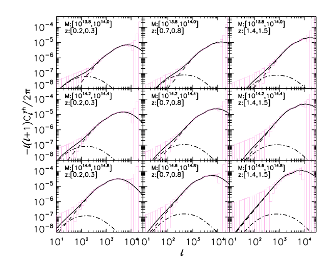
Figure 1: The cross power spectra of the SZ signal in the RJ band and the distribution of galaxy clusters in different redshift and mass bins. From left to right, the three columns are for clusters in the redshift bins of [0.2,0.3], [0.7,0.8] and [1.4,1.5], and from top to bottom, the rows are for clusters in the mass bins of $[10^{13.8},10^{14.0}]$, $[10^{14.2},10^{14.4}]$, $[10^{14.6},10^{14.8}]h^{-1}M_{\odot}$, respectively. The dashed and dot-dashed lines are the one- and two-halo term contributions, while the solid lines show the total. The boxes around each curve show $\pm 1\sigma$ statistical uncertainties in the power spectrum measurement expected for a 2500 deg² SPT-DES like survey, calculated as we describe in Sec. II.4.

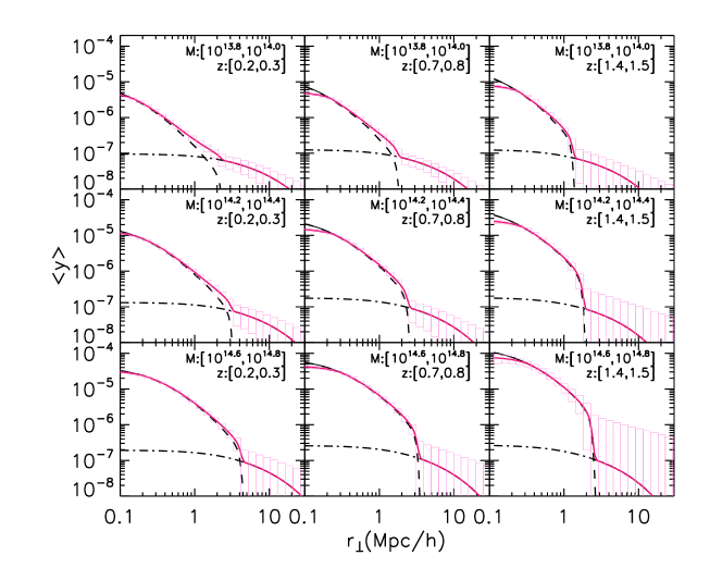
Figure 2: Similar to Figure 1, but here showing the stacked $y$-profiles for galaxy clusters in different redshift and mass bins, where the projected radius $r_{\perp}$ is converted from the angular separation $\theta$ by using the angular diameter distance for the mean redshift of the cluster bin. The error boxes are for the beam-smoothed stacked profiles for the SPT-DES like survey, where we use the beam for the 150GHz SPT channel. Note that the errors at different radii are correlated.

III Forecasts of the Stacked SZ Measurements

In this section, we estimate and discuss the detectability of the cross-correlation between the SZ map and the cluster distribution from ongoing and upcoming combined CMB and optical surveys.

III.1 Survey Parameters

Table 1: CMB Experimental Specifications

Experiment	$\Omega_{s}$(deg2)	$\nu$(GHz)	$\theta_{\rm FWHM}$(′)	$\sigma_{T}(\mu K)$
SPTwil01	2500	95	1.6	26.3
		150	1.1	16.4
		220	1.0	85
PlanckPlanck	41253	30	33	5.5
		44	24	7.4
		70	14	12.8
		100	10	6.8
		143	7.1	6.0
		217	5.0	13.1
		353	5.0	40.1
		545	5.0	400.6
		857	5.0	18257.5

Table 2: Optical Cluster Surveys

Survey	$\Omega_{s}$(deg2)	$z$-range
SDSS	7500	0.1-0.3
DES	5000	0.1-1.0
LSST	20000	0.1-1.4

Table 3: Combined SZ and Optical Cluster Surveys

Survey	$\Omega_{s}$(deg2)	$\ell_{\rm min}$	$\ell_{\rm max}$
SPT-DES	2500	7	$\sim 10000$
Planck-SDSS	7500	4	$\sim 3000$
Planck-LSST	20000	3	$\sim 3000$

To forecast the detectability of the stacked SZ signals from ongoing and upcoming surveys, we need to specify the survey parameters. In this paper, we consider the case that an optical survey, overlapped with a CMB survey, is used to construct a catalog of clusters. Such joint CMB and optical surveys that we are interested in include, e.g., DES and SPT, Subaru HSC and ACT, and SDSS or LSST and Planck.

As for the CMB surveys, specifications of each CMB experiment considered in this paper are given in Table 1. Table 2 gives the survey parameters for the optical surveys. Although an optical survey alone suffers from incompleteness of cluster finding, which may lead to a complicated selection function Koesteretal:07 ; Cohnetal:07 , we here assume that the optical survey can find all the clusters in the specified ranges of mass and redshift. Obviously this is too optimistic, and one should keep in mind that the following results give the best available case for the stacked SZ measurements. For a more realistic study, the selection function for a given survey needs to be properly taken into account. Table 3 gives the parameters for the joint CMB and optical surveys, including the overlapping area, the minimum and maximum multipoles probed.

III.2 Forecasts

In Figures 1 and 2, we show the stacked SZ power spectra, scaled to the RJ limit, and the stacked $y$-profiles for clusters in different redshift and mass bins. The dashed and dot-dashed curves in each panel are the one- and two-halo term contributions, respectively, while the solid curve represents the total. As can be seen, in Fourier space, the one-halo term dominates on small scales, while the two-halo term becomes more important on large scales, especially for the bins of clusters with lower masses and lower redshifts. Similar results hold in real space, except that the one-halo term is clearly truncated at about three times the virial radius of the most massive halo in each bin, as our gas profile is truncated at $r=3r_{\rm vir}$ (see § II.1). Note that we have converted the angular separation $\theta$ to the projected distance separation $r_{\perp}$ by using the (physical) angular diameter distance at the mean redshift of the bin. Thus, for a thin redshift slice, the stacking method probes the average projected pressure profile for the clusters stacked. In a statistically isotropic universe, the average 3D pressure profile is considered to be spherically symmetric, and therefore one can convert the projected pressure profile to obtain the 3D profile by using the Abel’s integral (see e.g. Eq. (1) in Johnstonetal:07, ).

The self-similar model predicts that the amplitude of the Compton $y$-parameter profile $y_{0}$ scales with the cluster’s virial density $\rho_{\rm vir}$ and virial mass $M_{\rm vir}$ as $y_{0}\propto\rho_{\rm vir}M_{\rm vir}$ (see the Appendix). Since $\rho_{\rm vir}$ increases with $z$, $y_{0}$ increases with $z$ as well, in addition to its increasing with $M_{\rm vir}$. These trends agree with what we see in Figures 1 and 2: the one-halo term for the cross correlation gets greater for cluster bins with higher $z$ and larger $M$, though the gas model we use is not exactly self-similar (broken by the dependence of the concentration parameter $c$ on $M_{\rm vir}$ and $z$). As the clusters become more massive and their redshifts get smaller, the angles they extend become larger, hence in real space, the one-halo term terminates at a larger angular scale, while in Fourier space, it peaks at a smaller $\ell$.

The error boxes around each curve in Figures 1 and 2 show the $1\sigma$ statistical uncertainties for measuring the stacked SZ signals at each multipole (radial) bin. These are expected for a 2500 deg² SPT-DES like survey. Note the error boxes at different radial bins for the stacked $y$-profile are correlated. These figures show that the stacking method can lead to a significant detection of the SZ signal over a wide range of multipoles or radii. In particular, it allows for exploration of the SZ signal at large radius, even around or beyond $r_{\rm vir}$, as can be seen from Figure 2. We find the variance of $C_{\ell}^{y{\rm h}}$ (Eq. 18) is mostly dominated by the term $\hat{C}^{\rm hh}_{\ell}\hat{C}^{yy}_{\ell}$. At $\ell\;\hbox to0.0pt{\lower 2.5pt\hbox{$\sim$}\hss}\raise 1.5pt\hbox{$>$}\;100$, it comes mainly from $\hat{C}^{yy}_{\ell}/\bar{n}^{2D}_{ab}$, and at even smaller scales such as $l\;\hbox to0.0pt{\lower 2.5pt\hbox{$\sim$}\hss}\raise 1.5pt\hbox{$>$}\;10^{4}$, instrumental noise dominates the error budget.

To be more quantitative, we calculate the cumulative signal-to-noise square $(S/N)^{2}$ for measuring the stacked SZ signals for the clusters binned by their redshifts and masses, which in Fourier space is an integration over a given range of multipoles, defined as

$$\left(\frac{S}{N}\right)^{2}=\sum_{\ell}C_{\ell,(ab)}^{y\rm{h}}{\rm Cov}^{-1}\left(C_{\ell,(ab)}^{y{\rm h}},C_{\ell,(ab)}^{y{\rm h}}\right)C_{\ell,(ab)}^{y{\rm h}}.$$ (23)

The $(S/N)^{2}$ is equivalent to the information content available from a Fisher matrix analysis TakBhu09 ; TegTay97 : given a template for the interested power spectrum, it gives the significance that the amplitude of the power spectrum is detected to be non-zero. We notice that the $(S/N)^{2}$ is proportional to the survey area $\Omega_{\rm s}$ (assuming a simple survey geometry).

In Figures 3-5, we plot the contours of the $S/N$ for the SPT-DES, Planck-SDSS, and Planck-LSST like surveys, respectively. Again note that we have assumed all the clusters in a given mass and redshift bin can be found from the survey, i.e. 100% completeness and efficiency of cluster finding. As we noticed before, the amplitude of the cross correlation increases when the clusters in the bin have larger masses or higher redshifts. At the same time, the number of clusters in the bin decreases with their masses, and also decreases with their redshifts, though it increases with the redshift at first. While the $S/N$ increases when the signal is higher, it decreases when the shot noise is larger. The result is that the $S/N$ peaks for some cluster bin at intermediate redshift and intermediate mass – the sweet spot, as can be seen from these three figures. From SPT to Planck, the resolution of the instruments gets worse, and the sweet spot shifts to lower redshift and higher mass, where the clusters extend larger angles such that their profiles can be better resolved. In particular, it would be interesting to notice that the arcminute-resolution CMB experiment such as SPT has the sweet spot at around $z\simeq 0.6$ and $M\simeq 2\times 10^{14}h^{-1}M_{\odot}$. From SDSS to LSST, the $S/N$ increases due to the larger survey area. Note $S/N\propto\sqrt{f_{\rm sky}}$, provided the probed $\ell$ ranges are similar.

Recently, the Planck team has shown their high significance detection of the SZ signals for the SDSS maxBCG clusters pl3 , down to the low mass systems. Their analysis is different from what we are doing in this paper. Instead of stacking the SZ maps around the center of each cluster, they derived the integrated SZ signal $Y_{500}$ for each cluster by employing a multi-frequency matched filter, and then calculated the weighted mean of the signal. The $S/N$ of their detection ranges roughly 4$\sim$15 for the cluster bins that are relatively narrower in mass and wider in redshift than ours. Despite the differences in analysis, their results are less optimal than ours. This may be because: the Planck results are from its first-year survey, so the instrumental noises are larger than their expected values, which are what we adopt in this paper; our results neglect the impurity and incompleteness of the maxBCG cluster catalog, hence tend to be optimal. Interestingly, we notice the $S/N$ of the Planck’s results also peaks at some intermediate mass $\sim 2\times 10^{14}h^{-1}M_{\odot}$ (corresponding to $N_{200}\sim 30$), which is smaller than what we find by roughly a factor of $2$.

Figure 3: Contours of the total signal-to-noise ratio (S/N) expected for measuring the cross-correlation between the SZ effect and the distribution of galaxy clusters assuming a SPT-DES like survey (see Eq. 23 for the definition of the S/N). The clusters are binned in redshift with $\Delta z=0.1$ and in mass with $\Delta\log(M_{\rm obs})=0.2$, respectively.

Figure 4: Similar to the previous plot, but for a Planck-SDSS like survey. Note here the contours are displayed out to much higher redshift regions than those available from the SDSS, which is z:[0.1,0.3].

Figure 5: Similar to Figure 3, but for a Planck-LSST like survey.

III.3 Residual Noise Contamination

Our estimation for the noise in the extracted SZ signal so far includes only the instrumental noise. This is optimistic, since there are various sources of contamination to the SZ effect, e.g. the point sources (both the Poisson distributed and clustered components) Lue10 ; Hal10 ; Fowleretal:10 ; PlanckCIB:11 , and the primary CMB fluctuations, which may leave some residual components even after the SZ signal has been maximally extracted. In this subsection, we consider two types of residual noise: those from the point sources and from the primary CMB, and see how the $S/N$ of the stacked SZ signal is degraded.

In the following, we give a simple estimate on the impact of these two types of residual noise on the measurement of the stacked SZ signal. The primary CMB fluctuations do not correlate with the distribution of clusters. Therefore, we assume the residual CMB does not contaminate the stacked SZ signal, but adds to its noise. We also assume the residual CMB has the same power spectrum as the primary CMB, for simplicity. As for the contamination from point sources, we need to consider two populations: radio sources such as galaxies hosting active galactic nuclei (AGNs), and infrared sources such as the dusty star-forming galaxies. Although radio sources tend to reside in clusters, their contamination to the SZ signal is unlikely to be significant (10% at most for low-$z$ clusters) Linetal:09 . On the other hand, infrared sources dominate the point source contamination to the SZ power, with both a Poisson-distributed and a clustered component. However, it is likely that the majority of contamination comes from galaxies at high redshifts such as $z\;\hbox to0.0pt{\lower 2.5pt\hbox{$\sim$}\hss}\raise 1.5pt\hbox{$>$}\;2$ PlanckCIB:11 , which do not correlate with the massive halos at $z\;\hbox to0.0pt{\lower 2.5pt\hbox{$\sim$}\hss}\raise 1.5pt\hbox{$<$}\;1.5$ as are considered in this paper. Hence we assume that the residuals from point sources do not contaminate $\hat{C}_{\ell}^{yh}$, but add to $\hat{C}_{\ell}^{yy}$. Specifically, we assume the residuals are Poisson distributed, and estimate their impact by simply doubling the instrumental noise.

The results of our calculation are shown in Figure 6. These are the $S/N$ contours for a SPT-DES like survey. In the upper right panel, we include the residual noise from the point sources, in the bottom left, we include that from the primary CMB, while in the bottom right, we include both. To easily see the effects of these residual noises, we show in the upper left panel our results before, i.e., with instrumental noise only. As is expected, the $S/N$ is reduced when either of the residual noises is included. According to our calculation for the residual power spectra, the primary CMB causes a larger reduction in the $S/N$ than the point sources, which perhaps indicates the necessity to remove the CMB. From Figure 1, we can also see, on scales where the primary CMB dominates ($\ell\;\hbox to0.0pt{\lower 2.5pt\hbox{$\sim$}\hss}\raise 1.5pt\hbox{$<$}\;3000$), there is non-negligible contribution to the total $S/N$. Finally, we find, even in the most pessimistic case we study, the $S/N$ for the detection of the stacked SZ signals for the less massive clusters fortunately remains substantial ($\;\hbox to0.0pt{\lower 2.5pt\hbox{$\sim$}\hss}\raise 1.5pt\hbox{$>$}\;20$).

Figure 6: Similar to Figure 3, but using different models for the noise in the SZ field. The upper-left panel is the same as Figure 3, shown here for comparison, which includes only the instrumental noise, the upper-right has the residual noise from point sources added in, the lower-left has that from the primary CMB added in, while the lower right has both (see text for the details).

IV Discussion

In this paper, we have developed the halo model based method to compute the stacked SZ profile of the galaxy clusters, measured by cross-correlating the SZ map and the clusters’ distribution, and the method to estimate the expected signal-to-noise ($S/N$) ratio for its detection from a given survey. Such stacked SZ signals can be obtained, e.g., by combining the arcminute-resolution CMB experiments with optical surveys such as the combination of the DES and SPT, or the Subaru HSC and ACT surveys.

Although the measured CMB signal is by nature two-dimensional, cross-correlating the CMB map with clusters of known redshifts allows for a tomographic reconstruction of the SZ signals as a function of redshift. In addition, simultaneous reconstruction of the SZ signals as a function of cluster mass is also allowed, if the clusters’ masses are also known. This would be very useful for carrying out the precision cosmology with cluster based experiments as well as studying the cluster astrophysics, in particular, its time evolution (see, e.g., FanHai07, ).

The stacked SZ signals will be very complementary to the stacked lensing signals Johnstonetal:07 ; Okabeetal:10 , if both methods study the same catalog of clusters. One of the crucial sources of systematic in cluster cosmology is from the mass-observable relation. To attain the precision of cluster cosmology, we need a well-calibrated mass-observable relation. Combining the stacked SZ and lensing signals for the same catalog of clusters will provide a powerful means of studying the mean relation between cluster mass and SZ signal as a function of redshift and mass (more precisely, the optical richness) from the observation. As we have shown, the stacking method can significantly reduce the statistical errors, and allows one to probe the SZ or lensing signals for the low mass clusters or to large angular scales (also see OguTak11, ). However, the scatters around the mean mass-observable relation still need to be understood, and detailed studies of the target cluster sample combining various observables will also be needed (e.g., see Marroneetal:11, , for such a multi-wavelength study).

Combining the stacked SZ and lensing signals will be powerful for studies of cluster physics as a function of cluster mass and redshift. Due to the statistical symmetry of the universe, the stacked pressure and mass profiles can be considered to be spherically symmetric in an average sense. Hence it would be of great interest to construct the cluster’s baryon fraction profile observationally, and then address at which radii the cosmic mean baryon fraction is reached. Since the intra-cluster gas may be blown off to outer radii by various feedback effects from e.g. AGN or supernova, which involve complicated astrophysical processes, such a model-independent method of studying the baryon fraction would be very useful (see Afshordietal:07, ; Umetsuetal:09, , for the related discussion).

The SZ signals from galaxy clusters would be smaller if there is a significant fraction of non-thermal pressure support from random gas motions, whose existence could help to explain the apparent conflict between the amplitude of the observed SZ power spectrum with theoretical prediction Shawetal:10 . Such non-thermal pressure support is expected to be more significant at the outskirts for given mass-scale halos Lau09 . Again the stacking method is very powerful for studying the SZ signals at such outer radii, which otherwise would be very difficult due to the faint signals.

Throughout this paper, we have been using the relatively simple analytical model from KomSel02 for the cluster pressure profile, given as a function of halo mass and redshift. It is known this model overestimates the measured SZ power spectrum amplitude (by about a factor of 2), which however would not alter our conclusion of a significant S/N for the stacked SZ measurement that is evident from Figure 3-5. However, a more careful study will be definitely needed, e.g., by using more realistic pressure profiles (see, e.g., Arn10, ), or hydrodynamic simulations, in order to realize the genuine power of the stacking method.

APPENDIX

In the self-similar model, the gas profiles of all the clusters are considered identical with appropriate choice of normalization factors that are the powers of the global quantities e.g. mass $M_{\rm vir}$, radius $r_{\rm vir}$. For example, the temperature profile can be expressed as $T(r)/T_{\rm vir}\propto f_{T}(r/r_{\rm vir})$, with $T_{\rm vir}\propto M_{\rm vir}/r_{\rm vir}$(from the virial theorem) and $f_{T}(r/r_{\rm vir})$ a universal function. Similarly, the pressure profile can be expressed as $P(r)/P_{\rm vir}\propto f_{P}(r/r_{\rm vir})$, with $P_{\rm vir}\propto\rho_{\rm vir}T_{\rm vir}$ and $f_{P}(r/r_{\rm vir})$ a universal function. Hence, the $y$-profile is given by

$$y(\theta) =\frac{\sigma_{T}}{m_{e}c^{2}}\int_{-\sqrt{r_{\rm vir}^{2}-r_{\perp}^{2}}}^{\sqrt{r_{\rm vir}^{2}-r_{\perp}^{2}}}P\left(\sqrt{\ell^{2}+r_{\perp}^{2}}\right)d\ell,$$ (24)

$$\propto P_{\rm vir}r_{\rm vir}f_{y}(r_{\perp}/r_{\rm vir}),$$

$$\propto\rho_{\rm vir}M_{\rm vir}f_{y}(\theta/\theta_{\rm vir}),$$

where $\theta_{\rm vir}=r_{\rm vir}/d_{A}$, with $d_{A}$ the angular diameter distance, and $f_{y}$ is a universal function. As can be seen, the amplitude of the self-similar $y$-profile is proportional to $\rho_{\rm vir}M_{\rm vir}$.