Quantum noise and mode nonorthogonality
in nonhermitian $\mathcal{PT}$-symmetric optical resonators

Abstract

$\mathcal{PT}$-symmetric optical resonators combine absorbing regions with active, amplifying regions. The latter are the source of radiation generated via spontaneous and stimulated emission, which embodies quantum noise and can result in lasing. We calculate the frequency-resolved output radiation intensity of such systems and relate it to a suitable measure of excess noise and mode nonorthogonality. The lineshape differs depending on whether the emission lines are isolated (as for weakly amplifying, almost hermitian systems) or overlapping (as for the almost degenerate resonances in the vicinity of exceptional points associated to spontaneous $\mathcal{PT}$-symmetry breaking). The calculations are carried out in the scattering input-output formalism, and are illustrated for a quasi one-dimensional resonator set-up. In our derivations we also allow for the more general case of a resonator in which the amplifying and absorbing regions are not related by symmetry.

I Introduction

Recent theoretical and experimental advances in optics R.El-Ganainy ; Z.H.Musslimani2 ; K.G.Makris ; S.Longhi ; C.E.Ruter ; A.Guo ; M.C.Zheng ; H.Ramezani ; A.A.Sukhorukov ; Z.Lin ; H.Schomerus ; S.Longhi2 ; Y.D.Chong have raised the prospect to realize nonhermitian systems with a real spectrum but nonorthogonal wave functions. These efforts are based on the concept of $\mathcal{PT}$ symmetry, originally formulated as a variant of quantum mechanics in which potentials can be complex C.M.Bender1 ; M.Znojil ; A.Mostafazadeh ; A.Mostafazadeh0 ; C.M.Bender3 ; F.G.Scholtz . In the optical context such potentials can be realized via absorbing and amplifying regions. In a $\mathcal{PT}$-symmetric situation, a discrete unitary operation (such as a reflection or inversion) maps the absorbing onto the amplifying parts, with matching absorption and amplification rates. On the level of classical optics, absorption and amplification are related by an antiunitary time-reversal operation. If the absorption and amplification rates are low enough, the spectrum of the composed system is real, but beyond a threshold pairs of complex conjugate eigenvalues appear C.M.Bender1 ; M.Znojil ; A.Mostafazadeh ; A.Mostafazadeh0 ; C.M.Bender3 ; F.G.Scholtz ; S.Klaiman ; S.Bittner . This transition (known as spontaneous $\mathcal{PT}$-symmetry breaking) can be exploited to realize a number of exotic optical effects, such as unidirectional transmission K.G.Makris ; H.Ramezani ; Z.Lin , absorption-enhanced transmission A.Guo , power oscillations K.G.Makris ; C.E.Ruter , nonlinear switching A.A.Sukhorukov , and coexistence of lasing and perfect absorption S.Longhi2 ; Y.D.Chong . At the transition point, eigenvalues coalesce, resulting in an exceptional point where the two eigenmodes become degenerate not only in frequency, but also share the same wave function T.Kato ; W.D.Heiss ; C.Dembowski ; M.V.Berry2 . This singular scenario receives considerable attention also for optical systems without $\mathcal{PT}$ symmetry S.Y.Lee ; J.Wiersig ; J.-W.Ryu ; B.Dietz2 ; L.Ge ; M.Liertzer .

In this paper, we investigate how the unavoidable consequences of leakage, instability, and quantum noise affect the characteristics of realistic $\mathcal{PT}$-symmetric resonators. In combination, we find that these effects offer a window to directly access the signatures of nonhermiticity. In particular, they allow to detect mode nonorthogonality, which discriminates these systems from ordinary hermitian systems that possess a real spectrum but feature mutually orthogonal eigenmodes.

In realistic devices, additional losses arise due to leakage, as radiation needs to be coupled out of the system. Even though these losses break exact $\mathcal{PT}$-symmetry, signatures of the associated peculiar spectral characteristics are still present in the complex resonance frequencies of the open system. The coalescence of eigenvalues at the spontaneous $\mathcal{PT}$-symmetry breaking transition then translates to situations where two resonance frequencies approach each other very closely in the complex plane.

In actively amplifying optical systems, the appearance of real eigenfrequencies indicates an instability, the onset of lasing. The consequences for $\mathcal{PT}$-symmetric systems have been explored only since very recently. In these systems, the lasing threshold is either reached in the limit of the closed system (if the spectrum in this limit is real) H.Schomerus , or at finite leakiness (if $\mathcal{PT}$ symmetry in the closed system is spontaneously broken, i.e., beyond an exceptional point) S.Longhi2 ; Y.D.Chong . In both cases, the system is in practice stabilized by saturation in the amplifying parts, thereby assuring that the output intensity remains finite. This saturation provides a physical mechanism that breaks the balance of amplification and absorption required for $\mathcal{PT}$ symmetry.

An ordinary laser emits coherent radiation with a narrow emission line that can be well approximated by a Lorentzian. According to general laser theory A.E.SiegmanBook ; A.L.Schawlow , the width $\Delta\omega$ of the Lorentzian arises due to noise, of which a certain amount, quantum noise, is an unavoidable consequence of the quantum nature of microscopic emission events. Investigations on purely amplifying (not $\mathcal{PT}$-symmetric) systems established a direct link of nonhermiticity and an enhanced line broadening (known as excess noise), which are both captured by a measure of mode nonorthogonality, the Petermann factor $K$ K.Petermann ; A.E.Siegman ; P.Goldberg ; G.H.C.New ; M.Patra ; H.Schomerus1 . At an exceptional point, $K$ diverges because of the coalescence of resonance wavefunctions T.Kato ; W.D.Heiss ; C.Dembowski ; M.V.Berry2 . $\mathcal{PT}$-symmetric systems offer an ideal venue where the consequences for the radiated intensity in this singular case can be explored. More generally, one should expect for such systems that the excess noise provides a probe of the level of nonhermiticity also away from an exceptional point.

The preceding observations capture our principal motivation for this work. It is the purpose of this paper to formulate a theory of the quantum noise and radiation of leaky $\mathcal{PT}$-symmetric optical systems in the full range of situations far below, near, and beyond the reconfiguration of the spectrum at an exceptional point, up to the point where the lasing threshold is reached. This requires a quantum optical treatment, which we base on the scattering input-output formalism M.J.Collett ; T.Gruner ; C.W.J.Beenakker , as previously applied to purely amplifying systems M.Patra ; H.Schomerus1 . Taking the absorbing parts of the system into account, we establish general relations for the output intensity as for the previously studied case of a homogeneously amplifying resonator, but find that this involves a nontrivial combination of aspects from mode nonorthogonality and excess noise. As one approaches an exceptional point, the partial intensities of the two near-degenerate resonances still diverge, but the combined amplitude remains finite, which signals a change in the lineshape from a Lorentzian to a squared Lorentzian (as also observed at exceptional points in passive scattering theory E.Hernandez ; N.J.Kylstra ; A.I.Magunov ).

We illustrate these general results on quantum noise for a specific quasi one-dimensional $\mathcal{PT}$-symmetric resonator, which displays the generic spectral properties of previously studied resonators M.Znojil ; Y.D.Chong and offers additional control via a variable leakage to the exterior. This application extends the investigation in Ref. H.Schomerus , which used the input-output formalism to study a ${\mathcal{P}T}$-symmetric resonator with well isolated resonances and did not address the relation to mode nonorthogonality. Throughout our derivations, we also present general expressions that apply to systems with amplifying and absorbing regions, even when these are not related by $\mathcal{PT}$ symmetry (as recently investigated, e.g., in Refs. L.Ge ; M.Liertzer ; Y.D.Chong0 ; J.Andreasen ).

This work is organized as follows. Section II reviews the spectral features of closed and open $\mathcal{PT}$-symmetric systems, as well as the signatures of excess quantum noise for conventional, amplifying resonators, with the discussion based in both cases on the common framework of (first- and second-quantized) scattering theory. In Section III we adapt the scattering input-output formalism to resonators with absorbing parts and derive general expressions for the output radiation intensity. In the central Section IV, we analyze this radiation near resonance and establish the link to mode nonorthogonality. Section V sees our general results applied to a specific $\mathcal{PT}$-symmetric resonator set-up. We first study the classical wave problem and determine the resonance frequencies and exceptional points. We then analyze the output radiation in the vicinity of these frequencies and verify the sensitivity to the nonorthogonality of modes, as well as the emergence of a squared Lorentzian at the exceptional points. Section VI contains our conclusions.

II Background and open issues

In this section we briefly review the (‘first-quantized’, classical-wave) scattering approach to the determination of eigenfrequencies and resonances in closed and open nonhermitian $\mathcal{PT}$-symmetric systems, as well as the application of the (‘second-quantized’, quantum-optical) scattering input-output formalism to the problem of excess noise in purely amplifying systems. Sections III and IV then extend the latter to partially absorbing systems, including those with $\mathcal{PT}$ symmetry. Throughout, we identify $\omega$ with the energy of photons (effectively setting $\hbar\equiv 1$).

II.1 Scattering quantization and spectral properties of $\mathcal{PT}$-symmetric systems

While scattering appears most naturally in the context of transport through open systems, the scattering framework can also serve as a convenient technique to determine spectral properties, such as the resonance eigenfrequencies of these systems, or even the bound-state spectrum of closed systems E.Doron ; E.B.Bogomolny . In scattering theory the eigenfrequencies are determined efficiently using a small number of basis functions, which are the on-shell (fixed energy or frequency) solutions in various, artificially separated (and therefore open) parts of the system, which then are coupled together using their scattering matrices. The quantization condition follows from the consistency requirement of the matching conditions. In the present work, the use of scattering theory is further motivated by the fact that it also can serve as a framework for introducing quantum noise. Indeed, we will find that the steps in the derivation of the quantization condition (given here) and in the implementation of quantum noise in composed systems (given in Sec. III) closely resemble each other. In this first part of background material, we therefore review the general ideas of spectral analysis in scattering theory, and also describe the consequences for systems with $\mathcal{PT}$ symmetry H.Schomerus ; Y.D.Chong (for other aspects of $\mathcal{PT}$-symmetric scattering theory see Refs. F.Cannata ; M.V.Berry3 ; H.F.Jones2 ; H.Schomerus3 ; H.Hernandez-Coronado ; K.Abhinav ).

II.1.1 Scattering matrix

We start with the definition of the relevant scattering matrix. Consider a classical wave equation, e.g., the Helmholtz equation

$$\Delta\psi({\bf r})+c^{-2}\omega^{2}n^{2}({\bf r})\psi({\bf r})=0$$ (1)

for TM polarized light in a two-dimensional dielectric resonator, where scattering, absorption, and amplification enter via the dielectric index $n({\bf r})$ (here $c$ is the speed of light in vacuum). Assuming ${\rm Re}\,n>0$, we have ${\rm Im}\,n<0$ in amplifying regions, while in absorbing regions ${\rm Im}\,n>0$. The wave equation is then solved for given amplitudes ${\bf a}^{\rm in}$ of incident propagating modes, which delivers a linear relation

$${\bf a}^{\rm out}=S(\omega){\bf a}^{\rm in}$$ (2)

for the amplitudes ${\bf a}^{\rm out}$ of outgoing modes. Here $S(\omega)$ is the scattering matrix, whose dimensions depend on the number of incoming and outcoming propagating modes at the given frequency $\omega$. For a system where modes are coupled in from a left or right entrance, the scattering amplitudes can be collected into reflection blocks $r$ and $r^{\prime}$, as well as transmission blocks $t$ and $t^{\prime}$ (where the prime discriminates whether the incident radiation comes from the left or right, respectively), such that

$$S=\left(\begin{array}[]{cc}r&t^{\prime}\\ t&r^{\prime}\\ \end{array}\right).$$ (3)

In the special case that amplification and absorption are absent (so that the refractive index $n$ is real), and if the frequency is real as well, the scattering matrix is unitary, $S^{\dagger}(\omega)S(\omega)=\openone$. This relation embodies the conservation of particle flux. For a complex refractive index, however, this conservation law is in general violated.

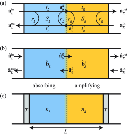
Figure 1: (Color online) Illustration of the wave-classical and quantum-optical treatment of $\mathcal{PT}$-symmetric systems, which are composed of an absorbing and an amplifying region. Panel (a) defines amplitudes used in the scattering approach to determine the resonance frequencies in the wave-classical limit (see Sec. II.1). Panel (b) defines the field operators for the quantum-optical input-output formalism of Sec. III. In panel (c) we sketch the quasi one-dimensional model resonator studied in Sec. V. This system is terminated by semitransparent mirrors with transmission probability $T$. In the interior, two regions of equal length $L/2$ are equipped with a refractive index $n_{L}$ (left region) and $n_{R}$ (right region), which is constant throughout each respective region. $\mathcal{PT}$ symmetry is realized for $n_{R}=n_{L}^{*}$. We write $n_{L}=n_{0}(1+i\alpha)$, where $\alpha$ controls the degree of nonhermiticity.

II.1.2 Spectral properties of closed systems

Consider a closed resonator that is split (if only artificially) into two parts L and R (‘left’ and ‘right’), which are described by scattering matrices identical to the reflection blocks $r_{L}^{\prime}(\omega)$ and $r_{R}(\omega)$, respectively [see the central region in Fig. 1(a), ignoring for the moment any leakage from the system]. At the interface, amplitudes of modes travelling ‘to the right’ (i.e. from L to R) are collected into a vector ${\bf a}_{0}^{R}$, while those for modes travelling into the opposite direction are collected into a vector ${\bf a}_{0}^{L}$. The matching conditions

$${\bf a}_{0}^{R}=r_{L}^{\prime}(\omega){\bf a}_{0}^{L},\quad{\bf a}_{0}^{L}=r_{R}(\omega){\bf a}_{0}^{R}$$ (4)

are consistent if

$${\rm det}\,[r_{L}^{\prime}(\omega)r_{R}(\omega)-\openone]=0.$$ (5)

For a hermitian system, where the scattering matrices are unitary, this condition only admits real frequencies. In presence of absorption or amplification, however, where the scattering matrices are nonunitary, the eigenfrequencies generally are complex. In both cases, these solutions are identical to the eigenvalues of the (possibly nonhermitian) underlying Hamiltonian.

The interest in $\mathcal{PT}$ symmetry for nonhermitian systems arises because this provides a mechanism where at least part of the spectrum can still be real. In the scattering formalism, this is embodied by the relation H.Schomerus ; Y.D.Chong

$$r_{R}(\omega)=\mathcal{PT}r_{L}^{\prime}(\omega)=[\{r_{L}^{\prime}(\omega^{*})\}^{*}]^{-1}$$ (6)

between the scattering matrices, where the labels L and R now refer to the symmetry-related subsystems. The quantization condition can then be written as

$${\rm det}\,[\{r_{L}^{\prime}(\omega)\}^{*}-r_{L}^{\prime}(\omega^{*})]=0.$$ (7)

On the real frequency axis, this reduces to the condition H.Schomerus

$${\rm det}\,{\rm Im}\,r_{L}^{\prime}(\omega)=0,$$ (8)

which can be generically fulfilled by varying a single real parameter (i.e., $\omega$), as it involves the determinant of a manifestly real matrix. However, the quantization condition can also have complex solutions, which then occur in complex-conjugated pairs.

The transition between both situations involves pairs of frequencies that coalesce on the real axis, and then move into the complex plane, where they remain related by complex conjugation C.M.Bender1 ; M.Znojil ; A.Mostafazadeh ; A.Mostafazadeh0 ; C.M.Bender3 ; F.G.Scholtz ; S.Klaiman ; S.Bittner . Typically, this transition is driven by increasing the nonhermiticity (the trend does not need to be strict; sometimes pairs of resonance frequencies become real when the nonhermiticity is increased). However, the transition also depends on the coupling of the absorbing and amplifying regions, and indeed can be induced by reducing this coupling H.Schomerus3 ; O.Bendix ; C.T.West . (In the trivial limit where the two regions are decoupled, they both possess a fully complex spectrum.)

While ${\cal PT}$ symmetry leaves wavefunctions of real eigenvalues invariant, it interchanges those of complex-conjugated pairs, which are therefore not ${\cal PT}$-symmetric when taken each on their own C.M.Bender1 ; C.M.Bender3 . This entails that at the point of degeneracy the two wavefunctions have to collapse, thereby resulting in an exceptional point, which is the generic degeneracy scenario in nonhermitian systems T.Kato ; W.D.Heiss ; C.Dembowski ; M.V.Berry2 . For the case of the Helmholtz equation, this behavior can be quantified on the basis of the bi-orthogonality relation

$$\int n^{2}\psi_{1}\psi_{2}d{\bf r}=0,$$ (9)

which holds for any two resonance modes $\psi_{1}$, $\psi_{2}$, even if the refractive index is complex. As one approaches the exceptional point, $\psi_{2}\to\psi_{1}\equiv\psi$ is shared between the two degenerate eigenvalues, and the wave function becomes self-orthogonal,

$$\int n^{2}\psi^{2}d{\bf r}=0\quad\mbox{(exceptional point)}.$$ (10)

II.1.3 Spectral properties of open systems

For a leaky (geometrically open) system, such as a resonator confined by semitransparent mirrors, the eigenfrequencies are generally shifted into the complex plane, corresponding to resonance frequencies of quasibound states with decay rate $-2{\rm Im}\,\omega$. These quasibound states fulfill the wave equation with purely outgoing boundary conditions. For a passive system, their decay rates are positive. In the presence of amplification counteracting the leakage, individual resonances can cross from the lower to the upper half of the complex plane. This signifies an instability, which in optics corresponds to the laser threshold A.E.SiegmanBook ; H.Schomerus ; S.Longhi2 ; Y.D.Chong .

The complex resonance spectrum can again be obtained from scattering theory E.Doron . Including the leakage channels to the outside, the scattering matrices of the left and right parts assume a natural block structure

$$S_{L}=\left(\begin{array}[]{cc}r_{L}&t_{L}^{\prime}\\ t_{L}&r_{L}^{\prime}\\ \end{array}\right),\quad S_{R}=\left(\begin{array}[]{cc}r_{R}&t_{R}^{\prime}\\ t_{R}&r_{R}^{\prime}\\ \end{array}\right),$$ (11)

which now also contains scattering amplitudes related to reflection and transmission from and to the exterior regions [i.e., from the left and right entrances into these subsystems; see Fig. 1(a)]. The internal matching conditions still only involve the reflection blocks $r_{L}^{\prime}$ of the left system and $r_{R}$ of the right system, and thus remain of the form (4). Hence, the quantization condition is still given by Eq. (5). However, for the open system this condition typically admits only complex solutions, even if the underlying Hamiltonian is hermitian or ${\cal PT}$-symmetric.

From the perspective of the open system, the significance of Eq. (5) becomes clear when considering the composed scattering matrix $S=S_{L}\circ S_{R}$ of the total system, which is formed according to the matrix composition rule

$$\left(\begin{array}[]{cc}r_{L}&t_{L}^{\prime}\\ t_{L}&r_{L}^{\prime}\end{array}\right)\circ\left(\begin{array}[]{cc}r_{R}&t_{R}^{\prime}\\ t_{R}&r_{R}^{\prime}\end{array}\right)$$ (16)

$$=\left(\begin{array}[]{cc}r_{L}+t_{L}^{\prime}\frac{1}{1-r_{R}r_{L}^{\prime}}r_{R}t_{L}&t_{L}^{\prime}\frac{1}{1-r_{R}r_{L}^{\prime}}t_{R}^{\prime}\\ t_{R}\frac{1}{1-r_{L}^{\prime}r_{R}}t_{L}&r_{R}^{\prime}+t_{R}\frac{1}{1-r_{L}^{\prime}r_{R}}r_{L}^{\prime}t_{R}^{\prime}\end{array}\right).\qquad$$ (19)

These expressions contain the resonant denominators $1-r_{L}^{\prime}r_{R}$, and thus diverge when condition (5) is met.

In the $\mathcal{PT}$-symmetric case, the scattering matrices in Eq. (11) are furthermore related according to H.Schomerus

$$S_{R}(\omega)=\mathcal{PT}S_{L}(\omega)=\sigma_{x}[S_{L}^{*}(\omega^{*})]^{-1}\sigma_{x}$$

$$=\left.\left(\begin{array}[]{cc}\frac{1}{(r_{L}^{\prime}-t_{L}r_{L}^{-1}t_{L}^{\prime})^{*}}&[r_{L}^{\prime-1}t_{L}\frac{1}{t_{L}^{\prime}r_{L}^{{}^{\prime}-1}t_{L}-r_{L}}]^{*}\\[5.69046pt] {}[r_{L}^{-1}t_{L}^{\prime}\frac{1}{t_{L}r_{L}^{-1}t_{L}^{\prime}-r_{L}^{\prime}}]^{*}&\frac{1}{(r_{L}-t_{L}^{\prime}r_{L}^{\prime-1}t_{L})^{*}}\\ \end{array}\right)\right|_{\omega^{*}},\qquad$$ (22)

where $\sigma_{x}$ in the first line is a Pauli matrix, and the second line follows from block inversion formulas. The resonance condition can then be written in the form

$${\rm det}\,(r_{L}^{\prime}(\omega)-[r_{L}^{\prime}(\omega^{*})-t_{L}(\omega^{*})r_{L}^{-1}(\omega^{*})t_{L}^{\prime}(\omega^{*})]^{*})=0.$$ (23)

The quantization condition (8) in the closed system is recovered for $t_{L}=t_{L}^{\prime}=0$.

When the system is almost closed, the eigenfrequencies are only slightly shifted downwards into the complex plane. The transition of the spectrum from real to complex is then replaced by a spectral rearrangement in which complex resonance frequencies approach each other very closely by moving together roughly parallel to the real axis, and then depart from each other into the direction of the imaginary axis A.Guo ; S.Longhi2 ; Y.D.Chong . When two complex frequencies meet in an exact degeneracy, one again reaches an exceptional point, where the wavefunctions of two resonance modes collapse and become self-orthogonal, in accordance to Eq. (10).

II.2 Excess noise for purely amplifying resonators

A practical method to probe the spectrum of a resonator is to fill it with an active, amplifying medium and observe the ensuing emitted radiation intensity. Far above the lasing threshold, one then observes coherent radiation with a narrow Lorentzian emission line A.E.SiegmanBook

$$I(\omega)=\frac{1}{2\pi}I_{\textrm{total}}\frac{\Delta\omega}{(\omega-\omega_{0})^{2}+\Delta\omega^{2}/4},$$ (24)

where the line width $\Delta\omega$ is dictated by noise. For the reference point of an almost closed purely amplifying resonator (the prototypical good-cavity laser), the quantum limit of the line width is given by the Schawlow-Townes relation A.L.Schawlow

$$\Delta\omega=\Gamma^{2}/2I_{\textrm{total}},$$ (25)

where $I_{\textrm{total}}=\int I(\omega)\,d\omega$, while $\Gamma$ is the cold-cavity decay rate in the passive resonator [corresponding to a real refractive index in Eq. (1)]. This noise is due to spontaneous emission events, which are incoherent and result in phase fluctuations, while amplitude fluctuations are suppressed by the feedback from the medium A.E.SiegmanBook ; P.Goldberg . In the linear regime just below the lasing threshold, on the other hand, where the emitted radiation is incoherent, amplitude and phase fluctuations are both present and equal each other, so that the Schawlow-Townes relation reads

$$\Delta\omega=\Gamma^{2}/I_{\textrm{total}}.$$ (26)

Both versions of the Schawlow-Townes relation require absence of absorption and assume orthogonal resonator modes, so that crosstalk between photons emitted into different modes can be ignored. In order to identify corrections due to the violation of these assumptions, it is advantageous to concentrate on the linear regime just below threshold, where the emitted intensity can be calculated conveniently in the scattering input-output formalism M.J.Collett ; T.Gruner ; C.W.J.Beenakker . Results can be translated to the lasing regime by the simple rule that there the quantum-limited line width is still reduced by a factor of two P.Goldberg . In the remainder of the background section we collect results for the previously studied case of purely amplifying systems K.Petermann ; A.E.Siegman ; P.Goldberg ; G.H.C.New ; M.Patra ; H.Schomerus1 , focussing only on some key points as the details of the derivation are encompassed by our more general considerations in Secs. III and IV.

The formalism starts with the classical wave equation, e.g., the Helmholtz equation (1). For a passive system (with a real refractive index) the scattering matrix $S(\omega)$ is unitary, $SS^{\dagger}=\openone$, but in presence of amplification this condition no longer holds. A physical consequence is the appearance of quantum noise. When amplitudes are promoted to annihilation operators $\hat{\bf a}^{\rm in,out}$, Eq. (2) with nonunitary $S$ is not compatible with the bosonic commutation relations for both sets of operators. This problem can be fixed by introducing auxiliary bosonic operators $\hat{\bf b}$, such that

$$\hat{\bf a}^{\rm out}=S(\omega)\hat{\bf a}^{\rm in}+Q(\omega)\hat{\bf b}^{\dagger}.$$ (27)

The commutation relations for $\hat{\bf a}^{\rm in}$ and $\hat{\bf a}^{\rm out}$ are now compatible if $SS^{\dagger}-QQ^{\dagger}=\openone$. This constraint has the status of a fluctuation-dissipation theorem. It admits solutions when $Q$ is equipped with at least as many columns as rows, but does not fix $Q$ completely. However, subject to reasonable physical assumptions, the constraint is sufficient to calculate the output intensity of the system in terms of its classical wave scattering properties.

For illustration we consider the case of total population inversion ($\langle\hat{\bf b}^{\dagger}\hat{\bf b}\rangle=0$) and no incoming radiation. The frequency-resolved output intensity is then of the form M.Patra

$$I(\omega)=\frac{1}{2\pi}\langle\hat{\bf a}^{{\rm out}\dagger}\hat{\bf a}^{\rm out}\rangle=\frac{1}{2\pi}{\rm tr}\,QQ^{\dagger}=\frac{1}{2\pi}{\rm tr}\,(SS^{\dagger}-\openone).$$ (28)

The final expression no longer contains the matrix $Q$ and therefore can be calculated purely based on the classical wave problem. In the vicinity of resonant emission frequencies, where the scattering matrix diverges [see Eqs. (5) and (19)], the radiated intensity is large. Linearizing in the deviation from the resonance condition, one generally finds a Lorentzian line shape

$$I(\omega)=\frac{K}{2\pi}\frac{\Gamma^{2}}{(\omega-\omega_{0})^{2}+\Delta\omega^{2}/4},$$ (29)

which features an extra factor $K$ so that the Schawlow-Townes relation Eq. (26) is replaced by

$$\Delta\omega=K\Gamma^{2}/I_{\textrm{total}}.$$ (30)

The factor $K$ is known as the Petermann factor K.Petermann , and can often be related to mode nonorthogonality A.E.Siegman ; P.Goldberg ; G.H.C.New ; M.Patra ; H.Schomerus1 . For the Helmholtz equation (1), this factor takes the explicit form H.Schomerus1

$$K=\left|\frac{\int|\psi|^{2}{\rm Im}(n^{2})\,d{\bf r}}{\int\psi^{2}{\rm Im}(n^{2})\,d{\bf r}}\right|^{2},$$ (31)

which holds also in presence of inhomogeneity in the refractive index and the gain. For a homogeneously amplifying resonator, this reduces to Siegman’s original expression A.E.Siegman

$$K=\frac{|\int|\psi|^{2}d{\bf r}|^{2}}{|\int\psi^{2}d{\bf r}|^{2}}.$$ (32)

The connection of the excess noise to mode nonorthogonality becomes apparent when one considers the combination (see also Sec. IV) H.Schomerus1

$$K\Gamma^{2}\approx\omega_{0}^{2}\left|\frac{\int|\psi|^{2}{\rm Im}(n^{2})\,d{\bf r}}{\int\psi^{2}n^{2}\,d{\bf r}}\right|^{2},$$ (33)

which appears in the numerator of Eq. (29). The self-orthogonality condition (10) implies that this combination diverges at an exceptional point. In general, the integral in the denominator of Eq. (33) can be interpreted as a suitably weighted overlap integral of the left eigenfunction $\psi$ and the right eigenfunction $\psi^{*}$, which represents the scalar product between these two types of eigenfunction (the stated simple relation of left and right eigenfunctions holds because the potential in the Helmholtz equation is scalar, but breaks down in the presence of vector potentials B.Dietz2 ). Furthermore, expressions (31) and (32) both imply $K\geq 1$, where $K=1$ is only obtained in the limit of a passive, closed system, in which the wave function is real. In more physical terms, on the other hand, expression (31) signifies that the excess noise is generated in the amplifying parts of the system, since the passive parts (with real refractive index) do not contribute to the integrals.

Clearly, this duality of interpretations of the Petermann factor in terms of mode nonorthogonality and excess quantum noise breaks down in presence of absorbing parts of the system. The mode nonorthogonality is then also induced by the absorbing regions with a positive imaginary part of the refractive index, but these on their own do not create any radiation. One of the main goals of the present work is to identify the role of the Petermann factor in the presence of such absorbing elements. We focus on $\mathcal{PT}$-symmetric systems, as their peculiar spectral properties imply that one can also easily steer close to an exceptional point, and examine how the total output intensity is regularized despite a divergent Petermann factor. In the remainder of this paper, we therefore first set up a theory of quantum noise in simultaneous presence of absorbing and amplifying regions, and then identify signatures of nonhermiticity, mode-nonorthogonality, and exceptional points in the output radiation intensity, followed by an illustration for a specific $\mathcal{PT}$-symmetric system.

III Input-output formalism in the presence of absorbing regions

In this section we extend the scattering input-output formalism described in Sec. II.2 to systems which combine amplifying and absorbing regions.

In simultaneous presence of gain by amplification and loss by absorption, the input-output relations (27) modify into C.W.J.Beenakker

$$\hat{\bf a}^{\rm out}=S(\omega)\hat{\bf a}^{\rm in}+Q_{(l)}(\omega)\hat{\bf b}_{(l)}+Q_{(g)}(\omega)\hat{\bf b}_{(g)}^{\dagger},$$ (34)

where $(l)$ refers to the absorbing (lossy) regions and $(g)$ refers to the amplifying regions (with gain). The commutation relations now deliver the constraint $SS^{\dagger}+Q_{(l)}Q_{(l)}^{\dagger}-Q_{(g)}Q_{(g)}^{\dagger}=\openone$, which no longer uniquely relates the coupling strengths (encoded in the combinations $QQ^{\dagger}$) to the deviation of the scattering matrix from unitarity.

In order to circumvent this problem, we assume that the absorbing and amplifying regions are spatially separated. For $\mathcal{PT}$-symmetric systems, this assumption is rather natural, as the $\mathcal{P}$ symmetry is usually of a geometric nature, such as a reflection $x\to-x$ about a plane perpendicular to the $x$-axis. To be specific, we assign absorption to the left part of the system and amplification to the right part of the system [see Fig. 1(b)]. This strategy, briefly sketched and applied to a special case in Ref. H.Schomerus , works whenever a similar separation into different regions is present due to the physical composition of the system, even in absence of symmetries. We therefore consider this slightly more general case, i.e., we first only assume that the absorbing and amplifying parts can be separated, and only then impose symmetry relations between them.

The classical wave scattering from the right and left parts is described by the scattering matrices $S_{L}$ and $S_{R}$, whose natural block structure given in Eq. (11). The corresponding input-output relations read

$$\left(\begin{array}[]{c}\hat{\bf a}_{L}^{\rm out}\\ \hat{\bf a}_{0}^{R}\end{array}\right) = S_{L}\left(\begin{array}[]{c}\hat{\bf a}_{L}^{\rm in}\\ \hat{\bf a}_{0}^{L}\end{array}\right)+\left(\begin{array}[]{c}Q_{L}\\ Q_{L}^{\prime}\end{array}\right)\hat{\bf b}_{L},$$ (35g)

$$\left(\begin{array}[]{c}\hat{\bf a}_{0}^{L}\\ \hat{\bf a}_{R}^{\rm out}\end{array}\right) = S_{R}\left(\begin{array}[]{c}\hat{\bf a}_{0}^{R}\\ \hat{\bf a}_{R}^{\rm in}\end{array}\right)+\left(\begin{array}[]{c}Q_{R}\\ Q_{R}^{\prime}\end{array}\right)\hat{\bf b}_{R}^{\dagger},$$ (35n)

where the various vectors of operators are defined in Fig. 1(b). Based on their commutation relations, the coupling strengths to the medium,

$$\left(\begin{array}[]{c}Q_{L}\\ Q_{L}^{\prime}\end{array}\right)(Q_{L}^{\dagger},Q_{L}^{\prime\dagger})=\openone-S_{L}S_{L}^{\dagger},$$ (36c)

$$\left(\begin{array}[]{c}Q_{R}\\ Q_{R}^{\prime}\end{array}\right)(Q_{R}^{\dagger},Q_{R}^{\prime\dagger})=S_{R}S_{R}^{\dagger}-\openone,$$ (36f)

are now again related to the scattering properties of the purely absorbing or amplifying parts of the system. As in the derivation of Eq. (28), the relations (36) are sufficient to calculate the output radiation of the system in terms of the classical scattering properties encoded in $S_{L}$ and $S_{R}$.

Starting from the relations (35), we algebraically eliminate the auxiliary operators $\hat{\bf a}_{0}^{L}$ and $\hat{\bf a}_{0}^{R}$ at the interface between the two regions,

$$\hat{\bf a}_{0}^{L}=\frac{1}{1-r_{R}r_{L}^{\prime}}[t_{R}^{\prime}\hat{\bf a}_{R}^{\rm in}+r_{R}t_{L}\hat{\bf a}_{L}^{\rm in}+Q_{R}\hat{\bf b}_{R}^{\dagger}+r_{R}Q_{L}^{\prime}\hat{\bf b}_{L}],$$

(37a)

$$\hat{\bf a}_{0}^{R}=\frac{1}{1-r_{L}^{\prime}r_{R}}[t_{L}\hat{\bf a}_{L}^{\rm in}+r_{L}^{\prime}t_{R}^{\prime}\hat{\bf a}_{R}^{\rm in}+Q_{L}^{\prime}\hat{\bf b}_{L}+r_{L}^{\prime}Q_{R}\hat{\bf b}_{R}^{\dagger}].$$

The annihilation operators for outgoing radiation then follow by substituting these expressions into

$$\hat{\bf a}_{L}^{\rm out}=r_{L}\hat{\bf a}_{L}^{\rm in}+Q_{L}\hat{\bf b}_{L}+t_{L}^{\prime}\hat{\bf a}_{0}^{L},$$ (38a)

$$\hat{\bf a}_{R}^{\rm out}=r_{R}^{\prime}\hat{\bf a}_{R}^{\rm in}+Q_{R}^{\prime}\hat{\bf b}_{R}+t_{R}\hat{\bf a}_{0}^{R}.$$ (38b)

We are interested in the radiation intensity which originates from the system, i.e., in absence of external incoming radiation, and therefore demand

$$\langle\hat{\bf a}_{nL}^{{\rm in}\dagger}\hat{\bf a}_{nL}^{\rm in}\rangle=\langle\hat{\bf a}_{nR}^{{\rm in}\dagger}\hat{\bf a}_{nR}^{\rm in}\rangle=0$$ (39)

for all incoming modes $n$ (expectation values of all crossterms between different incoming modes also vanish). Within the medium, we assume mode-independent expectation values

$$\langle\hat{\bf b}_{nL}^{\dagger}\hat{\bf b}_{nL}\rangle=f_{L},\quad\langle\hat{\bf b}_{nR}\hat{\bf b}_{nR}^{\dagger}\rangle=f_{R},$$ (40)

which can be associated to the excited-state occupations $g_{L}=f_{L}/(1+2f_{L})$ in the absorbing and $g_{R}=f_{R}/(2f_{R}-1)$ in the population-inverted amplifying parts of the system, respectively.

Under these conditions, the frequency-dependent output intensity of the composed system, resolved depending on whether it eventually emerges from the absorbing or the amplifying part of the system, takes the form

$$I_{L}(\omega) = \frac{1}{2\pi}\langle\hat{\bf a}_{L}^{{\rm out}\dagger}\cdot\hat{\bf a}_{L}^{\rm out}\rangle$$ (41)

$$= \frac{f_{R}}{2\pi}{\rm tr}\,\left[t_{L}^{\prime}\frac{1}{1-r_{R}r_{L}^{\prime}}Q_{R}\right]^{\dagger}\left[t_{L}^{\prime}\frac{1}{1-r_{R}r_{L}^{\prime}}Q_{R}\right]$$

$$+ \frac{f_{L}}{2\pi}{\rm tr}\,\left[Q_{L}+t_{L}^{\prime}\frac{1}{1-r_{R}r_{L}^{\prime}}r_{R}Q_{L}^{\prime}\right]^{\dagger}$$

$$\quad\times\left[Q_{L}+t_{L}^{\prime}\frac{1}{1-r_{R}r_{L}^{\prime}}r_{R}Q_{L}^{\prime}\right],$$

$$I_{R}(\omega) = \frac{1}{2\pi}\langle\hat{\bf a}_{R}^{{\rm out}\dagger}\cdot\hat{\bf a}_{R}^{\rm out}\rangle$$ (42)

$$= \frac{f_{L}}{2\pi}{\rm tr}\,\left[t_{R}\frac{1}{1-r_{L}^{\prime}r_{R}}Q_{L}^{\prime}\right]^{\dagger}\left[t_{R}\frac{1}{1-r_{L}^{\prime}r_{R}}Q_{L}^{\prime}\right]$$

$$+ \frac{f_{R}}{2\pi}{\rm tr}\,\left[Q_{R}^{\prime}+t_{R}\frac{1}{1-r_{L}^{\prime}r_{R}}r_{L}^{\prime}Q_{R}\right]^{\dagger}$$

$$\quad\times\left[Q_{R}^{\prime}+t_{R}\frac{1}{1-r_{L}^{\prime}r_{R}}r_{L}^{\prime}Q_{R}\right],$$

where all combinations of $Q$ matrices are completely determined via the relations (36). These expressions imply the appearance of narrow emission lines for frequencies close to resonance, which occurs whenever the denominator $1-r_{L}^{\prime}r_{R}$ vanishes, in accordance to the classical-wave quantization condition (5).

For a quasi one-dimensional resonator, the transmission and reflection matrices reduce to complex numbers. Equations (41) and (42) then yield the following more compact expressions,

$$I_{L} = \frac{1}{2\pi}\frac{|t_{L}^{\prime}|^{2}(|r_{R}|^{2}+|t_{R}^{\prime}|^{2}-1)}{|1-r_{R}r_{L}^{\prime}|^{2}},$$ (43)

$$I_{R} = \frac{1}{2\pi}\left[\frac{|t_{R}r_{L}^{\prime}|^{2}(|r_{R}|^{2}+|t_{R}^{\prime}|^{2}-1)}{|1-r_{R}r_{L}^{\prime}|^{2}}+|t_{R}|^{2}+|r_{R}^{\prime}|^{2}-1\right.$$ (44)

$$\left.+2\,{\rm Re}\,\frac{t_{R}r_{L}^{\prime}(r_{R}t_{R}^{*}+t_{R}^{\prime}r_{R}^{\prime*})}{1-r_{L}^{\prime}r_{R}}\right],$$

where we now made explicit use of Eq. (36) and assumed idealized conditions with $f_{L}=0$ (ground state population in the absorbing parts) and $f_{R}=1$ (total population inversion in the amplifying parts). For $\mathcal{PT}$-symmetric resonators the amplitudes are again related by Eq. (22), and the resonance condition is given by Eq. (23).

IV Near-resonant radiation intensity and the role of the Petermann factor

Starting from Eqs. (43) and (44) for the emitted intensity from a quasi one-dimensional resonator, we now evaluate the total intensity $I=I_{L}+I_{R}$ close to resonance, $\omega\approx\omega_{0}\equiv{\rm Re}\,\omega_{m}$, where the complex resonance frequency $\omega_{m}$ fulfills $r_{L}^{\prime}(\omega_{m})r_{R}(\omega_{m})=1$ according to Eq. (5). Keeping only resonant terms we have

$$I(\omega)=\frac{1}{2\pi}\frac{|t_{R}|^{2}(|t_{L}^{\prime}|^{2}+|t_{R}r_{L}^{\prime}|^{2})}{|1-r_{L}^{\prime}r_{R}|^{2}}\frac{|r_{R}|^{2}+|t_{R}|^{2}-1}{|t_{R}|^{2}},$$ (45)

where we grouped the terms for later convenience. Our goal is to relate this expression to properties of the resonance wave function $\psi_{m}$, which fulfills the one-dimensional Helmholtz equation

$$\psi_{m}^{\prime\prime}+k_{m}^{2}n^{2}(x)\psi_{m}=0$$ (46)

(with $k_{m}=\omega_{m}/c$) subject to purely outgoing boundary conditions. The derivation proceeds by a number of technical steps which lead to a compact final result, Eq. (52) below.

IV.1 Near-resonant radiation intensity

For convenience, we normalize the resonance wave function such that in the free space ($n=1$) to the right of the resonator $\psi_{m}(x)=k_{m}^{-1/2}\exp(ik_{m}x)$. Furthermore, we also insert a zero-width layer with $n=1$ at the interface between the right and the left region, where the wave function then takes the form

$$\psi_{m}=t_{R}^{-1}\exp(ik_{m}x)k_{m}^{-1/2}+r_{R}t_{R}^{-1}\exp(-ik_{m}x)k_{m}^{-1/2}.$$ (47)

Here we expressed the amplitudes by the elements of the scattering matrix $S_{R}$, Eq. (11). Furthermore, in terms of elements of the scattering matrix $S_{L}$, the outgoing component in the free space to the left of the resonator is given by $\psi_{m}(x)=\alpha k_{m}^{-1/2}\exp(-ik_{m}x)$, where $\alpha=t_{L}^{\prime}/t_{R}r_{L}^{\prime}=r_{R}t_{L}^{\prime}/t_{R}$ (the latter equality follows from the resonance quantization condition).

We now evaluate a number of integrals using Eq. (46), integration by parts, the condition ${\rm Re}\,\omega_{m}\gg|{\rm Im}\,\omega_{m}|$, and boundary terms matching the stipulated outgoing wave amplitudes. Below, ${\cal L}$ denotes the left part of the resonator, and ${\cal R}$ denotes the right part of the resonator. We then have

$$-\int_{{\cal R}}{\rm Im}\,(k_{m}^{2}n^{2})|\psi_{m}|^{2}$$

$$=\int_{{\cal R}}{\rm Im}\,(\psi_{m}^{*}\psi_{m}^{\prime\prime})=\left.{\rm Im}\,(\psi_{m}^{*}\psi_{m}^{\prime})\right|_{\partial{\cal R}}$$

$$=\frac{|r_{R}|^{2}+|t_{R}|^{2}-1}{|t_{R}|^{2}}.$$ (48)

Analogously, upon extending the integral over the whole resonator

$$-\int_{{\cal R}+{\cal L}}{\rm Im}\,k_{m}^{2}n^{2}|\psi_{m}|^{2}=\frac{|t_{L}^{\prime}|^{2}+|t_{R}r_{L}^{\prime}|^{2}}{|t_{R}r_{L}^{\prime}|^{2}}.$$ (49)

Finally, we employ a similar integral to investigate the behavior of the wave function close to resonance, $\omega=kc\approx\omega_{0}$. Due to the detuning, the wave function then also possesses incoming components, but as long as the detuning is small the outgoing components remain approximately unchanged. Therefore, we can assume that to the left of the resonator, $\psi(x)\approx k_{m}^{-1/2}[\alpha\exp(-ik_{m}x)+\beta\exp(ik_{m}x)]$ with $\alpha$ as given before, while to the right $\psi(x)\approx k_{m}^{-1/2}[\exp(ik_{m}x)+\gamma\exp(-ik_{m}x)]$.

The incoming components of the wave function can now be extracted via the following sequence of steps (which starts by linearizing $k^{2}$ around resonance):

$$2k_{m}(k-k_{m})\int_{{\cal R}+{\cal L}}n^{2}\psi_{m}^{2}$$ (50)

$$\approx \int_{{\cal R}+{\cal L}}(k^{2}-k_{m}^{2})n^{2}\psi_{m}^{2}$$

$$\approx \int_{{\cal R}+{\cal L}}(k^{2}-k_{m}^{2})n^{2}\psi_{m}\psi$$

$$= \int_{{\cal R}+{\cal L}}(-\psi^{\prime\prime}\psi_{m}+\psi_{m}^{\prime\prime}\psi)$$

$$= \left.[-\psi^{\prime}\psi_{m}+\psi_{m}^{\prime}\psi]\right|_{\partial({\cal R}+{\cal L})}$$

$$= 2i(\alpha\beta+\gamma).$$

Furthermore, in terms of the scattering matrix of the whole system we have $r\beta+t^{\prime}\gamma=\alpha$ and $t\beta+r^{\prime}\gamma=1$, which determines the coefficients $\beta$ and $\gamma$. We can then employ the scattering matrix composition rules (19) to express these coefficients in terms of the elements of $S_{L}$ and $S_{R}$. Close to resonance, this reduces to

$$(\alpha\beta+\gamma)\to-1/r^{\prime}\approx-(1-r_{L}^{\prime}r_{R})/(r_{L}^{\prime}t_{R}^{2}).$$ (51)

Based on expressions (48), (49), and (50), the near-resonant radiation intensity (45) can now be rewritten as

$$I(\omega) = \frac{1}{2\pi}\frac{\int_{{\cal R}}{\rm Im}\,\omega_{m}^{2}n^{2}|\psi_{m}|^{2}\int_{{\cal R}+{\cal L}}{\rm Im}\,\omega_{m}^{2}n^{2}|\psi_{m}|^{2}}{|\int_{{\cal R}+{\cal L}}\omega_{m}^{2}n^{2}\psi_{m}^{2}|^{2}}$$ (52)

$${}\times\frac{\omega_{0}^{2}}{(\omega-\omega_{0})^{2}+\Delta\omega^{2}/4}.$$

This is the central general result in this work. It applies to systems with amplifying and absorbing regions, including ${\cal PT}$-symmetric and purely amplifying systems, as is discussed in detail in the next subsection. The last factor is a Lorentzian of width $\Delta\omega=|2\,{\rm Im}\,\omega_{m}|$, centered at $\omega_{0}=\,{\rm Re}\,\omega_{m}$. The remaining combination of integrals resembles the expression (33) for a purely amplifying system. However, one of the integrals in the numerator extends over the whole system (where hermiticity is broken), while the other is restricted to the (amplifying) right part of the resonator. Therefore, this expression presents a mixture of the dual interpretations of the conventional Petermann factor as a measure of mode nonorthogonality and excess noise. Furthermore, as in Eq. (33) the denominator involves the appropriate overlap integral, which diverges at an exceptional point as a consequence of the self-orthogonality relation (10).

IV.2 Purely amplifying versus ${\cal PT}$-symmetric systems

In order to get a hold of the general features encoded in the near-resonant intensity (52), we first describe how one recovers from this expression the Petermann factor (31) for a purely amplifying resonator. In such a system, the breaking of hermiticity via the gain (encoded in ${\rm Im}\,n<0$) is constrained because this systematically shifts the resonances upwards in the complex plane. Therefore, the system is driven to the lasing threshold, which is reached when a resonance approaches the real axis. For highly excited modes (with large $\omega_{0}$), this happens very quickly, for $|{\rm Im}\,n|\sim(\Gamma/\omega_{0}){\rm Re}\,n\ll{\rm Re}\,n$, where $\Gamma$ is the cold-cavity rate. One then can use perturbation theory to relate the required gain to $\Gamma$ via note1

$$\frac{\Gamma}{\omega_{0}}\approx\left|\frac{\int{\rm Im}\,(\omega_{m}^{2}n^{2})\psi_{m}^{2}}{\int\omega_{m}^{2}n^{2}\psi_{m}^{2}}\right|\qquad\mbox{\parbox{99.58464pt}{(purely amplifying resonator at threshold).}}$$ (53)

Here, the refractive index is no longer arbitrary but has to be chosen such that the resonator is at threshold. With the help of this relation, Eq. (52) turns into Eq. (29), recovering the Petermann factor $K$ as defined in (31).

For systems that are not purely amplifying, on the other hand, the breaking of hermiticity does not cause a systematic shift of resonances, as the absorbing regions counteract the effect of the amplifying regions. In comparison to the Lorentzian (29), one could then define a generalized Petermann factor as

$$K=\frac{\int_{{\cal R}}{\rm Im}\,(\omega_{m}^{2}n^{2})|\psi_{m}|^{2}\int_{{\cal R}+{\cal L}}{\rm Im}\,(\omega_{m}^{2}n^{2})|\psi_{m}|^{2}}{|\int_{{\cal R}+{\cal L}}\omega_{m}^{2}n^{2}\psi_{m}^{2}|^{2}}\frac{\omega_{0}^{2}}{\Gamma^{2}}.$$ (54)

The same perturbative treatment that leads to Eq. (53) entails more generally that the cold-cavity decay rate $\Gamma$ is related to the (measurable) line width $\Delta\omega=-2{\rm Im}\,\omega$ according to

$$\frac{\Gamma}{\omega_{0}}=\frac{\Delta\omega}{\omega_{0}}+\left|\frac{\int{\rm Im}\,(\omega_{m}^{2}n^{2})\psi_{m}^{2}}{\int\omega_{m}^{2}n^{2}\psi_{m}^{2}}\right|\quad\mbox{\parbox{102.43008pt}{(absorbing \& amplifying resonator, not necessarily at threshold).}}$$ (55)

[Equation (53) follows by demanding $\Delta\omega\ll\Gamma$ close to threshold.]

For the specific case of a $\mathcal{PT}$-symmetric resonator, the validity of this perturbative treatment is limited to the regime before the exceptional point, as such a point induces degeneracy, and the self-orthogonality property (10) implies that the denominator in Eq. (55) diverges. Before one reaches the exceptional point, however, the individual wave functions are $\mathcal{PT}$-symmetric, so that the integral in the numerator of Eq. (55) vanishes. Therefore, one can safely approximate

$$\Gamma=\Delta\omega\qquad\mbox{\parbox{128.0374pt}{($\mathcal{PT}$-symmetric resonators),}}$$ (56)

which in practice should hold up to very close to the exceptional point. Beyond the exceptional point, it should initially be reasonable to approximate $\Gamma$ by the average width the two involved, overlapping resonances. Typically (and as we will confirm below), the regime far beyond the exceptional point is physically inaccessible as one quickly reaches the laser threshold Y.D.Chong . Based on these observations, Eq. (52) can be directly applied to specific $\mathcal{PT}$-symmetric systems, which we illustrate in the next section for the example of a quasi one-dimensional resonator setup.

V Application to a $\mathcal{PT}$-symmetric resonator

V.1 Model system set-up

We now consider a specific $\mathcal{PT}$-symmetric resonator [depicted in Fig. 1(c)], which is made of two regions of equal length $L/2$ (i.e., the total resonator length is $L$). In the left (absorbing) part of the system, the complex refractive index $n_{L}=n_{0}+in_{I}$ ($n_{I}>0$), while $n_{R}=n_{L}^{*}=n_{0}-in_{I}$ in the right (amplifying) part of the system. The resonator is terminated by two identical semitransparent mirrors of transmission probability $T$. This resonator can be interpreted as an open version of the system studied in Ref. M.Znojil . It is also similar to the resonator studied in Ref. H.Schomerus , but features some backscattering at the interface between the regions due to the step in ${\rm Im}\,n$. Furthermore, apart from the additional mirrors, it is like the resonator studied in Ref. Y.D.Chong . These slight modifications are motivated by specific requirements for our investigation. The system must be open to study the output radiation, the backscattering facilitates the appearance of exceptional points, and the mirrors allow to study the limit $T\to 0$ of an almost closed resonator. Furthermore, the degree of nonhermiticity can be controlled by changing $n_{I}$.

V.2 Resonance frequencies and exceptional points

In order to obtain the resonance frequencies we apply the scattering quantization formalism of Sec. II.1. We compose the scattering matrices $S_{L}$ and $S_{R}$ from the scattering matrix

$$S_{T}=\left(\begin{array}[]{cc}-\sqrt{1-T}&-i\sqrt{T}\\ -i\sqrt{T}&-\sqrt{1-T}\end{array}\right)$$ (57)

of a semitransparent mirror with transmission probability $T$, the scattering matrix

$$S_{n_{1},n_{2}}=\frac{1}{n_{1}+n_{2}}\left(\begin{array}[]{cc}n_{1}-n_{2}&2\sqrt{n_{1}n_{2}}\\ 2\sqrt{n_{1}n_{2}}&n_{2}-n_{1}\end{array}\right)$$ (58)

for a refractive index step from $n_{1}$ to $n_{2}$, and the scattering matrix

$$S_{n}=\left(\begin{array}[]{cc}0&\exp(i\omega nL/2c)\\ \exp(i\omega nL/2c)&0\end{array}\right)$$ (59)

for ballistic propagation through a segment of refractive index $n$ and length $L/2$. Then note2

$$S_{L} = S_{T}\circ S_{1,n_{L}}\circ S_{n_{L}}\circ S_{n_{L},1},$$ (60a)

$$S_{R} = S_{1,n_{R}}\circ S_{n_{R}}\circ S_{n_{R},1}\circ S_{T},$$ (60b)

with matrix composition rule (19).

Following this prescription, we obtain the elements of $S_{L}$ in the form

$$r_{L}=-\frac{(n_{L}+1)A_{L}^{+}+(n_{L}-1)A_{L}^{-}X_{L}^{2}}{(n_{L}+1)A_{L}^{-}+(n_{L}-1)A_{L}^{+}X_{L}^{2}},$$ (61a)

$$t_{L}^{\prime}=t_{L}=-\frac{2in_{L}\sqrt{T}X_{L}}{(n_{L}+1)A_{L}^{-}+(n_{L}-1)A_{L}^{+}X_{L}^{2}},$$ (61b)

$$r_{L}^{\prime}=-\frac{(n_{L}-1)A_{L}^{-}+(n_{L}+1)A_{L}^{+}X_{L}^{2}}{(n_{L}+1)A_{L}^{-}+(n_{L}-1)A_{L}^{+}X_{L}^{2}},$$ (61c)

where we introduced

$$A_{L}^{\sigma}=\frac{1}{2}[(1+\sigma n_{L})\sqrt{1-T}+1-\sigma n_{L}],\quad X_{L}=e^{i\omega n_{L}L/2c}.$$ (62)

Analogously,

$$r_{R}=-\frac{(n_{R}-1)A_{R}^{-}+(n_{R}+1)A_{R}^{+}X_{R}^{2}}{(n_{R}+1)A_{R}^{-}+(n_{R}-1)A_{R}^{+}X_{R}^{2}},$$ (63a)

$$t_{R}^{\prime}=t_{R}=-\frac{2in_{R}\sqrt{T}X_{R}}{(n_{R}+1)A_{R}^{-}+(n_{R}-1)A_{R}^{+}X_{R}^{2}},$$ (63b)

$$r_{R}^{\prime}=-\frac{(n_{R}+1)A_{R}^{+}+(n_{R}-1)A_{R}^{-}X_{R}^{2}}{(n_{R}+1)A_{R}^{-}+(n_{R}-1)A_{R}^{+}X_{R}^{2}},$$ (63c)

where

$$A_{R}^{\sigma}=\frac{1}{2}[(1+\sigma n_{R})\sqrt{1-T}+1-\sigma n_{R}],\quad X_{R}=e^{i\omega n_{R}L/2c}.$$ (64)

We now apply the quantization condition (5). This delivers the equation

$$(n_{L}+n_{R})(A_{L}^{-}A_{R}^{-}-A_{L}^{+}A_{R}^{+}X_{L}^{2}X_{R}^{2})$$

$$=(n_{L}-n_{R})(A_{L}^{-}A_{R}^{+}X_{R}^{2}-A_{L}^{+}A_{R}^{-}X_{L}^{2}),$$ (65)

which has to be solved for the resonance frequencies entering via $X_{L}$ and $X_{R}$.

Equation (65) holds irrespective of whether the resonator is $\mathcal{PT}$-symmetric or not, but from now on we assume that this symmetry holds and therefore make use of $n_{R}=n_{L}^{*}=n_{0}-in_{I}$ and $A_{R}^{\pm}=(A_{L}^{\pm})^{*}$. Moreover, we introduce the scaled dimensionless frequency

$$\Omega=\omega n_{0}L/c$$ (66)

and the dimensionless degree of nonhermiticity

$$\alpha=n_{I}/n_{0}.$$ (67)

In terms of these quantities, we can rewrite Eq. (65) as

$$|A_{L}^{+}|^{2}e^{i\Omega}-|A_{L}^{-}|^{2}e^{-i\Omega}+i\alpha(A_{L}^{-}{A_{L}^{+}}^{*}e^{\alpha\Omega}-A_{L}^{+}{A_{L}^{-}}^{*}e^{-\alpha\Omega})=0.$$ (68)

V.2.1 Closed system

In the limit $T=0$ of a closed system, $A^{\pm}_{L,R}=1$. The quantization condition (68) then takes the form

$$\mathcal{F}(\Omega)\equiv\alpha\sinh(\alpha\Omega)+\sin(\Omega)=0,$$ (69)

which demands us to find the roots of a real function. The solutions are real, or occur in complex conjugated pairs, as required by $\mathcal{PT}$ symmetry. We denote these solutions as $\bar{\Omega}_{m}$ (where $m=1,2,3,\ldots$), so that we can refer back to them when we discuss the open system.

The transition from a real to a complex spectrum is driven by the degree of nonhermiticity $\alpha$. This transition involves exceptional points which occur when two real frequencies coalesce, delivering the additional condition

$$\mathcal{F}^{\prime}(\Omega)=\frac{\partial\mathcal{F}}{\partial\Omega}=\alpha^{2}\cosh(\alpha\Omega)+\cos(\Omega)=0.$$ (70)

For an exceptional point, Eqs. (69) and (70) have to be fulfilled simultaneously. We denote the corresponding value of $\alpha$ and the value $\bar{\Omega}$ of the two coalescing frequencies as $\alpha_{l}^{\star}$ and $\bar{\Omega}_{l}^{\star}$, respectively, where $l=1,2,3,\ldots$ enumerates the exceptional points. Equations (69) and (70) then are equivalent to the conditions

$$\cos(\bar{\Omega}_{l}^{\star})=-\alpha_{l}^{\star},\quad\cosh(\alpha_{l}^{\star}\bar{\Omega}_{l}^{\star})=1/\alpha_{l}^{\star}.$$ (71)

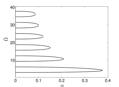
Figure 2: Illustration of spontaneous $\mathcal{PT}$-symmetry breaking in the model resonator of Fig. 1(c), for $T=0$ (closed system). The plot shows the dependence of the 12 lowest-lying dimensionless resonance frequencies $\bar{\Omega}$ on the hermiticity-breaking parameter $\alpha$, following their trajectory as long as they are real. As $\alpha$ increases, adjacent resonance frequencies approach each other pairwise, until they merge in an exceptional point. Beyond the exceptional point, the involved frequencies become a complex-conjugated pair, and then are no longer plotted. These results are obtained by numerical solution of Eq. (69).

For illustration, we plot in Fig. 2 a set of quantized frequencies as a function of $\alpha$, for a frequency range covering the 12 lowest-lying levels. The figure displays six exceptional points at which pairs of real frequencies coalesce. Beyond these points, the involved frequencies become complex, and then are no longer plotted.

For $\alpha=0$, the $m$th resonance frequency is located at $\bar{\Omega}_{m}=m\pi$ ($m=1,2,3,\ldots$). At the exception points two consecutive frequencies $\bar{\Omega}_{2l-1}$ and $\bar{\Omega}_{2l}$ approach the value $\bar{\Omega}_{l}^{\star}\approx 2l\pi-\pi/2$, an expression which becomes more and more accurate as $l$ increases. In the same limit, Eqs. (69) and (70) deliver the approximate condition

$$\alpha_{l}^{\star}e^{\alpha_{l}^{\star}\bar{\Omega}_{l}^{\star}}\approx 2.$$ (72)

With increasing $l$, $\alpha_{l}^{\star}$ decreases steadily, while the product $\alpha_{l}^{\star}\bar{\Omega}_{l}^{\star}$ increases very slowly.

In order to investigate the behaviour close to an exceptional point, we expand

$${\cal F}(\alpha,\Omega)\approx\frac{{\cal F}^{\prime\prime}(\alpha_{l}^{\star},\Omega_{l}^{\star})}{2}(\Omega-\Omega_{l}^{\star})^{2}+\dot{\cal F}(\alpha_{l}^{\star},\Omega_{l}^{\star})(\alpha-\alpha_{l}^{\star}),$$ (73)

where $\dot{\cal F}=\partial{\cal F}/\partial\alpha$, and we only kept the leading nonvanishing terms in this expansion. Slightly below the $l$th exceptional point, the two resonance frequencies are therefore given by

$$\bar{\Omega}_{2l}(\alpha) \approx \bar{\Omega}_{l}^{\star}+\sqrt{\frac{2\dot{\cal F}(\alpha_{l}^{\star},\Omega_{l}^{\star})}{{\cal F}^{\prime\prime}(\alpha_{l}^{\star},\Omega_{l}^{\star})}(\alpha_{l}^{\star}-\alpha)},$$ (74a)

$$\bar{\Omega}_{2l-1}(\alpha) \approx \bar{\Omega}_{l}^{\star}-\sqrt{\frac{2\dot{\cal F}(\alpha_{l}^{\star},\Omega_{l}^{\star})}{{\cal F}^{\prime\prime}(\alpha_{l}^{\star},\Omega_{l}^{\star})}(\alpha_{l}^{\star}-\alpha)}.$$ (74b)

Because of the square-root dependence, the spectral arrangement near the exceptional point occurs over a very small range of $\alpha$. In the following, we will use the term “far below (or above) the exceptional point” to indicate that the eigenvalues are well separated, while the regime where they are close together is called “slightly below (or above) the exceptional point”. However, in terms of numerical values $\alpha$ actually needs to approach $\alpha_{l}^{\star}$ very closely before the latter regime is entered. For later convenience we also note that by a similar expansion as in Eq. (73), the resonance splitting

$$\bar{\Omega}_{2l}(\alpha)-\bar{\Omega}_{2l-1}(\alpha) \approx 2\mathcal{F}^{\prime}(\alpha,\bar{\Omega}_{2l})/\mathcal{F}^{\prime\prime}(\alpha_{l}^{\star},\bar{\Omega}_{l}^{\star})$$ (75)

can be related to the deviation of $\mathcal{F}^{\prime}$ from the condition (70) for an exceptional point.

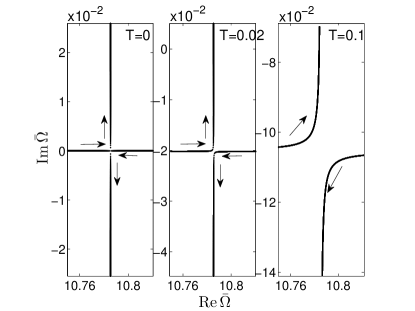
Figure 3: Evolution of a pair of dimensionless resonance frequencies in the complex plane, while sweeping the nonhermiticity parameter $\alpha$ of the $\mathcal{PT}$-symmetric model resonator depicted in Fig. 1(c). Shown are the resonance frequencies of the third and fourth level, with focus on the region around the exceptional point of the closed system ($T=0$, as realized in panel a). Panels $(b)$ and $(c)$ show the lifting of exact degeneracy when the system is slightly open ($T=0.02$ and $T=0.1$, respectively). The arrows indicate the direction of the evolution with increasing $\alpha$. Before the exceptional point, the resonances approach each other roughly parallel to the real frequency axis. Beyond the exceptional point, one of the two resonances is pushed towards the real axis, which facilitates the reaching of the lasing threshold (see Ref. Y.D.Chong for a system following the same scenario). These results are obtained by numerical solution of Eq. (68), where we set $n_{0}=2$.

V.2.2 Slightly open system

When the resonator is opened, bound states turn into quasibound states with complex resonance frequencies which are generally shifted by a mode-dependent amount downwards in the complex plane. For the system studied here, we find for $T\ll 1$ that this shift $\propto T$ is approximately rigid (i.e., mode independent), and is combined with a lifting $\sim T^{3/2}$ of resonance coalescence close to the exceptional points (to obtain exact coalescence in the complex plane, additional parameters beside $\alpha$ would have to be varied). These features follow by expanding the resonance condition (68) up to order $T^{2}$, upon which it takes the form

$$\mathcal{F}(\Omega)+i\frac{\Gamma_{0}}{2}\mathcal{F}^{\prime}(\Omega)-\alpha(1+\alpha^{2})\frac{\Gamma_{0}^{2}}{8}\sinh\alpha\Omega=0$$ (76)

where

$$\Gamma_{0}=\frac{n_{0}T}{1-T/2}.$$ (77)

To linear order in $\Gamma_{0}$, Eq. (76) is solved by

$$\Omega_{m}=\bar{\Omega}_{m}-i\Gamma_{0}/2,$$ (78)

where $\bar{\Omega}_{m}$ are the bound-state frequencies of the closed system, determined by Eq. (69). Slightly opening up this resonator thus does not change the real parts of the resonance frequencies, and shifts the imaginary parts by a mode-independent amount. In accordance to Eq. (56), this shift does not depend on the degree of nonhermiticity $\alpha$, which identifies $\Gamma_{0}$ as the cold-cavity decay rate. Notably, $\Gamma_{0}$ also determines the rigid shift of complex-conjugated pairs if $\mathcal{PT}$-symmetry in the closed system is spontaneously broken.

For illustration, we plot in Fig. 3 the evolution of two resonance frequencies in the complex plane while the parameter $\alpha$ passes through an exceptional point of the closed system. The arrows indicate the evolution direction of the resonance frequencies with increasing $\alpha$. We set $n_{0}=2$, such that the expected shift $\Gamma_{0}/2\approx T/(1-T/2)\approx T$ for small $T$. For the closed system (panel a), two real eigenvalues approach each other horizontally until they merge at the exceptional point, after with they become complex and move almost vertically away from each other. In panels (b) and (c), where the leakiness is small ($T=0.02$) and moderate ($T=0.1$), respectively, the resonance frequencies are shifted downwards by the expected amounts (for $T=0.1$, $T/(1-T/2)=0.105$, which corresponds well to the shift in the asymptotic regions to the left and right of the plotted range). The exceptional point is lifted only very slightly in panel (b), but much more distinctively in panel (c), and upon varying $T$ we find that the distance of closest approach in the complex plane is indeed of order $T^{3/2}$.

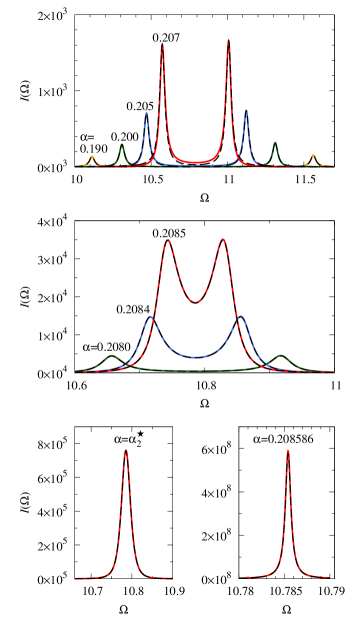
Figure 4: (Color online) Frequency-resolved intensity $I(\Omega)=I_{L}(\Omega)+I_{R}(\Omega)$ for the $\mathcal{PT}$-symmetric model resonator depicted in Fig. 1(c), for $n_{0}=2$ and $T=0.02$. Frequencies are in the range of the third and fourth resonance. Exact results from Eqs. (43) and Eq. (44) (solid curves) are compared with various approximations (dashed curves), as the nonhermiticity parameter $\alpha$ is changed to steer the system from the regime of well-isolated resonances across the exceptional point of the closed system ($\alpha_{2}^{\star}\approx 0.208573$) up to just below the lasing threshold (the threshold itself is at $\alpha\approx 0.208587$). Below the exceptional point (top panel), the isolated resonances agree with the Lorentzian lineshape (80). Slightly below the exceptional point (middle panel), the interfering resonances are well described by Eq. (84). This expression also holds true for $\alpha=\alpha_{2}^{\star}$, where Eq. (84) degenerates into the squared-Lorentzian (82) (lower left panel). Close to the lasing threshold one obtains again a Lorentzian line shape, in agreement with (85) (lower right panel). Note the dramatic increase in intensity as $\alpha$ is changed incrementally.

V.3 Frequency-resolved output radiation intensity

We now turn to the frequency-resolved output radiation intensities $I_{L}(\omega)$ and $I_{R}(\omega)$ from the left and right openings of the resonator. These follow by substituting the reflection and transmission amplitudes (61) and (63) into Eqs. (43) and (44), respectively. Since these expressions contain the general resonance quantization condition (5) in the denominator, the resonance frequencies calculated in the previous section determine the emission lines around which the output intensity is large. In this subsection, we directly derive expressions near resonance, including for the situation near an exceptional point; in the following subsection these are compared to the general near-resonant expression (52). For the discussion, we again make use of the dimensionless variables $\Omega$ and $\alpha$ [Eqs. (66) and (67), respectively].

Before we present analytical results, we illustrate the key features in Fig. 4, where the solid lines are numerical results for $I=I_{L}+I_{R}$, obtained from the expressions (43) and (44) as described above (the dashed lines represent analytical results derived below). We set $n_{0}=2$, $T=0.02$, and plot the intensity in a frequency range covering the third and the forth resonance, for values of $\alpha$ far below, near, and slightly beyond the exceptional point $\alpha_{2}^{\star}\approx 0.208573$ of the closed system (reaching up very closely to the lasing threshold, which occurs at $\alpha\approx 0.208587$).

The upper panel in Fig. 4 shows results for four values of $\alpha$ far below the exceptional point. The resonance frequencies are then well isolated, and the output intensity displays well-resolved resonance peaks which fit to a Lorentzian lineshape. As $\alpha$ increases, the resonances draw together and increase in height, but do not change their width, which is $\approx\Gamma_{0}$. The middle panel shows how resonances start to merge as one approaches the exceptional point. This goes along with a dramatically increasing intensity, which is in accordance to the expectation from strongly-violated mode orthogonality. At the exceptional point (lower left panel), the resonances merge into a very high single peak, which can be described by a squared Lorentzian, which still is of width $\sim\Gamma_{0}$. Moving beyond the exceptional point, the resonance peak retains its centre. As one approaches the lasing threshold (where one of the complex resonance frequencies approaches the real axis) the emission line reverts to a Lorentzian, and the peak intensity increases further while the resonance width decreases.

In order to explain these results we now obtain analytical expressions for the resonance peaks in the output intensity, covering the whole range far below, near and slightly beyond the exceptional point (where one quickly reaches the lasing threshold). On obtaining these expressions, it suffices to focus the attention on $I_{L}$, as $I_{R}$ leads to the same results in the relevant leading orders in $T$. The key step in the derivation is to approximate the resonant denominator in Eq. (43) by the same steps that lead from Eq. (68) to the simplified quantization condition (76). Applying similar (more straightforward) approximations also to the denominator, this leads to the expression

$$I_{L}(\Omega)=\frac{1}{2\pi}\frac{\Gamma_{0}}{2}\frac{(1+\alpha^{2})^{2}\sinh\alpha\Omega}{|\mathcal{F}(\Omega)+i\frac{\Gamma_{0}}{2}\mathcal{F}^{\prime}(\Omega)-\alpha(1+\alpha^{2})\frac{\Gamma_{0}^{2}}{8}\sinh\alpha\Omega|^{2}},$$ (79)

from which all subsequent results follow.

For an isolated resonance far below the exceptional point, we expand the denominator around the resonance condition $\Omega=\bar{\Omega}_{m}$, where $\bar{\Omega}_{m}$ is the real quantized frequency of the closed system, given by $\mathcal{F}=0$ [Eq. (69)]. This delivers the Lorentzian expression

$$I_{L}(\Omega)=\frac{1}{2\pi}\frac{(1+\alpha^{2})^{2}\sinh\alpha\bar{\Omega}_{m}}{\mathcal{F}^{\prime 2}(\bar{\Omega}_{m})}\frac{\Gamma_{0}/2}{(\Omega-\bar{\Omega}_{m})^{2}+\Gamma_{0}^{2}/4},$$ (80)

which in the upper panel of Fig. 4 is shown as a dashed line on top of the solid lines representing the exact numerical results. In the hermitian limit $\alpha\to 0$, $\mathcal{F}^{\prime}(\bar{\Omega}_{m})\to 1$, and

$$I_{L}(\Omega)\approx I_{L}^{(0)}(\Omega)\equiv\frac{1}{2\pi}\frac{\alpha\bar{\Omega}_{m}\Gamma_{0}/2}{(\Omega-\bar{\Omega}_{m})^{2}+\Gamma_{0}^{2}/4}.$$ (81)

As expected, Eq. (80) diverges at an exceptional point, which here is manifest because the term $\mathcal{F}^{\prime}(\bar{\Omega}_{m})$ then vanishes [see Eq. (70)]. This is remedied by keeping the next orders in the expansion of the denominator in Eq. (79), which results in the squared Lorentzian

$$I_{L}(\Omega) = \frac{1}{2\pi}\frac{(1+\alpha_{l}^{{\star}2})^{2}\sinh\alpha_{l}^{\star}\bar{\Omega}_{l}^{\star}}{\mathcal{F}^{\prime\prime 2}(\bar{\Omega}_{l}^{\star})}\frac{2\Gamma_{0}}{|(\Omega-\bar{\Omega}_{l}^{\star})^{2}+\Gamma_{0}^{2}/4|^{2}}$$ (82)

$$= \frac{1}{2\pi}\frac{1}{\alpha_{l}^{\star 2}\sinh\alpha_{l}^{\star}\bar{\Omega}_{l}^{\star}}\frac{2\Gamma_{0}}{|(\Omega-\bar{\Omega}_{l}^{\star})^{2}+\Gamma_{0}^{2}/4|^{2}},$$

where we used Eq. (69) to write

$$\mathcal{F}^{\prime\prime}(\Omega_{l}^{\star})=\alpha_{l}^{\star}(1+\alpha_{l}^{{\star}2})\sinh\alpha_{l}^{\star}\bar{\Omega}_{l}^{\star}.$$ (83)

Equation (82) is shown in the lower left panel of Fig. 4 as the dashed curve on top of the numerical result at the exceptional point.

In order to better understand the approach to this squared Lorentzian, let us rederive it by considering the merging of the two involved resonance frequencies $\bar{\Omega}_{2l-1}$ and $\bar{\Omega}_{2l}$ of the closed system. While each associated partial intensity diverges as one approaches the exceptional point, their coherent sum

$$I_{L}(\Omega)\approx\frac{1}{2\pi}\frac{\Gamma_{0}}{2}\frac{(1+\alpha_{l}^{{\star}2})^{2}\sinh\alpha_{l}^{\star}\bar{\Omega}_{l}^{\star}}{\mathcal{F}^{\prime 2}(\alpha,\bar{\Omega}_{2l})}$$

$$\qquad{}\times\left|\frac{1}{\Omega-\bar{\Omega}_{2l-1}+i\Gamma_{0}/2}-\frac{1}{\Omega-\bar{\Omega}_{2l}+i\Gamma_{0}/2}\right|^{2}$$

$$=\frac{1}{2\pi}\frac{1}{\alpha_{l}^{\star 2}\sinh\alpha_{l}^{\star}\bar{\Omega}_{l}^{\star}}\frac{2\Gamma_{0}}{|(\Omega-\bar{\Omega}_{2l-1}+i\frac{\Gamma_{0}}{2})(\Omega-\bar{\Omega}_{2l}+i\frac{\Gamma_{0}}{2})|^{2}}$$

(84)

[where we have made use of Eqs. (75) and (83)] remains finite, and reduces to the squared Lorentzian (82) when the two resonance frequencies coalesce. Expression (84) is also accurate slightly away from the exceptional point, as can be seen from the curves in the middle panel of Fig. 4.

Slightly beyond the exceptional point one approaches the lasing threshold, where one of the two resonances (with index $2l-1$ if continuously labeled as in Fig. 3) comes close to the real axis, thereby acquiring a much reduced width $\Delta\Omega=-2\,{\rm Im}\,\Omega_{2l-1}\approx\Gamma_{0}-2\,{\rm Im}\,\bar{\Omega}_{2l-1}\ll\Gamma$. The peak intensity of this resonance then exceeds by far that of the other resonance, resulting again in a (very narrow) Lorentzian

$$I_{L}(\Omega)=\frac{1}{2\pi}\frac{1}{\alpha_{l}^{\star 2}\sinh\alpha_{l}^{\star}\bar{\Omega}_{l}^{\star}}\frac{2/\Gamma_{0}}{(\Omega-{\rm Re}\,\bar{\Omega}_{2l-1})^{2}+\Delta\Omega^{2}/4}.$$ (85)

This is plotted in the bottom right panel of Fig. 4.

V.4 Implications of mode nonorthogonality

We now discuss the preceding analytical results for the model resonator from the perspective of mode nonorthogonality, based on the general considerations presented in Sec. IV. Our goal is to recover Eq. (80) by substituting the resonance wavefunction of the model system into Eq. (52).

Assuming no incoming radiation from the outside of the resonator, and employing scaled units $s=x/L$, the wave function in the left and right parts of the system (in which the respective refractive index is constant) can be written as

$$\psi_{L}=r_{n_{L},M}e^{i\Omega(1+i\alpha)(s+1/2)}+e^{-i\Omega(1+i\alpha)(s+1/2)},$$ (86a)

$$\psi_{R}=a[e^{i\Omega(1-i\alpha)(s-1/2)}+r_{n_{R},M}e^{-i\Omega(1-i\alpha)(s-1/2)}].\qquad$$ (86b)

Here

$$r_{n_{L},M}\approx-1+n_{L}T/2=-1+\frac{\Gamma_{0}}{2}(1+i\alpha),$$ (87a)

$$r_{n_{R},M}\approx-1+n_{R}T/2=-1+\frac{\Gamma_{0}}{2}(1-i\alpha),$$ (87b)

are the reflection coefficients of the mirrors, including the step in the refractive index from 1 to $n_{L}$ or $n_{R}$, respectively. The coefficient $a$ is determined by the matching condition $\psi_{L}(0)=\psi_{R}(0)$, giving for $\Gamma_{0}\to 0$

$$a=\frac{\sinh[i\Omega(1+i\alpha)/2]}{\sinh[i\Omega(1-i\alpha)/2]}.$$ (88)

The second matching condition $\psi_{L}^{\prime}(0)=\psi_{R}^{\prime}(0)$ recovers the quantization condition (69). From this, we only need the previously established property $\Omega_{m}\approx\bar{\Omega}_{m}-i\Gamma_{0}/2$ [Eq. (78)]. For $\Gamma_{0}\to 0$ and real $\Omega_{m}$, we furthermore find $|a|=1$.

Based on these expressions, and keeping only leading orders in $\Gamma_{0}$ (which also appears in $\Omega_{m}=\bar{\Omega}_{m}-i\Gamma_{0}/2$), as well as using the quantization condition (69), we find

$$\int_{{\cal R}}{\rm Im}\,\Omega_{m}^{2}n^{2}|\psi|^{2}=-2n_{0}^{2}(1+\alpha^{2})\bar{\Omega}_{m}\sinh(\alpha\bar{\Omega}_{m}),\qquad$$ (89a)

$$\int_{{\cal R}+{\cal L}}{\rm Im}\,\Omega_{m}^{2}n^{2}|\psi|^{2}=-2n_{0}^{2}(1+\alpha^{2})\bar{\Omega}_{m}\Gamma_{0},$$ (89b)

$$\left|\int_{{\cal R}+{\cal L}}\Omega_{m}^{2}n^{2}\psi^{2}\right|^{2}=[2\bar{\Omega}_{m}^{2}n_{0}^{2}{\cal F^{\prime}}(\bar{\Omega}_{m})]^{2}.$$ (89c)

Equation (52) then delivers

$$I(\Omega)=\frac{1}{2\pi}\frac{(1+\alpha^{2})^{2}\sinh(\alpha\bar{\Omega}_{m})}{{\cal F^{\prime}}^{2}(\bar{\Omega}_{m})}\frac{\Gamma_{0}}{(\Omega-\bar{\Omega}_{m})^{2}+\Gamma_{0}^{2}/4},$$ (90)

which indeed agrees exactly with our earlier result (80), given that $I_{L}=I_{R}=I/2$ in the considered regime $\Gamma_{0}\ll 1$. It is noteworthy that we explicitly recovered the term $\mathcal{F}^{\prime}$ in the denominator, which vanishes at an exceptional point. This confirms that the integral in the denominator of (52) constitutes the appropriate overlap integral, which quantifies the degree of mode nonorthogonality, as we already argued on general grounds in Sec. IV. Finally, we once more call attention to Eq. (84), which shows how the intensity is regularized by the interference of the near-degenerate resonances. In this construction, the partial amplitudes are still consistent with Eq. (90). We thus can conclude that the appearance of the squared-Lorentzian line shape at an exceptional point can be explicitly linked to the self-orthogonality property of the resonance wave function, Eq. (10).

VI Conclusions

Motivated by the recent interest in optical nonhermitian $\mathcal{PT}$-symmetric systems, we investigated the radiation intensity emitted by a resonator which is partially filled with an amplifying and an absorbing medium. This required to combine aspects of quantum noise with the properties of the resonator modes (especially, the consequences of broken hermiticity). We addressed these issues on the common basis of scattering theory, which allows to include quantum noise via the quantum-optical input-output formalism (see Secs. II.2 and III), while also giving access to the resonant frequencies (see Sec. II.1) and partial amplitudes in different regions of the resonator (see Sec. IV).

Our main result is an expression of the near-resonant frequency-resolved radiation intensity, Eq. (52), which relates this quantity to the properties of the resonant radiation mode, and includes an explicit measure of mode nonorthogonality induced by the amplifying and absorbing regions. $\mathcal{PT}$-symmetric systems provide natural access to exceptional points, where two resonances become degenerate, and their modes become self-orthogonal. The partial intensity of each resonance then diverges, but their sum yields a finite result, with a squared-Lorentzian line shape. Compared to the case of isolated resonances, we find that the total intensity is dramatically increased (see Fig. 4), which should facilitate the observation of this radiation in experiments.

We validated these results for the case of a model resonator (see Sec. V), for which we obtained explicit analytical results in the whole physically accessible range of broken hermiticity, from the case of isolated resonances [Eq. (80)] over the near-degenerate case close to an exceptional point [Eq. (84)] up to the lasing threshold [Eq. (85)].

- (1) R. El-Ganainy, K. G. Makris, D. N. Christodoulides, and Z. H. Musslimani, Opt. Lett. 32, 2632 (2007).
- (2) Z. H. Musslimani, K. G. Makris, R. El-Ganainy, and D. N. Christodoulides, Phys. Rev. Lett. 100, 030402 (2008).
- (3) K. G. Makris, R. El-Ganainy, D. N. Christodoulides, and Z. H. Musslimani, Phys. Rev. Lett. 100, 103904 (2008); Phys. Rev. A 81, 063807 (2010).
- (4) S. Longhi, Phys. Rev. Lett. 103, 123601 (2009); Phys. Rev. Lett. 105, 013903 (2010).
- (5) C. E. Rüter, K. G. Makris, R. El-Ganainy, D. N. Christodoulides, M. Segev, and D. Kip, Nature Phys. 6, 192 (2010).
- (6) A. Guo, G. J. Salamo, D. Duchesne, R. Morandotti, M. Volatier-Ravat, V. Aimez, G. A. Siviloglou, and D. N. Christodoulides, Phys. Rev. Lett. 103, 093902 (2010).
- (7) M. C. Zheng, D. N. Christodoulides, R. Fleischmann, and T. Kottos, Phys. Rev. A 82, 010103(R) (2010).
- (8) H. Ramezani, T. Kottos, R. El-Ganainy, and D. N. Christodoulides, Phys. Rev. A 82, 043803 (2010).
- (9) A. A. Sukhorukov, Z. Xu, and Y. S. Kivshar, Phys. Rev. A 82, 043818 (2010).
- (10) Z. Lin, H. Ramezani, T. Eichelkraut, T. Kottos, H. Cao, and D. N. Christodoulides, Phys. Rev. Lett. 106, 213901 (2011).
- (11) H. Schomerus, Phys. Rev. Lett. 104, 233601 (2010).
- (12) S. Longhi, Phys. Rev. A 82, 031801(R) (2010).
- (13) Y. D. Chong, L. Ge, and A. D. Stone, Phys. Rev. Lett. 106, 093902 (2011).
- (14) C. M. Bender and S. Boettcher, Phys. Rev. Lett. 80, 5243 (1998).
- (15) M. Znojil, Phys. Lett. A 285, 7 (2001).
- (16) A. Mostafazadeh, J. Math. Phys. (N.Y.) 43, 205 (2002); 43, 2814 (2002); 43, 3944 (2002).
- (17) A. Mostafazadeh and A. Batal, J. Phys. A: Math. Gen. 37, 11645 (2004).
- (18) C. M. Bender, Rep. Prog. Phys. 70, 947 (2007).
- (19) F. G. Scholtz, H. B. Geyer, and F. J. W. Hahne, Ann. Phys. (N.Y.) 213, 74 (1992).
- (20) S. Klaiman, U. Günther, and N. Moiseyev, Phys. Rev. Lett. 101, 080402 (2008).
- (21) S. Bittner, B. Dietz, U. Günther, H. L. Harney, M. Miski-Oglu, A. Richter, and F. Schäfer, preprint arXiv:1107.4256.
- (22) T. Kato, Perturbation theory for linear operators (Springer, Berlin, 1966).
- (23) W. D. Heiss, Phys. Rev. E 61, 929 (2000).
- (24) C. Dembowski, H. D. Gräf, H. L. Harney, A. Heine, W. D. Heiss, H. Rehfeld, and A. Richter, Phys. Rev. Lett. 86, 787 (2001).
- (25) M. V. Berry, J. Mod. Opt. 50, 63 (2003); Czech. J. Phys. 54, 1039 (2004).
- (26) S.-Y. Lee, J.-W. Ryu, J.-B. Shim, S.-B. Lee, S. W. Kim, and K. An, Phys. Rev. A 78, 015805 (2008); S.-B. Lee, J. Yang, S. Moon, S.-Y. Lee, J.-B. Shim, S. W. Kim, J.-H. Lee, and K. An, Phys. Rev. Lett. 103, 134101 (2009).
- (27) J. Wiersig, S. W. Kim, and M. Hentschel, Phys. Rev. A 78, 053809 (2008); J. Wiersig, A. Eberspächer, J.-B. Shim, J.-W. Ryu, S. Shinohara, M. Hentschel, and H. Schomerus, Phys. Rev. A 84, 023845 (2011).
- (28) J.-W. Ryu and S.-Y. Lee, Phys. Rev. E 83, 015203(R) (2011).
- (29) B. Dietz, H. L. Harney, O. N. Kirillov, M. Miski-Oglu, A. Richter, and F. Schäfer, Phys. Rev. Lett. 106, 150403 (2011).
- (30) L. Ge, Y. D. Chong, S. Rotter, H. E. Türeci, and A. D. Stone, Phys. Rev. A 84, 023820 (2011).
- (31) M. Liertzer, L. Ge, H. E. Türeci, and S. Rotter, preprint arXiv:1109.0454.
- (32) A. E. Siegman, Lasers (University Science Books, Mill Valley, CA, 1986).
- (33) A. L. Schawlow and C. H. Townes, Phys. Rev. 112, 1940 (1958).
- (34) K. Petermann, IEEE J. Quantum Electron 15, 566 (1979).
- (35) A. E. Siegman, Phys. Rev. A 39, 1253 (1989).
- (36) P. Goldberg, P. W. Milonni, and B. Sundaram, Phys. Rev. A 44, 1969 (1991).
- (37) G. H. C. New, J. Mod. Opt. 42, 799 (1995).
- (38) M. Patra, H. Schomerus, and C. W. J. Beenakker Phys. Rev. A 61, 023810 (2000); H. Schomerus, K. Frahm, M. Patra, and C.W. J. Beenakker, Physica A (Amsterdam) 278, 469 (2000).
- (39) H. Schomerus, Phys. Rev. A 79, 061801(R) (2009).
- (40) M. J. Collett and C. W. Gardiner, Phys. Rev. A 30, 1386 (1984); C. W. Gardiner and M. J. Collett, Phys. Rev. A 31, 3761 (1985).
- (41) T. Gruner and D.-G. Welsch, Phys. Rev. A 54, 1661 (1996).
- (42) C. W. J. Beenakker, Phys. Rev. Lett. 81, 1829 (1998).
- (43) A. Mondragón and E. Hernández, J. Phys. A 26, 5595 (1993); E. Hernández and A. Mondragón, Phys. Lett. B 326, 1 (1994).
- (44) N. J. Kylstra and C. J. Joachain, Phys. Rev. A 57, 412 (1998).
- (45) A. I. Magunov, I. Rotter, and S. I. Strakhova, J. Phys. B 34, 29 (2001).
- (46) Y. D. Chong, L. Ge, H. Cao, and A. D. Stone, Phys. Rev. Lett. 105, 053901 (2010).
- (47) J. Andreasen and H. Cao, Opt. Lett. 34, 3586 (2009); J. Andreasen, C. Vanneste, L. Ge, and H. Cao, Phys. Rev. A 81, 043818 (2010).
- (48) E. Doron and U. Smilansky, Nonlinearity 5, 1055 (1992).
- (49) E. B. Bogomolny, Nonlinearity 5, 805 (1992).
- (50) F. Cannata, J.-P. Dedonder, and A. Ventura, Ann. Phys. (N.Y.) 322, 397 (2007).
- (51) M. V. Berry, J. Phys. A 41, 244007 (2008).
- (52) H. F. Jones, Phys. Rev. D 76, 125003 (2007); 78, 065032 (2008).
- (53) H. Schomerus, Phys. Rev. A 83, 030101(R) (2011).
- (54) H. Hernandez-Coronado, D. Krejčiřík, and P. Siegl, Phys. Lett. A 375, 2149 (2011).
- (55) K. Abhinav, P. K. Panigrahi, and A. Jayannavar, preprint arXiv:1109.3113.
- (56) O. Bendix, R. Fleischmann, T. Kottos, and B. Shapiro, Phys. Rev. Lett. 103, 030402 (2009).
- (57) C. T. West, T. Kottos, and T. Prosen, Phys. Rev. Lett. 104, 054102 (2010).
- (58) This expression assumes that the amplification shifts the modes strictly upwards in the complex plane. For corrections due to the shift of the real part of the resonance frequency see Ref. H.Schomerus1 .
- (59) Note that for convenience we have inserted zero-width interfaces with refractive index between any two neighboring regions with different refractive index; this insertion does not alter the result.