The Lorentz-Dirac equation in complex space-time

Abstract

A hypothetical equation of motion is proposed for Kerr-Newman particles. It’s obtained by analytic continuation of the Lorentz-Dirac equation into complex space-time. A new class of “runaway” solutions are found which are similar to zitterbewegung. Electromagnetic fields generated by these motions are studied, and it’s found that the retarded (and advanced) times are multi-sheeted functions of the field points. This leads to non-uniqueness for the fields. With fixed weighting factors for these multiple roots, the solutions radiate. However, position dependent weighting factors can suppress radiation and allow non-radiating solutions. Motion with external forces are also considered, and radiation suppression is possible there too. These results are relevant for the idea that Kerr-Newman solutions provide insight into elementary particles and into emergent quantum mechanics. They illustrate a type of nascent wave-particle duality and complementarity in a purely classical field theory. Metric curvature due to gravitation is ignored.

1 Introduction

The Kerr-Newman (K-N) solutions of general relativity have been proposed as classical models for elementary particles burinskii_kerr_2007 ; burinskii_dirac_2008 ; carter_global_1968 ; lynden-bell_magic_2003 ; newman_classical_2002 ; pekeris_electromagnetic_1987 . Their gyromagnetic g factor is exactly 2, the same as the Dirac equation carter_global_1968 . It’s difficult to construct classical models with this property. One would like to know the equation of motion for such particles, but a rigorous derivation is lacking in the relativity literature. This paper proposes an equation of motion for them which is motivated by physical considerations, and then presents some properties and solutions. The method exploits the complex manifold techniques that have been prevalent in the literature on the K-N metric adamo_null_2009 ; newman_complex_1973 ; newman_heaven_1976 . There is recent renewed interest in the idea that quantum mechanics might be emergent from a simple, possibly deterministic dynamic at the Planck scale adler_quantum_2004 ; carroll_gravity_2004 ; markopoulou_quantum_2004 ; t_hooft_equivalence_1988 ; t_hooft_how_2001 ; t_hooft_determinism_2000 ; t_hooft_determinism_2005 ; t_hooft_entangled_2009 ; weinberg_collapse_2011 . A dynamical theory for the K-N particle could yield clues for this program. It has also been proposed that quantum mechanics might have emerged when the universe was in the ideal fluid mechanical phase, which is now believed to have occurred prior to about 3 microseconds after the big-bang davidson_quark-gluon_2008 ; davidson_quark-gluon_2010 , and where K-N particles might possibly have been formed due to turbulent density fluctuations in this fluid.

The Lorentz-Dirac equation (LDE) applies to exactly point-like classical charged particles in real Minkowski space. We study a complexified version of it, and find new solutions which are similar to zitterbewegung schroedinger_uber_1930 ; huang_zitterbewegung_1952 ; hestenes_zitterbewegung_1990 . These have unusual properties. The electromagnetic fields are not unique. Rather, an infinite number of possible fields can arise from a single particle solution. The origin of this is the multi-sheeted nature of the retarded time function. In fact, it has an infinite number of Riemann sheets. The null condition can be satisfied by an infinite number of different proper times for a given field point. This is radically different than ordinary classical electrodynamics, where only one unique single point can satisfy the retarded time condition. The multi-sheeted structure is analyzed here using mainly analytical but also numerical methods. The most general field solution is a linear superposition over all the possible retarded times, with weighting factors that are a countably infinite set of complex numbers (or even position dependent functions), and which are not determined by the theory. The situation bears a vague similarity to quantum mechanics, and even the many-worlds interpretation, where a state vector is associated with a particle and is required in order to specify the state of the particle. Here the state vector corresponds to the set of complex weights for the multitude of source points. The particle no longer acts as a single point or string so far as the electromagnetic field is concerned. This behavior is both intriguing but also very puzzling.

The treatment here is done in complex Minkowski space, and the gravitational interaction is ignored. A more rigorous and complete treatment would require the use of the Debney-Kerr-Schild formalism debney_solutions_1969 , which puts strong restrictions on the dynamics of the solutions by the extra requirement of the alignment of the Faraday tensor with the directions of the null congruence. It is well known that a relativistic quantum particle’s position cannot be localized with only positive energy states newton_localized_1949 ; wightman_localizability_1962 , and consequently a localized Schrödinger operator does not strictly speaking exist. Consequently second quantized field theory has been the central topic of modern particle physics for many years. However, modified and improved approaches to single particle relativistic wave equations have been proposed to remedy this situation prugovecki_consistent_1978 ; prugovecki_stochastic_1984 ; schroeck_quantum_1996 ; ali_conserved_1981 , and these “stochastic phase space” models may serve as a mathematical bridge between the current theory and the Dirac equation for example.

2 A brief overview of the Kerr-Newman solution and complex Minkowski space

The K-N particle is modeled as a point charge which is slightly displaced from the real space-time hypersurface embedded in complex Minkowski space (CM${}^{\text{4}}$) with corrections to the metric tensor due to gravity newman_metric_1965 ; newman_maxwells_1973 ; newman_complex_1973 ; newman_heaven_1976 ; burinskii_kerr_2007 ; burinskii_dirac_2008 ; lynden-bell_magic_2003 ; pekeris_electromagnetic_1987 . The gravitational and electromagnetic fields are singular on a ring and this endows the solution with string-like properties burinskii_gravitational_2011 . When the angular momentum is taken to zero, the ring collapses to a point singularity on the real Minkowski space as described by the Reissner–Nordström metric. When considered as a hypothetical model for an elementary particle, the gravitational effects are minute compared to electromagnetic ones burinskii_dirac_2008 , and shall be ignored here. However, the incorporation of the full metric calculation is extremely important for the ultimate importance of the ideas presented here, especially considering the complications and potential difficulties point out in burinskii_nonstationary_1995 for accelerated charges. It is hoped that by focusing first on the limiting electrodynamic theory the path to a full metric calculation will be illuminated. The complex theory makes contact with reality by ultimately considering the electromagnetic fields on the real space-time hyperspace. The Riemann-Silberstein complex vector field is used (we use boldface for 3-vectors and italics for 4-vectors and tensors)

$$\mathbf{W}=\mathbf{E}+i\mathbf{B}$$ (1)

or, in an equivalent covariant form, a complex Faraday tensor is introduced newman_maxwells_1973

$$W^{\mu\nu}=F^{\mu\nu}+i*F^{\mu\nu},\>*W=-iW$$ (2)

where $F$ is the Faraday tensor and $*F$ is the Hodge dual. $W$ is anti self-dual (ASD). The energy and momentum densities are

$$\mathcal{E}_{el}=\frac{1}{2}\overline{{\normalcolor\mathbf{W}}}\cdot\mathbf{W},\>\mathbf{P}_{el}=\frac{i}{2}\mathbf{W}\times\overline{\mathbf{W}}$$ (3)

The stress energy tensor on the real hyperspace is a function of the real-valued physical Faraday tensor

$$4\pi T^{\mu\nu}=F_{phys\>\lambda}^{\mu}F_{phys}^{\lambda\nu}+\frac{1}{4}g^{\mu\nu}F_{phys\alpha\beta}F_{phys}^{\alpha\beta}$$ (4)

and this can be expressed in terms of the complex Faraday tensor with the substitution

$$F_{phys}^{\mu\nu}=Re\>W^{\mu\nu}$$ (5)

The absence of magnetic charge requires that $F_{phys}$ satisfies the electromagnetic Bianchi identity, which is not automatically satisfied if $F$ is complex valued in (2), a problem taken up in section 8. The static K-N particle is modeled as a point charge located at a point in complex 3-space at $\mathbf{z_{0}}=\mathbf{x_{0}}+i\mathbf{b}$, where $\mathbf{x_{0}}$ and $\mathbf{b}$ are real 3-vectors. However, in many ways this object acts more like a string than a point charge burinskii_gravitational_2011 . One introduces a complex Coloumb potential

$$\Phi=q/\sqrt{\left(\mathbf{z}-\mathbf{z}_{0}\right)^{2}}$$ (6)

The complex vector inside the square root is simply squared and not absolute-value-squared in this equation, so that the resulting $\psi$ is complex even for real values of $\mathbf{z}$. $\Phi$ is holomorphic in each spatial coordinate and double-sheeted. It follows that $\nabla^{2}\Phi=0$ on the real hyperspace so long as $\mathbf{b}\neq 0$. The prescription for making physical sense out of this complex displacement is to take the Riemann-Silberstein vector as given by the analytic continuation of the electric field to complex values. Amazingly, this recipe yields the correct electromagnetic field of the K-N solution with $\mathbf{W}=-\mathbf{\nabla}\Phi$. The gradient is unambiguous because of the holomorphic property of $\Phi$, and its real and imaginary parts yield the electric and magnetic fields respectively. It also has two Riemann sheets because of the square root. As there is no charge on the real hyperspace when $\mathbf{z}_{0}$ is complex, this leads to the so-called “sourceless” K-N solution. The covariant version of this formula starts with a calculation of the analytic continuation of the real Faraday tensor to its value at the complex source point $\mathbf{z}_{0}$, $F_{c}^{\mu\nu}=\partial^{\mu}\Phi\delta^{0\nu}-\partial^{\nu}\Phi\delta^{0\mu}$, where $\delta$ denotes the Kronecker delta. This complex tensor will not be ASD automatically. In order to calculate the tensor $W$ we must use (2) to project out the ASD part. Then, on the real hypersapce, the real part will give the physical Faraday tensor (5).

The metric tensor is found by solving the equations of general relativity with a stress energy tensor given by (4), and by assuming that the metric can be expressed in Kerr-Schild coordinates in the form debney_solutions_1969 $g_{\mu\nu}=\eta_{\mu\nu}-2Hk_{\mu}k_{\nu}$, where $k$ is a null vector field, $H$ a scalar field, and $\eta$ is the Minkowski metric. The Kerr theorem provides a formula for the most general geodesic and shear-free congruences on real or complexified Minkowski space.

Introducing a discontinuity on the Riemann cut (which can be taken as the disk bounded by the ring singularity) leads to a surface charge and current density on this disk which can then be taken as a source for the fields which are made single valued but discontinuous by this procedure lynden-bell_electromagnetic_2004 . When considering values for charge, mass, and angular momentum (q, m, and j) of elementary particles, the gravitational metric is well-approximated by a Minkowski metric except very near to the ring singularity burinskii_dirac_2008 . The K-N solutions include the cases where the charge $q$ is complex. This describes particles with both an electric and magnetic charge calvani_latitudinal_1982 ; kasuya_exact_1982 . They also include the case where the mass is negative. The total electromagnetic energy stored in the static electric and magnetic fields of a K-N solution is infinite lynden-bell_magic_2003 . Despite the fact that the electromagnetic energy is infinite, the mass of the K-N particle is finite, and is arbitrary and unrelated to the electromagnetic energy. Consequently, we cannot interpret these solutions as purely electromagnetic particles in the limit $G\rightarrow 0$. Something must account for the cancellation of the infinite electrostatic energy to yield a finite mass, so the Poincaré stress problem for the classical electron persists for the static K-N particle as well. Along these lines, an interesting mechanism to render the energy finite by introducing Higgs fields and modifying the purely electromagnetic K-N stress-energy tensor was proposed in burinskii_regularized_2010 . The K-N solutions have event horizons whenever the mass is sufficiently large such that (in Planck units) $m^{2}>(j/m)^{2}+q^{2}$ burinskii_dirac_2008 ; carter_global_1968 . For the case of elementary particles, event horizons would not be present, and consequently the ring singularity would be naked. This violates the cosmic censorship hypothesis penrose_question_1999 , but whether this is sufficient reason to abandon consideration of such K-N particles is unclear at the present time. In the regularized solution of burinskii_regularized_2010 there is no singularity.

3 The Lorentz-Dirac equation (LDE)

The LDE for a single particle is dirac_classical_1938 ; jackson_classical_1999 ; plass_classical_1961 ; rohrlich_classical_2007 ; teitelboim_classical_1980

$$m_{0}a^{\mu}=F_{ext}^{\mu}+m_{0}\tau_{0}\left(\dot{a}^{\mu}+a^{\lambda}a_{\lambda}v^{\mu}\right)$$ (7)

where $F_{ext}^{\mu}$ is any external force, $\tau_{0}=\frac{2q_{0}^{2}}{3m_{0}c^{3}}$, and c=1, $a$ and $v$ are the proper acceleration and velocity respectively, and $\tau$ is the proper time. Einstein summation convention is assumed, and dot-product notation will be used for 4-vector dot products as well, so that $a^{\lambda}a_{\lambda}=a\cdot a$. The metric signature is (+,-,-,-). We use the notation $A^{[\mu}B^{\nu]}=A^{\mu}B^{\nu}-A^{\nu}B^{\mu}$. Boldface type will be used to denote 3-vectors, and their dot products will be as usual. For time-like particles, the equation is supplemented by subsidiary constraints on the proper acceleration and velocity which imply that in the rest frame, the acceleration 4-vector is space-like

$$v\cdot v=1,\;v\cdot a=0$$ (8)

The vast literature on this equation is reasonably in agreement on two points. First, if we consider exactly point particles and not extended quasi-particles, then the general consensus is that the LDE is correct in the sense that straightforward electromagnetic analysis leads to it. In fact it can be derived on purely geometrical grounds ringermacher_intrinsic_1979 . Secondly, this equation has one of two possible unphysical properties - either it has runaway solutions, or it has pre-acceleration. There is a tendency to replace the LDE in practical calculations by an approximate equation developed first by Landau and Lifshitz jackson_comment_2007 ; landau_classical_1951 which is suitable for non point-like quasi-particles and free of pathologies. Since the K-N solutions are obtained from a monopole in complex space-time, it is reasonable to consider the LDE and not the quasi-particle equation for describing them. The term $m\tau_{0}\dot{a}$ in (7) is called the Schott term. Its origin can be understood from the following equation for the total momentum of the charged particle including electromagnetic momentum teitelboim_splitting_1970 . $p^{\mu}=mv^{\mu}-\frac{2}{3}e^{2}a^{\mu}$ . The term $m\tau_{0}a^{2}v$ in (7) is the force caused by emitted radiation. In the method developed in this paper, the runaway solutions lead to interesting behavior, and therefore we study them in detail. It may turn out that this behavior will also be considered unphysical after further analysis, but in the meantime they are novel and seem worthy of study.

4 Runaway solutions

The most famous runaway solution of the LDE is rohrlich_classical_2007 for motion in the z-t plane

$$v^{\mu}=(cosh(Ae^{\tau/\tau_{0}}+B),\>0,\>0,\>sinh(Ae^{\tau/\tau_{0}}+B))^{\mu}$$ (9)

where $A$ and $B$ are constants. Let’s call these type I runaway solutions. Here the focus will be on another type of runaway solution. Consider the LDE, and Look for a solution which has vanishing acceleration squared in the absence of force

$$a^{\lambda}a_{\lambda}=0$$ (10)

then (7) becomes very simply $a^{\mu}=\tau_{0}\dot{a}^{\mu}$ with solution

$$a^{\mu}(\tau)=e^{\tau/\tau_{0}}a^{\mu}(0),\>a^{\lambda}(0)a_{\lambda}(0)=0$$ (11)

$$v^{\mu}(\tau)=\tau_{0}e^{\tau/\tau_{0}}a^{\mu}(0)+u^{\mu}$$ (12)

$$z^{\mu}(\tau)=\left(\tau_{0}\right)^{2}e^{\tau/\tau_{0}}a^{\mu}(0)+u^{\mu}\tau+\Omega^{\mu}$$ (13)

where $\Omega^{u}$ and $u^{\mu}$ are constant 4-vectors. For time-like particles, there are no non-trivial solutions which satisfy the constraints (8). In complex space-time, there are non-trivial solutions of this type, and these shall be the focus of this paper. These solutions shall be referred to as type II. Note that the Laplace transform in $\tau$ of a type II solution has a simple pole whereas the type I solutions have an infinite number of poles. So they are considerably simpler. Runaway solutions, dismissed as unphysical for over 100 years, have posed a profound challenge for classical electromagnetism. Note that both type I and II solutions are entire functions of $\tau$ if it is considered as a complex variable. They are also analytic functions of the constants of the motion $a^{\mu}(0)$, $\Omega^{\mu}$, and $u^{\mu}$.

5 Analytic continuation of free particle equation and solutions

The Free-particle LDE and its solutions can be analytically continued into the complex domain. We will let $\tau$, $z^{\mu}$ $a^{\mu}(0)$, $\Omega^{\mu}$, and $u^{\mu}$ all become complex variables. Considering first only the dependence on $\tau$, the position of the particle becomes not a curve but rather a two dimensional surface embedded in complex Minkowski space or CM${}^{\text{4}}$. This is because $\tau$ has both a real and imaginary part. Some of the literature has concluded that the particle acts like a string burinskii_gravitational_2011 . There is much merit in this string point of view, considering that the fields produced by the K-N solution are singular on a circular ring. Suppose we try and enforce that we have a point particle equation of motion by requiring that the particle move along a curve in complex space-time by constraining it to move along a curve in the complex $\tau$ plane. Let the curve be parametrized by some real variable $s$ so that the curve of the particle in complex Minkowski space is given by $z^{\mu}(\tau(s))$. The analytic continuation of the LDE and its solutions to complex $\tau$ are uniquely determined by their real hyperspace forms. We could interpret this as meaning that any analytic function $\tau(s)$ yields a possible solution for the charged particle’s motion due to self-forces while moving in complex space-time. One trajectory stands out in importance, and this is the one for which $z^{0}$, the time component, stays real along the trajectory. We think of this as the effective trajectory of the particle, while acknowledging the underlying string-like nature of the solution too burinskii_gravitational_2011 . Despite this non-uniqueness, one particular analytic continuation will be studied in detail here because of its similarity to zitterbewegung. Starting with all real values for the various initial parameters, set $\tau(s)=s$ for s real and ranging from $-\infty$ to $+\infty$ and then we analytically continue this curve to the curve $\tau(s)=is$ along the imaginary $\tau$ axis. An analytic transformation which accomplishes this is the following continuous function as $\lambda$ vary from 0 to 1.

$$\tau(\lambda,s)=s+(i-1)\lambda s,\>\lambda\in\left[0,1\right]$$ (14)

Actually, the reader may prefer to avoid trajectories altogether at this stage by simply making a change of complex variables $\tau=is$, but for the remainder of this section we shall restrict consideration to the trajectory mapped out by letting $s$ and $z^{0}$ vary along the real axis. Additional analytic continuations of the initial values $\Omega^{\mu},\>u^{\mu},\>a(0)^{\mu}$ will also be made in order to obtain a physically sensible solution. Applying (14) results in $\tau=is$ and consequently the LDE becomes

$$-m_{0}\frac{d^{2}z}{ds^{2}}^{\mu}=F_{ext}^{\mu}+im_{0}\tau_{0}\left(\frac{d^{3}z}{ds^{3}}^{\mu}-\left(\frac{d^{2}z}{ds^{2}}\right)^{2}\frac{dz}{ds}^{\mu}\right)$$ (15)

We wish to interpret $s$ as a new scaled proper time for the motion of the particle in the real hyperspace. This will allow us to fix some free parameters of the theory. Notice that then the inertial mass has the wrong sign though. A physical particle must have a positive inertial mass. The K-N metric has both positive and negative mass solutions, so we therefore choose $m_{0}$ to be negative. Note that if $m_{0}<0$ then $\tau_{0}$ changes sign too, so we have to take care with the signs. At the risk of confusion we will nevertheless continue to let $\tau_{0}$ denote the positive value. We have then, in the absence of external force

$$m\frac{d^{2}z}{ds^{2}}^{\mu}=im\tau_{0}\left(\frac{d^{3}z}{ds^{3}}^{\mu}-\left(\frac{d^{2}z}{ds^{2}}\right)^{2}\frac{dz}{ds}^{\mu}\right),\quad m=-m_{0}\>>0$$ (16)

The inertial and gravitational mass must be equal. We assume for the time being that this is possible with these assumptions, but to prove it would require solving for the gravitational metric which is difficult for the cases of interest considering burinskii_nonstationary_1995 . The change in sign for the mass might be due to some form of self interaction. Considering the type II runaway solutions (13) we have

$$a_{s}^{\mu}(s)=d^{2}z^{\mu}/ds^{2}=e^{-is/\tau_{0}}a_{s}^{\mu}(0),\quad a_{s}^{\lambda}(0)a_{s\lambda}(0)=0$$ (17)

$$v_{s}^{\mu}(s)=dz^{\mu}/ds=i\tau_{0}e^{-is/\tau_{0}}a_{s}^{\mu}(0)+V^{\mu}$$ (18)

$$z_{s}^{\mu}(s)=-\tau_{0}^{\,2}e^{-is/\tau_{0}}a_{s}^{\mu}(0)+V^{\mu}s+\Omega^{\mu}$$ (19)

and $V$ and $\Omega$ are constant 4-vectors, with $V$ real and time-like.

5.1 Circular rotating solution for free particles

Consider analytic continuation in the constant 4-vector $a_{s}(0)$ to the following pair of possible null vectors

$$a_{\pm}(0)=\delta_{a}(0,1,\pm i,0)$$ (20)

which will be seen to have opposite chirality. Although $\delta_{a}$ can be a complex constant, by choice of the zero point for $s$ we can absorb its phase, and so we take it to be real and positive. These null vectors lead to a localized oscillation in the complex space rather than a runaway solution. For future reference, the following formulas are easily verified

$$a_{\pm}(0)\cdot x=-\delta_{a}r_{\bot}e^{\pm i\varphi}$$ (21)

$$\left(Re\>a_{\pm}(0)\right)\cdot\left(Im\>a_{\pm}(0)\right)=0$$ (22)

where $r_{\bot}$and $\varphi$ are the radial and azimuthal coordinates for the 3-vector part of a real 4-vector $x$ in cylindrical coordinates. The most general solution of this type can be found by noting that an arbitrary complex 3-vector can be written $\mathbf{a_{s}(0)}=\mathbf{A}+i\mathbf{B}$ where $\mathbf{A}$ and $\mathbf{B}$ are real. Then, $\mathbf{a_{s}(0)^{2}}=0\Rightarrow\mathbf{A}\cdot\mathbf{B}=0$ and $\mathbf{A^{\mathrm{2}}}=\mathbf{B}^{2}$. These are all obtained from (20) the by a 3-rotation of $a_{\pm}(0)$. We let $\Omega^{\mu}$ have a small imaginary part to give it the properties of a spinning particle as dictated by the K-N static solution $\Omega^{\mu}=x_{0}^{\,\mu}+ib^{\mu}$, where $b^{\mu}$ is real and spacelike, and in the “average rest frame” where $V^{\mu}=(\gamma,0,0,0)$, $b^{\mu}=(0,\overrightarrow{b})$, and $\gamma$ is a real constant. In this example we have chosen to take $\vec{b}$ along the 3-direction to maintain symmetry. It might be oriented in other directions too, but these shall not be considered here. The magnitude of $\vec{b}$ is the angular momentum divided by mass for the K-N particle. For an electron, it would be $\hslash/2m_{e}$. We shall allow values of $\gamma\neq 1$ as this allows us to interpret the real part of $z_{s}$ as a true particle trajectory with proper time given by s. Note that $v_{s}\cdot v_{s}=\gamma^{2}\neq 1$, so this is a departure from ordinary classical mechanics. However, note also that with this complex acceleration, there is no rest frame for the particle which can be reached from the Laboratory frame with a real-valued Lorentz transformation. Writing out the real and imaginary parts in full (with $\delta_{a}$ real and positive and for $s$ real)

$$Re(z_{\pm}^{\mu})=-\tau_{0}^{2}\delta_{a}(0,\>cos(s/\tau_{0}),\>\pm sin(s/\tau_{0}),\>0)^{\mu}+V^{\mu}s+x_{0}^{\,\mu}$$ (23)

$$Im(z_{\pm}^{\mu})=-\tau_{0}^{2}\delta_{a}(0,\>-sin(s/\tau_{0}),\>\pm cos(s/\tau_{0}),\>0)^{\mu}+b^{\mu}$$ (24)

The real coordinates are the closest we can come describing this object as a normal particle. It is misleading to think that the particle is really a simple charge moving in a circle, just as the semiclassical interpretation of zitterbewegung in the Dirac equation as a circular particle motion is also a gross over-simplification. The proper velocity of the real trajectory is (for real values of $s$)

$$\frac{d}{ds}Re(z_{\pm}^{\mu})=-\tau_{0}\delta_{a}(0,\>-sin(s/\tau_{0}),\>\pm cos(s/\tau_{0}),\>0)^{\mu}+V^{\mu}$$ (25)

and this must satisfy

$$\frac{d}{ds}Re(z_{\pm}^{\mu})\frac{d}{ds}Re(z_{\pm\mu})=\gamma^{2}-(\tau_{0}\delta_{a})^{2}=1$$ (26)

which is required if this is to be interpreted as a time-like particle with $s$ its proper time. Therefore we must have $|\delta_{a}|=\sqrt{\gamma^{2}-1}/\tau_{0}$. It also follows for these solutions that

$$\left(\frac{d}{ds}z_{\pm}^{\mu}\right)a_{\pm\mu}=0\>,\mathrm{and}\>\left(\frac{d}{ds}Re(z_{\pm}^{\mu})\right)Re(a_{\pm\mu})=0$$ (27)

$$\left(dz/ds\right)^{2}=V^{\mu}V_{\mu}=\gamma^{2}$$ (28)

It is clear that the two solutions circulate with opposite chirality in the real hyperspace. The determination of a value to assign to $\gamma$ is not obvious. In order to fix it, we identify the oscillation with zitterbewegung as described by the Dirac equation dirac_principles_1978 ; schroedinger_uber_1930 ; huang_zitterbewegung_1952 ; barut_zitterbewegung_1981 ; hestenes_zitterbewegung_1990 which satisfies $\omega_{z}=2m_{obs}/\hslash$ where $m_{obs}$ is the positive physical mass of the observed particle, and the one to be used in the Dirac equation. Laboratory time is given by

$$t=Re\>z^{0}=V^{0}s=\gamma s$$ (29)

Expressing the oscillation in terms of this time, and equating it with the zitterbewegung angular frequency gives

$$e^{-is/\tau_{0}}=e^{-it/\gamma\tau_{0}}=e^{-i\omega_{z}t}=e^{-i(2m_{obs}/\hbar)t}$$ (30)

$$\frac{1}{\gamma\tau_{0}}=\omega_{z}=\frac{2m_{obs}}{\hbar},\>\tau_{0}=\frac{2q^{2}}{3m}$$ (31)

Considering (26), special relativity requires that the mechanical energy of the rotating point mass be $m_{obs}=\gamma m=\gamma|m_{0}|$ so that the observed mass must be different from the original static K-N mass in magnitude and sign. On combining these equations one finds that $\gamma$ is independent of mass and given by $\gamma^{2}=\frac{3\hslash}{4q^{2}}$. Introducing the fine structure constant $\alpha=\frac{e^{2}}{\hslash}$ we have for a particle with charge $e$

$$\gamma=\sqrt{\frac{3}{4\alpha}}=10.1378991576698\>\pm 1.66\times 10^{-8}$$ (32)

The uncertainty reflects the experimental uncertainty in $\alpha$. We’ve obtained this precise value of $\gamma$ by requiring that $s$ be the proper time of the projected real motion, and although this is a natural assumption, it’s not absolutely mandatory and one could consider other positive values for $\gamma$. We can interpret the solution as a particle with an internal clock which has twice the frequency as mandated by quantum mechanics - the de Broglie clock de_broglie_researches_1924 - which is the same as the result for the Dirac equation. In the average rest frame $Re\>z^{\mu}$ describes a circular orbit of radius $\tau_{0}^{2}\delta_{a}$ and angular frequency $\omega_{z}$. The laboratory speed, determined by the real part of $z$ is $\tau_{0}^{2}\mid\delta_{a}\mid\omega$. If we accept the usual arguments regarding zitterbewegung, then this would be the speed of light. This is only approximately true in our case. Solving (26) for $\delta$ yields $\delta_{a}=\sqrt{\gamma^{2}-1}/\tau_{0}$. The radius of oscillation is then approximately half of the (reduced) Compton wavelength $\lambda_{C}=2\gamma\tau_{0}$

$$r=\tau_{0}^{2}\delta_{a}=\tau_{0}\sqrt{\gamma^{2}-1}=\frac{\lambda_{C}\sqrt{\gamma^{2}-1}}{2\gamma}$$ (33)

so that the speed as viewed in the mean rest frame of the particle model for an electron is independent of mass and given by

$$r\omega_{z}=\sqrt{\gamma^{2}-1}/\gamma=(0.995123206731709\>\pm 1.60\times 10^{-11})c$$ (34)

In most models for zitterbewegung the speed is taken to be exactly c and the radius is given by schroedinger_uber_1930 ; barut_zitterbewegung_1981 ; hestenes_zitterbewegung_1990 $r_{S}=\frac{\hslash}{2m_{obs}}=\gamma\tau_{0}$. This value, originally due to Schrödinger, agrees with our radius to better than 1%. The angular momentum due to this circular motion alone may be calculated to be $L=\frac{\hbar}{2}\frac{\gamma^{2}-1}{\gamma^{2}}$. This is slightly smaller than the spin of the electron by about 1%. In addition to this purely mechanical angular momentum, there is also a contribution from the electromagnetic field angular momentum. It is hoped that this extra contribution will make up the deficit and yield a total angular moment of $\hbar/2$. These results are in qualitative agreement with zitterbewegung for the Dirac equation, but the speeds are subluminal here, and the real hyperspace projection of the particle’s world line describes a time-like particle. Underlying this apparent real motion though is a periodic null motion in complex space-time which was obtained by an analytic continuation of the LDE. The self-accelerating runaway solutions have been transformed by this procedure into localized oscillatory solutions, much like the zitterbewegung of the Dirac equation dirac_principles_1978 ; huang_zitterbewegung_1952 ; sidharth_revisiting_2008 ; hestenes_zitterbewegung_1990 . The physical existence of zitterbewegung has been experimentally verified through numerous spectroscopic calculations which need to include the Darwin term bjorken_relativistic_1998 to agree with experimental measurements of the hyperfine splitting of atomic lines in spectroscopy, and also more directly by observing resonant behavior in electron channeling guoanere_experimental_2008 . We’ve had to introduce mass renormalization, change the sign of the mass, and allow complex valued acceleration to have a plausible theory. The reward for these radical assumptions is that we have arrived at a solution to a purely classical equation which describes phenomenon that we actually observe in nature and which is normally associated with relativistic quantum mechanics. Moreover, the runaway solutions have been eliminated, without imposing the usual boundary condition that the acceleration vanish in the infinite future. In our case the acceleration endures forever, as does the zitterbewegung for a free Dirac particle. This explanation for zitterbewegung has a problem if neutrinos are included in the discussion, since if the mass of the neutrino is exactly zero, then $\tau_{0}$ would be undefined, but if its mass is non-zero, as is now believed, then $\tau_{0}=0$ and there would be no zitterbewegung. Many other solutions can be obtained from these ones by applying the full symmetry group of transformations for the complex LDE. This group includes as a subgroup the complex ten parameter Poincare group newman_complex_1973 ; streater_pct_2000 together with parity symmetry as well as complex conjugation of the initial acceleration 4-vector. Time reversal is not a symmetry of the LDE, presumably because a preferred direction in time is introduced in its derivation by allowing only the retarded fields to self-interact with the particle. Wheeler-Feynman electrodynamics wheeler_interaction_1945-1 in contrast is time symmetric. There is earlier literature showing a connection between the LDE and zitterbewegung as in browne_electron_1970-1 , but the relationship to the current theory is not clear at this time to the author.

5.2 space-time loop solution

Another class of solutions can be obtained by letting $a_{s}^{\mu}(0)=\delta_{03}(1,0,0,1)+\delta_{12}(0,1,\pm i,0)$ which is a null vector. This describes an additional oscillatory behavior in the z-t variables. If $a_{s}\cdot V=0$ then we must have $V^{\mu}=0$ if the mean 4-velocity is real and time-like, and we then get a closed loop in complex space-time. The motion is governed by arbitrary complex constants $\delta_{03}$ and $\delta_{12}$.

$$z_{s}(s)=-\tau_{0}^{\,2}e^{-is}\left[\delta_{03}(1,0,0,1)+\delta_{12}(0,1,\pm i,0)\right]+\Omega$$ (35)

Taking the real part of this yields circular oscillation in the 1-2 plane synchronized with linear oscillation in the 0-3 plane. As the time oscillates in this solution, it violates causality, although on a very tiny scale. The static K-N solutions are known to have time-like closed loop geodesics morris_wormholes_1988 ; morris_wormholes_1988-1 . This loop solution is qualitatively similar to a virtual particle loop in a Feynman diagram, and although we will not be considering these solutions further, they are pointed out here because of their possible relevance to emergent quantum mechanics. The most general complex null 4-vector $a_{s}(0)$ can be written as $a_{s}(0)=(\pm\sqrt{\mathbf{k\cdot k}},\>\mathbf{k})$, for arbitrary complex 3-vector $\mathbf{k}$.

6 Liénard-Wiechert potentials and the fields

The Liénard-Wiechert potentials provide a procedure for calculating the electromagnetic fields produced by a particle. In ordinary electromagnetism they are jackson_classical_1999

$$A^{\mu}(x)=\frac{qv^{\mu}(\tau)}{v(\tau)\cdot(x-z(\tau))}\mid_{\tau=\tau_{r}}$$ (36)

For example, consider the static K-N case, for which the source point is $z(\tau)=(\tau,0,0,ib)$. The solutions for the retarded root is $\tau_{r}=x^{0}-\sqrt{\left(\mathbf{x}-i\mathbf{b}\right)^{2}}$. Substitution into (36) then yields (6). We obtain the ring singularity from what looks mathematically at least like a single source point in the complex space-time. It is for this reason that we draw a distinction between the source points and the singularity points. Here the source seems to be a monopole located at $z(\tau_{r})$, but the field is singular when the field point $\mathbf{x}$ is on a ring in real Minkowski space. Note that if we reparamatrize the curve by $z(\tau)=z(\tau(s))$ then we have

$$\frac{dz^{\mu}(\tau)/d\tau}{dz(\tau)/d\tau\cdot(x-z(\tau))}=\frac{dz^{\mu}(\tau(s))/ds}{dz(\tau(s))/ds\cdot(x-z(\tau(s)))}$$ (37)

where $\tau_{r}$ is the proper time which satisfies the null root equation $\left(x-z(\tau)\right)\cdot\left(x-z(\tau)\right)=0$ or $\left(x-z(\tau(s))\right)\cdot\left(x-z(\tau(s))\right)=0$. After analytic continuation the coordinates are expressed in terms of the new variable s and the complex valued potential $A$ is used to calculate a complex Faraday tensor $F$ and its dual $*F$ from which the anti self-dual tensor $W$ can be calculated from (2). If the particle trajectory is time-like in the (real valued) case of standard electromagnetic theory, then there are exactly two solutions to the null root equation, one in the past (retarded time) and one in the future (advanced time). When we analytically continue these equations into the complex plane, the null root equation becomes for complex $z$ and $s$ and real $x$

$$\left(x-z(s)\right)^{\mu}\left(x-z(s)\right)_{\mu}=0$$ (38)

This condition in the complex case is fundamentally different. Both the real and imaginary parts of (38) must vanish. We are considering here the situation where $z$ is parametrized along a curve by a real parameter $s$, and the null root equation will quite likely have no solutions at all for real $s$. In general, the null root equation will have solutions which are not on the path of the particle. Nevertheless, these solutions are obtained by analytic continuation from ordinary solutions, and so they are valid ones. This is an important - indeed profound - difference as compared to the usual case. The set of solutions $\left\{s_{i}\right\}$ to (38) can be quite large, even infinite as we shall see below. Some subset will be causal, but even this subset can be infinite. Why shouldn’t we include a superposition of several different roots at the same time? The solutions for the electromagnetic field are not unique and may be characterized by the number of roots included in the solution, by the particular values of these roots, and by their respective weights in the sum. For single-root solutions we have, letting $v^{\mu}=dz^{\mu}/ds$,

$$A^{\mu}(x)=\frac{qv_{s}^{\mu}(s)}{v_{s}(s)\cdot(x-z(s))},\>s\in\left\{s_{i}\right\}$$ (39)

If there are more than one retarded solution, then there is no reason to exclude multiple root solutions. For an N root solution we have

$$A^{\mu}(x)=\sum_{j=1}^{N}w_{j}\frac{qv_{s}^{\mu}(s_{j})}{v_{s}(s_{j})\cdot(x-z(s_{j}))},\>s_{j}\in\left\{s_{i}\right\},\;\sum_{j=1}^{N}w_{j}=1$$ (40)

These 4-potentials are in general complex. The rule for calculating the complex Faraday tensor (2) from them is $W^{\mu\nu}=\partial^{[\mu}A^{\nu]}+i*\partial^{[\mu}A^{\nu]}$ and the physical Faraday tensor on the real hyperspace $x$ is the real part of this $F_{physical}=Re\>W$. There is no assurance that the electromagnetic Bianchi identity will be satisfied, and so magnetic currents can appear from this prescription, but they can be suppressed by the methods of section 8. The weight factors $w_{j}$ are arbitrary except that we would expect that they sum to one, and we may want to include only causal retarded times in the sum. For the time being we shall assume that these weighting factors are constants, but later on we shall consider the possibility that they are dependent on position. These multi-root solutions would look to an observer capable of measuring the electromagnetic fields produced by them like a particle made up of multiple constituents, but they are really analytic continuations associated with a single particle trajectory. So we see we have a whole family of possible solutions. Already in the literature there is evidence for this non-uniqueness. It is exploited in Wheeler-Feynman electrodynamics wheeler_interaction_1945-1 by allowing a sum of advanced and retarded potentials to give solutions to Maxwell’s equation, although this is a fairly trivial case in comparison. The author has wondered whether these multi-root solutions might be related to the quark model for hadrons. They could look like a particle made up of multiple constituent point particles if probed electromagnetically. But these “particles” might be hard to separate because they are related to a single particle trajectory in the complex space, with their positions linked together by the requirement that they must lie on different Riemann sheets of a single root equation, perhaps providing a mechanism for quark confinement. The Liénard-Wiechert equations can be used for analytic continuation without specifying a mathematical form for the charge current in the complex space-time. We can think of this analytic continuation as proceeding in the following way to understand why summing over the different roots is reasonable. Suppose we start with real-space Liénard-Wiechert potential for a single root, and write it in the following way:

$$A^{\mu}(x)=\sum_{j}w_{j}\frac{qv^{\mu}(\tau_{r})}{v(\tau_{r})\cdot(x-z(\tau_{r}))}$$ (41)

(We haven’t done anything yet, since $\sum w_{j}=1$). But now we analytically continue each term in the sum to a different Riemann sheet, and thus obtain a different value for the retarded time for each term in the sum. This is a generalization of the usual analytic continuation for analytic functions in mathematics. The result is a field which is produced by complex source point charges at a countable set of different complex valued retarded times. The maximum number of source points is the number of Riemann sheets of the null time function.

7 Calculation of retarded proper times for the type II runaway solutions

7.1 Null time solutions for the circular rotating solutions

The Null root equation that must be satisfied for solutions to (38) for trajectories described by (19) is, for a real field point $x^{\mu}$

$$\left(x+\tau_{0}^{\,2}e^{-is/\tau_{0}}a_{s}(0)-Vs-\Omega\right)^{2}=0$$ (42)

The solution set $\left\{s_{j}\right\}$ will be implicit functions of $x$, $a_{s}(0)$, $u$, and $\Omega$, and in general will not be real and consequently $z(s_{j})$ will not lie on the particle’s real-time trajectory in the complex space-time. This is a consequence of relying on analytic continuation to guide us into the complex space, and it reflects the string-like morphology of the K-N solutions burinskii_gravitational_2011 . Expanding the square we obtain

$$\left(x-Vs-\Omega\right)^{2}+2\tau_{0}^{\,2}e^{-is/\tau_{0}}a_{s}(0)\cdot\left(x-Vs-\Omega\right)=0$$ (43)

We have $V=(\gamma,0,0,0)$, $\Omega\cdot V=\Omega\cdot a_{s}(0)=V\cdot a_{s}(0)=0$, $z^{0}(s)=\gamma s$, $a_{s}(0)$ is given by (20), and $\Omega=(0,0,0,ib)$. This corresponds to a K-N particle with spin oriented in the 3 direction and experiencing complex rotation in the 1-2 plane. The center of the orbit is at rest. The null condition becomes

$$\left(x-\Omega\right)^{2}-2x^{0}\gamma s+\left(\gamma s\right)^{2}=-2\tau_{0}^{\,2}e^{-is/\tau_{0}}a_{s}(0)\cdot x$$ (44)

By factorizing we may rewrite this equation in the form

$$\left(s-C_{A}\right)\left(s-C_{R}\right)=De^{-is/\tau_{0}}$$ (45)

where $C_{A}$, $C_{R}$, and $D$ are known functions of x.

$$C_{A}=\left(+2x^{0}\gamma+\sqrt{\left(2x^{0}\gamma\right)^{2}-4\gamma^{2}R^{2}}\right)/2\gamma^{2}$$ (46)

$$C_{R}=\left(+2x^{0}\gamma-\sqrt{\left(2x^{0}\gamma\right)^{2}-4\gamma^{2}R^{2}}\right)/2\gamma^{2}$$ (47)

$$D_{\pm}=-2\tau_{0}^{\,2}a_{\pm}(0)\cdot x/\gamma^{2}=2\tau_{0}^{\,2}(\delta_{a}r_{\bot}e^{\pm i\varphi})/\gamma^{2}$$ (48)

$$R^{2}=(x-\Omega)^{2},\;\Omega=(0,0,0,ib)$$ (49)

Let us consider the right-handed case to be specific

$$a_{s}(0)=a_{+}(0)=\delta_{a}(0,1,i,0)$$ (50)

It’s not possible to solve (45) in closed form, unless one uses a proposed generalization of the Lambert function scott_general_2006 , but this generalization has not been sufficiently analyzed in the literature to be useful yet. We can proceed numerically by a method of successive approximation. Start with $C_{A}$ and $C_{R}$ set to zero, so that the equation then becomes:

$$s^{2}=De^{-is/\tau_{0}}$$ (51)

This can be solved in terms of Lambert functions corless_lambert_1996 .

$$s=-2i\tau_{0}W_{n}(\pm i\sqrt{D}/(2\tau_{0})),\>n\in\mathbb{Z}$$ (52)

Where $W_{n}$ is the nth branch of the Lambert function. There are an infinite number of Riemann sheets, and an infinite number of roots. Starting with this solution, we can analytically continue (45) to the correct values for $C_{A}$ and $C_{R}$ using numerical means. Thus we can conclude that there are likely to be an infinite number of solutions, unless the analytic continuation results in infinitely many of these different starting approximations coalescing to the same value. Numerical simulation of this analytic continuation suggests that this does not happen, and they indicate the existence of an infinite number of solutions. These solutions correspond to different Riemann sheets of the solution $s$ when viewed as a function of $x$. The situation is illustrated in figure 1.

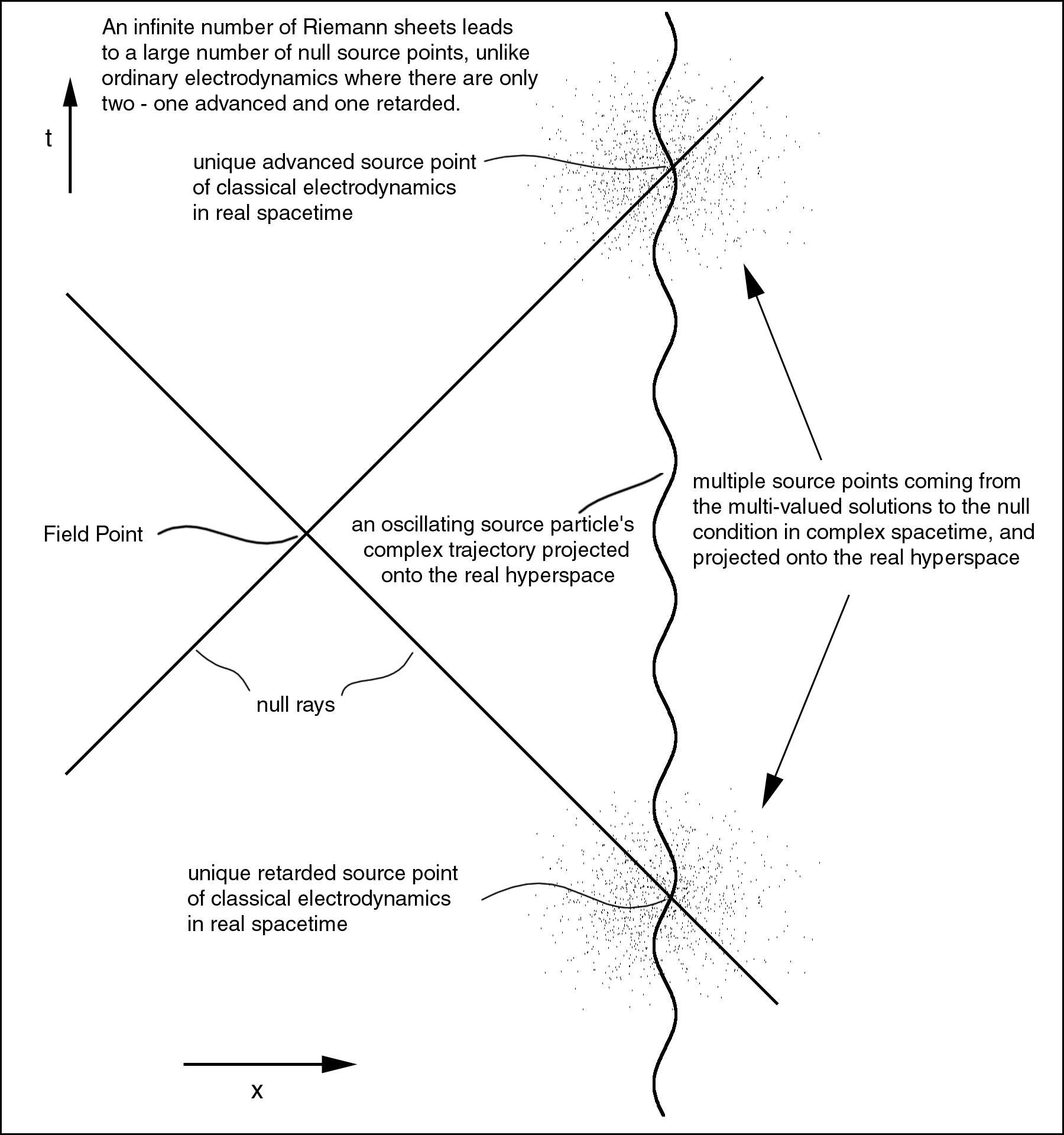
Figure 1: Qualitative illustration of multiple source points for Liénard-Wiechert potentials

7.2 Calculation of the roots in the asymptotic field limit

It is important to examine if these solutions radiate energy, which would render them unphysical. Even if they do radiate, however, it might be possible to find radiation backgrounds (such as the zero point radiation boyer_random_1975 ; de_la_pena_quantum_1996 ) with which these solutions could be in equilibrium, so that they would absorb as much energy on the average as they radiated, and leave the statistical distribution of radiation unchanged. In order to study the radiation from the source, we make the standard approximation for large $r=|\mathbf{x}|$, and let $t=x^{0}$. We assume that $\left|\mathbf{z}\right|\ll\left|\mathbf{x}\right|$ and therefore we make the standard far-field approximation with $x^{\mu}$ real

$$\left(x-z(s)\right)^{2}=0\thickapprox\left(t-z^{0}\right)^{2}-(\mathbf{x^{2}}\mathrm{-2}\mathbf{x}\cdot\mathbf{z})$$ (53)

$$t-z^{0}=t-\gamma s\thickapprox\pm(r-\hat{\mathbf{r}}\cdot\mathbf{z)}=\pm\left(r+\tau_{0}^{2}(\mathbf{a}_{s}(0)\cdot\mathbf{x})e^{-is/\tau_{0}}/r-\hat{\mathbf{r}}\cdot\mathbf{\Omega}\right)$$ (54)

For the retarded solution $s\uparrow$we choose the + sign and obtain

$$\gamma s\uparrow-(t-r+\hat{\mathbf{r}}\cdot\mathbf{\Omega})+\tau_{0}^{2}(\mathbf{a_{s}}(0)\cdot\mathbf{\hat{r}})e^{-is\uparrow/\tau_{0}}=0$$ (55)

$$A\equiv(t-r+\hat{\mathbf{r}}\cdot\mathbf{\Omega}),\>B\equiv\tau_{0}^{2}(\mathbf{a_{s}}(0)\cdot\mathbf{\hat{r}}),\>\gamma s\uparrow-A+Be^{-is\uparrow/\tau_{0}}=0$$ (56)

This equation can be solved for $s\uparrow$ again in terms of Lambert functions

$$s\uparrow=A/\gamma-i\tau_{0}W_{n}\left(-\frac{iBe^{-iA/\gamma\tau_{0}}}{\gamma\tau_{0}}\right),\>n\in\mathbb{Z}$$ (57)

$$s\uparrow_{n}=(t-r+\hat{\mathbf{r}}\cdot\mathbf{\Omega})/\gamma-i\tau_{0}W_{n}\left(-\frac{i\tau_{0}^{2}(\mathbf{a_{s}}(0)\cdot\mathbf{\hat{r}})e^{-i(t-r+\hat{\mathbf{r}}\cdot\mathbf{\Omega})/\gamma\tau_{0}}}{\gamma\tau_{0}}\right)$$ (58)

The solution for the advanced root $s\downarrow$ is

$$s\downarrow_{n}=(t+r-\hat{\mathbf{r}}\cdot\mathbf{\Omega})/\gamma-i\tau_{0}W_{n}\left(+\frac{i\tau_{0}^{2}(\mathbf{a_{s}}(0)\cdot\mathbf{\hat{r}})e^{-i(t+r-\hat{\mathbf{r}}\cdot\mathbf{\Omega})/\gamma\tau_{0}}}{\gamma\tau_{0}}\right)$$ (59)

The large argument behavior of the Lambert functions are given by the series expansion corless_lambert_1996

$$W_{k}(z) =log(z)+2\pi ik-log(log(z)+2\pi ik)$$

$$+\sum_{j=0}^{\infty}\sum_{m=1}^{\infty}c_{jm}log^{m}\left(log(z)+2\pi ik\right)\left(log(z)+2\pi ik\right)^{-j-m}$$ (60)

There are an infinite number of solutions as n is an arbitrary integer. The Poynting vector may be calculated from (3). The potential is then given by (40). The analytic structure of the multi-sheeted Lambert functions are of critical importance in understanding these solutions. We follow the branch-cut conventions of corless_lambert_1996 . $W_{0}(z)$ is special as it has a branch point at $-1/e$ with a cut $\{z:-\infty<z\leq-1/e\}$. $W_{1}(z)$ and $W_{-1}(z)$ each have two cuts given by $\{z:-\infty<z\leq-1/e\}$ and $\{z:-\infty<z\leq 0\}$. All other branches have a single cut $\{z:-\infty<z\leq 0\}$. The function $W_{k+1}$ is obtained from the function $W_{k}$ by analytically continuing it through its branch cut in the counterclockwise direction, mimicking the complex log function corless_lambert_1996 . Imagine holding $t$ and $\hat{\mathbf{r}}$ fixed, and analytically continuing the solutions by increasing $r$. Recall (21), so that there is an exponential factor in the argument of $W_{n}$ of the form

$$phase\>factor=e^{\pm i\varphi-i(t-r+\hat{\mathbf{r}}\cdot\mathbf{o})/\gamma\tau_{0}}$$ (61)

Every time its phase increases by $2\pi$, the Lambert function moves to a different branch. The asymptotic field, which determines whether or not the particle radiates, depends on how we take $r$ to $\infty.$ If we hold $\varphi$ fixed we get one result, if we hold $r/\gamma\tau_{0}\pm\varphi$ fixed we get another.

7.2.1 Holding $\left((r-t)/\gamma\tau_{0}\pm\varphi\right)$ fixed as $r\rightarrow\infty$

If we hold the phase (61) fixed as we take $r$ to $\infty$ then $n$ does not change with $r$ and the Lambert function stays on the same branch as we approach the $r\rightarrow\infty$ limit. In this case we have the result

$$s\uparrow_{n}=(t-r+\hat{\mathbf{r}}\cdot\mathbf{\Omega})/\gamma+O(1)$$ (62)

$$s\downarrow_{n}=(t+r-\hat{\mathbf{r}}\cdot\mathbf{\Omega})/\gamma+O(1)$$ (63)

This is reasonable behavior for an oscillating charge, and these solutions would lead to radiation.

7.2.2 Holding $\varphi$ and $t$ fixed as $r\rightarrow\infty$

This gives a different result for the asymptotic behavior. We have the following recursion relations for analytic continuations starting at $r$ and ending at $r+2\pi\gamma\tau_{0}$with $t$ and $\varphi$ held fixed

$$s\uparrow_{n}(r+2\pi\gamma\tau_{0})=s\uparrow_{n+1}(r)-2\pi\tau_{0},\;n\notin\left\{-1,0\right\}$$ (64)

$$s\downarrow_{n}(r+2\pi\gamma\tau_{0})=s\downarrow_{n-1}(r)+2\pi\tau_{0},\;n\notin\left\{0,1\right\}$$ (65)

When $n=-1,\,0,\,\mathrm{or}\,1$ the behavior depends on the magnitude of the argument of $W_{n}$. For example,

$$s\uparrow_{0}(r+2\pi\gamma\tau_{0})=s\uparrow_{0}(r)-2\pi\tau_{0},\;\mathrm{if}\>\left|\frac{\tau_{0}^{2}(\mathbf{a}(0)\cdot\mathbf{\hat{r}})}{\gamma\tau_{0}}\right|<1/e$$ (66)

$$s\uparrow_{-1}(r+2\pi\gamma\tau_{0})=s\uparrow_{1}(r)-2\pi\tau_{0},\;\mathrm{if}\>\left|\frac{\tau_{0}^{2}(\mathbf{a}(0)\cdot\mathbf{\hat{r}})}{\gamma\tau_{0}}\right|<1/e$$ (67)

and so in this case if the argument of $W_{n}$ is below the critical value of $1/e$ and the solution starts on the principal branch with $n=0$, it will stay on the principal branch for all $r$. In this case $z(s)$ is single-valued. Otherwise, as $r\rightarrow\infty,$the branch function $n(r)$ will approach infinity in a linear staircase fashion. In general $n(r)$ will be either fixed at $0$ or a step-like function of $r$ which grows linearly (expect for $n=-1$) in $r$ . If r is held fixed and $t$ varied, a similar behavior ensues in the variables $r-t$ for the retarded case and $r+t$ for the advanced case. In order to calculate the radiation, the asymptotic fields for large $r$ and fixed $t$ are required. The Lambert function satisfies the equation $z=W_{n}(z)e^{W_{n}(z)}$, and this is useful for asymptotic analysis. For large $n$ we have from (60)

$$W_{n}(\Gamma)=\left(log(\Gamma)+2\pi in\right)\>-log(log(\Gamma)+2\pi in)\>+o(log(n))$$ (68)

$$\Gamma\equiv\Lambda e^{-i(t-r+\hat{\mathbf{r}}\cdot\mathbf{o})/\gamma\tau_{0}},\;\Lambda\equiv-\frac{i\tau_{0}(\mathbf{a}(0)\cdot\mathbf{\hat{r}})}{\gamma}$$ (69)

$$s\uparrow_{n}=(t-r+\hat{\mathbf{r}}\cdot\mathbf{o})/\gamma-i\tau_{0}\left[(log(\Gamma)+2\pi in)-log(log(\Gamma)+2\pi in)\right]+o(log(n)))$$ (70)

but $n$ grows in a staircase fashion as $n\sim(r-t)/2\pi\gamma\tau_{0}+n_{0}$ if we analytically continue along a radial line, for some constant $n_{0}$, so

$$s\uparrow_{n}=i\tau_{0}log(r)+o(log(r))$$ (71)

This is perplexing behavior. Now consider the case where $n=0$ and the argument of $W_{0}$ is less in magnitude than the critical value of $1/e$. Let us perform a Taylor’s series expansion keeping only the first term $W_{0}(z)=z+o(z)$, for small $\left|z\right|$.

$$s\uparrow_{0}\approx(t-r+\hat{\mathbf{r}}\cdot\mathbf{o})/\gamma-\frac{\tau_{0}^{2}(\mathbf{a}(0)\cdot\mathbf{\hat{r}})e^{-i(t-r+\hat{\mathbf{r}}\cdot\mathbf{o})/\gamma\tau_{0}}}{\gamma}$$ (72)

This solution will radiate energy away, but the solution stays on the same Riemann sheet as we take the limit. So we have an infinite number of Riemann sheets for the solutions. Another example of multiple sheet structure in the literature occurs when there are multiple K-N particles presentburinskii_wonderful_2005 .

8 Suppressing of radiation and magnetic currents with weighting factors that are functions of x

When the previous results for the retarded proper times are used to calculate the asymptotic fields, the author believes based on extensive analysis that the system will either radiate electromagnetic energy or else have some other unphysical feature. Moreover, and more disturbingly, the asymptotic field depends on the path of analytic continuation to large $r$. Adding together even an infinite number of roots with complex weighting constants does not seem to alter this conclusion. In order to suppress the radiation, we therefore consider allowing the weighting factors $w_{i}$ in (40) to be functions of the field point $x$. So long as these functions are analytic (or at least holomorphic) in the coordinates, the resulting fields will be too. It is convenient to rewrite (40) using (18) as follows

$$A^{\mu}(x)=A_{Coul}^{\mu}(x)+A_{Rad}^{\mu}(x)$$ (73)

$$A_{Coul}^{\mu}(x)=\sum_{j=1}^{N}w_{j}(x)\frac{q\gamma\delta_{0}^{\mu}}{v(s_{j}(x))\cdot(x-z(s_{j}(x)))},\>\sum_{j=1}^{N}w_{j}(x)=1$$ (74)

$$A_{Rad}^{\mu}(x)=\sum_{j=1}^{N}w_{j}(x)\frac{qi\tau_{0}e^{-is_{j}(x)/\tau_{0}}a_{\pm}^{\mu}(0)}{v(s_{j}(x))\cdot(x-z(s_{j}(x)))}$$ (75)

and where $s_{j}(x)$ are the proper-time null roots. The potential $A_{Coul}$ determines the Coulomb field and the potential $A_{Rad}$ determines the radiation field. In order to calculate the radiation field, we must perform the following steps following our procedure $W^{\mu\nu}(x)=\partial^{[\mu}A^{\nu]}+i(*\partial^{[\mu}A^{\nu]})$, where the real part of $W$ gives the physical Faraday tensor. Note the important fact that

$$*\partial^{[\mu}A^{\nu]}=i\partial^{[\mu}A^{\nu]}\Rightarrow W^{\mu\nu}(x)=0$$ (76)

In other words, if $\partial^{[\mu}A^{\nu]}$ is self-dual, then the resulting $W$ field is zero. In order for there to be radiation from a current source, the fields produced must fall to zero as $1/r$ for large $r$. Consequently, the only term that can contribute radiation is $A_{Rad}$. Note that $A_{Rad}$ has the simple form of a scalar function of $x$ times a constant 4-vector $a_{\pm}^{\mu}(0)$. We have for large $r$, $\partial^{[\mu}A^{\nu]}=\partial^{[\mu}A_{Rad}^{\nu]}+o(\frac{1}{r})$. If the $A_{Rad}$ happens to be self-dual, then there will be no radiation. But the $w_{j}(x)$ are now assumed to be arbitrary functions, and we can choose them such that this is the case. The following potential functions are self dual in this sense

$$A_{SD}(x)=f_{\pm}(x^{3}\mp x^{0},x^{1}\pm ix^{2})a_{\pm}(0)$$ (77)

where $f_{\pm}$ are arbitrary holomorphic functions of their arguments. So to cloak radiation for + or - chirality, we must choose the weighting functions to satisfy

$$\sum_{j=1}^{N}w_{j}(x)\frac{qi\tau_{0}e^{-is_{j}(x)/\tau_{0}}}{v(s_{j}(x))\cdot(x-z(s_{j}(x)))}=f_{\pm}(x^{3}\mp x^{0},x^{1}\pm ix^{2});\quad\sum_{j=1}^{N}w_{j}(x)=1$$ (78)

Since two equations must be satisfied, at least two roots must be included in the solution. Denote two such roots by index 1 and 2. The equations can be solved simply with the result

$$\left(\begin{array}[]{c}w_{1}\\ w_{2}\end{array}\right)=\frac{1}{C_{1}-C_{2}}\left(\begin{array}[]{c}f_{\pm}-C_{2}\\ -f_{\pm}+C_{1}\end{array}\right)$$ (79)

where the two $C$ values in this formula are the functions multiplying the respective weight functions $w$ in (78). To this solution might be added by superposition any combination of the weighting functions which satisfy the associated homogeneous equations. Thus, there are a large number of non-radiating solutions. When the cloaking conditions are satisfied, we can write

$$W^{\mu\nu}=\partial^{[\mu}A_{Coul}^{\nu]}+i(*\partial^{[\mu}A_{Coul}^{\nu]})$$ (80)

and the radiation term vanishes. The weighting functions may be multi-sheeted too. The resulting “cloaked” field will still generally be multi-sheeted, except in the far-field where it will be just the single-valued Coulomb field. The near field will contain electromagnetic currents which depend on the weighting functions, and will not be sourceless in general.

We can eliminate magnetic currents by again exploiting position dependent weighting functions. In the compact notation of exterior derivatives and differential forms (in 4 dimensions), the absence of magnetic 4-current on the real hyperspace requires that $d(ReW)=0$, the electromagnetic Bianchi identity. This expression is linear in the weighting functions $w_{i}$ and their first derivatives. In order to solve it, four additional weighted root terms would be required in general, because the dual of this equation is the magnetic current 1-form which has four independent components. The solution is more complicated than the suppression of radiation, since it involves derivatives of the weighting functions, but it is linear and first order, and there should be solutions. In general relativity, the most studied electromagnetic systems are sourceless ones. We can also generate these by instead imposing the conditions $dW=0$.

Surprisingly, with only three roots one can enforce that the fields of the oscillating particle in real space-time are exactly the same as the static K-N solution. This can be achieved by adding an additional contraint equation for the vector potential 1-forms $A_{coul}=A_{Kerr-Newman}$ which is linear in the weighting functions, but does not involve any derivatives, and so only a single extra root is required (because the vector potentials have only one nonzero component). This is possible because both terms have the same asymptotic behavior for large r. This solution of course does not have any magnetic currents, and in fact it is sourceless. This suggests that such solutions do exist. Given this, a perturbative approach to study small deviations about the K-N solution might be interesting. It also shows that stringlike singularities can appear in this theory too.

The K_N solution has infinite electrostatic energy, but there may exist other finite energy solutions for the fields here, perhaps involving still more roots, which may even be single valued, but have a more complex near-field structure.

One question that naturally arises is what is the state of minimum electrostatic energy? This will depend on the number of roots included in the sum, assuming that there are some solutions for which the energy is not infinite. Relevant to the question of emergence, the quantum mechanical wave equations for free particles are closely related to non-radiating electromagnetic sources davidson_quantum_2007 .

9 Electromagnetic self energy and field singularities

The electromagnetic field energy will be infinite if the complex vector potential has a singularity. One way a singularity can occur is if the denominator of any of the terms in the sum (37) vanish which requires simultaneously

$$\left(x-z(s)\right)^{2}=0,\>\mathrm{and}\>\frac{\partial}{\partial s}\left(x-z(s)\right)^{2}=0$$ (81)

and which for the present case becomes (together with (39))

$$2s-(C_{A}+C_{R})=\frac{-i}{\tau_{0}}De^{-is/\tau_{0}}$$ (82)

This equation can be solved for $s$ again with Lambert functions

$$s=\frac{1}{2}\left[\left(C_{A}+C_{R}\right)-2i\tau_{0}W_{n}\left(\frac{De^{-i\left(C_{A}+C_{R}\right)/2\tau_{0}}}{2\tau_{0}^{2}}\right)\right]$$ (83)

From dividing (45) and (82) we get a quadratic equation

$$2\left(s-\frac{\left(C_{A}+C_{R}\right)}{2}\right)+\frac{i}{\tau_{0}}\left(\left(s-\frac{\left(C_{A}+C_{R}\right)}{2}\right)^{2}-\left(\frac{C_{A}-C_{R}}{2}\right)^{2}\right)=0$$ (84)

and these two equations must be simultaneously satisfied, and solving this problem is very difficult. If the singularity occurs on the physical Riemann sheet, the electromagnetic self energy will be infinite. However, if all the singularities are off the physically realized Riemann sheets, then this energy could be finite. It is an open problem to elucidate the cases and calculate the self energies if any are finite. A particularly simple case occurs when $(\mathbf{x}-\mathbf{\mathbf{\Omega}})^{2}=0$ for then $C_{A}=C_{R}=x^{0}/\gamma=C$. This is the condition for points lying on the singularity ring of the static K-N particle, and then the equations simplify to

$$s=C+2i\tau_{0}=C-2i\tau_{0}W_{n}\left(\pm\frac{i}{2\tau_{0}}\sqrt{\frac{D}{e^{iC/\tau_{0}}}}\right)$$ (85)

so in order to have this singularity on this K-N ring, we must have $W_{n}\left(\pm\frac{i}{2\tau_{0}}\sqrt{\frac{D}{e^{iC/\tau_{0}}}}\right)=-1$. The only solutions to $W_{n}(y)=-1$ are $y=-1/e$, $n=0,1.$ There is always some azimuthal angle $\varphi$ that gives the right phase to the argument of $W_{n}$ by giving the phase of $D$ from (48) the correct value. Then magnitude of $D$ is determined uniquely if this singularity is to occur. For the elementary particle values, this magnitude value is not satisfied, and therefore there are no field singularities on the K-N ring. There might be singularities at other field points though, and perhaps there might even be singularities along string-like curves in space. It seems possible that there could be root solutions that don’t have any field singularities on the physical sheet too.

10 Motion with weak external forces applied

In an external electromagnetic field, we take the equation of motion to be

$$m\frac{d^{2}z}{ds^{2}}^{\mu}=qF_{ext}^{\mu\nu}\frac{dz_{\upsilon}}{ds}+im\tau_{0}\left(\frac{d^{3}z}{ds^{3}}^{\mu}-\left(\frac{d^{2}z}{ds^{2}}\right)^{2}\frac{dz}{ds}^{\mu}\right)$$ (86)

The external Faraday tensor $F_{ext}$ here is real on the real hyperspace, but is generally complex in the rest of the complex space-time by analytic continuation. We assume that the fields are weak and slowly varying on the time scale of $\tau_{0}.$ This reduces to simply the Lorentz equation if we ignore the Schott and radiation terms, which now have a factor of $i$ in front of them. This factor is rather mysterious, and it seems questionable. The equation gives results that we actually observe in nature, at least qualitatively, and it is much better than the ordinary LDE equation in this regard, so we will persist with this line of reasoning, even though the strange form of the equation raises a number of questions and must be considered preliminary. Consider the simplified case where we ignore the radiation term. The equation then becomes

$$m\frac{d^{2}z}{ds^{2}}^{\mu}=qF_{ext\,\nu}^{\mu}\frac{dz^{\nu}}{ds}+im\tau_{0}\frac{d^{3}z}{ds^{3}}^{\mu}$$ (87)

In this formula, the mass $m$ is the observed mass divided by $\gamma$. It is natural to make a guiding center approximation to this. The particle moves in a tight high-frequency oscillation perturbed by the weak field. One finds quite generally that the Riemann structure of the solution is a distortion of the Riemann structure of the simpler pure zitterbewegung case described above. Thus, in the guiding center approximation there will generally be an infinite number of retarded time points, and the cloaking mechanism for shielding radiation can be used for these too. Therefore, the radiation can be greatly suppressed and in some cases even made zero.

10.1 Motion in a 3D harmonic oscillator central force

$$m\frac{d^{2}z}{ds^{2}}^{j}=-kz^{j}+im\tau_{0}\left(\frac{d^{3}z}{ds^{3}}^{j}-\left(\frac{d^{2}z}{ds^{2}}\right)^{2}\frac{dz}{ds}^{j}\right),\>j=1,2,3$$ (88)

There will be exact solutions with $a\cdot a=0$ as follows. Then the equation has solutions of the form $\mathbf{\mathrm{z\mathrm{{}^{j}(s)=}z^{j}(0)e^{i\omega s}}}$ with $\mathbf{z(0)\cdot z(0)}=0$. We can take $\mathrm{\mathbf{z}}\mathbf{(0)}$ to be proportional to either of the null vectors $\mathbf{a_{\pm}(0)}$ 3-vectors for example for some arbitrary spin axis. Then the frequency equation becomes $\tau_{0}\omega^{3}+\omega^{2}-k/m=0$. There are three roots to this which are approximately $\omega=\pm\sqrt{k/m},-1/\tau_{0}$. A class of exact solutions are given by a linear superposition of these

$$\mathbf{z(s)}=\mathbf{a_{\pm}(0)}\sum_{j=1}^{3}c_{j}e^{i\omega_{j}s},\>\mathrm{and}\>z^{0}(s)=\gamma s$$ (89)

for arbitrary complex constants $c_{j}$. These solutions are more complicated than the single-frequency zitterbewegung solutions. Nevertheless, we expect that they will certainly have multiple null roots for the radiation calculation. Therefore, the same cloaking technique that was proposed to eliminate radiation in the zitterbewegung case can be applied in the present circumstance to reduce or eliminate the radiation from these harmonic oscillator solutions as well.

11 Particle morphology and complementarity

We have seen that even if we take the interpretation that the motion of the solution to the Lorentz-Dirac equation in complex space-time is a one dimensional curve, as ordinary classical mechanics would suggest, we still find that the source points in the Liénard-Wiechert potentials are not lying on this same curve, and in fact they are distributed on a subset of the space-time world sheet of a string as in Burinskii burinskii_gravitational_2011 . The static K-N solution has a string-like ring singularity. In the present case, the locus of singular points might also be string-like, but it is difficult to show this because it requires solutions to the null root equation for field points which are in the near-field of the particle. For a singularity to occur, additional conditions must be satisfied as in section 9 above. The set of field singularities may still lie on a string, but this is not obvious to the author at least. One cannot prove this without detailed numerical calculations or perhaps with clever analytical methods. Moreover, as we are considering superpositions of multiple roots, the solution might involve more than one string. So even if we try and treat the motion as if it were one-dimensional in the complex space-time, we are likely forced into a string-like picture for the source points of the field, and possibly for the singularities of the field as well.

Complex space-time is an eight dimensional manifold. Imagine that all the particles of the universe each have a string-like world sheet in this manifold. Imagine too a kind of Mach’s principle for this space, namely, that given any clump of matter consisting of large numbers of such particles, that the averaged coordinate values of all this matter are narrowly clustered around a 4-dimensional real hyperspace, and that this hyperspace has been singled out from all others by this fact - a spontaneous symmetry breaking. This is our world of Minkowski space. Then objects consisting of large numbers of such particles can be described by real-valued positions and times. This elevates the projection to real values of the complex coordinates of individual particles to a distinguished meaning when being observed by macroscopic experimental apparatus.

The duality between pointlike and string-like behavior is similar in spirit to Bohr’s complementarity philosophy for quantum phenomena, although we are considering a purely classical field theory here, and it’s also very suggestive from the point of view of emergent quantum mechanics. Just as quantum mechanics presents us with paradoxical complentarity, so too the present theory seems to do the same.

12 Conclusion

The picture that emerges from this model is of a particle with a peculiar internal oscillation, and whose electromagnetic fields are dependent on a set of complex weighting functions. The theory eliminates runaway solutions from classical electromagnetism and replaces them with oscillating solutions that look similar to zitterbewegung. These solutions oscillate in time, which gives a tangible model for the de Broglie clock. They allow a cloaking mechanism for radiationless accelerated motion, both in the self-oscillating free particle case and the central harmonic force case. Some might have string-like singularities, or even have finite electromagnetic energy. The non-uniqueness is vaguely similar to wave-particle duality.

The calculation of the gravitational metric along the lines of debney_solutions_1969 ; burinskii_nonstationary_1995 is an extremely important task needed to build confidence and add value to the ideas presented here.

- (1) Adamo, T.M., Kozameh, C., Newman, E.T.: Null geodesic congruences, Asymptotically-Flat spacetimes and their physical interpretation. Living Reviews in Relativity (www.livingreviews.org/lrr-2009-6) 12(6) (2009)
- (2) Adler, S.L.: Quantum theory as an emergent phenomenon: the statistical mechanics of matrix models as the precursor of quantum field theory. Cambridge University Press (2004)
- (3) Ali, S.T., Gagnon, R., Prugovecki, E.: Conserved quantum probability currents on stochastic phase space. Can. J. Phys. 59(6), 807–811 (1981)
- (4) Barut, A.O., Bracken, A.J.: Zitterbewegung and the internal geometry of the electron. Phys. Rev. D 23(10), 2454 (1981)
- (5) Bjorken, J.D., Drell, S.D.: Relativistic Quantum Mechanics, 1 edn. McGraw-Hill (1998)
- (6) Boyer, T.H.: Random electrodynamics: The theory of classical electrodynamics with classical electromagnetic zero-point radiation. Phys. Rev. D 11, 790–808 (1975)
- (7) de Broglie, L.: Researches sur la théorie des quanta, P.H. d. thesis, english translation. Ph.D. thesis, University of Paris (1924)
- (8) Browne, P.: Electron spin and radiative reaction. Ann. Phys. 59, 254–258 (1970)
- (9) Burinskii, A.: Wonderful consequences of the kerr theorem. arXiv:hep-th/0506006 (2005)
- (10) Burinskii, A.: Kerr geometry as Space-Time structure of the dirac electron. arxiv.org 0712.0577 (2007)
- (11) Burinskii, A.: The dirac – Kerr-Newman electron. Gravit. Cosmol. 14, 109–122 (2008)
- (12) Burinskii, A.: Regularized Kerr-Newman solution as a gravitating soliton. arXiv:1003.2928 (2010)
- (13) Burinskii, A.: Gravitational strings beyond quantum theory: Electron as a closed string. arXiv:1109.3872 (2011)
- (14) Burinskii, A., Kerr, R.P.: Nonstationary kerr congruences. arXiv:gr-qc/9501012 (1995)
- (15) Calvani, M., Stuchlík, Z.: The latitudinal motion of test particles in the Kerr-Newman dyon space-time. Il Nuovo Cimento B 70(1), 128–140 (1982)
- (16) Carroll, R.: Gravity and the quantum potential. gr-qc/0406004 (2004)
- (17) Carter, B.: Global structure of the kerr family of gravitational fields. Phys. Rev. 174(5), 1559 (1968)
- (18) Corless, R.M., Gonnet, G.H., Hare, D.E.G., Jerey, D.J., Knuth, D.E.: On the lambert w function. Adv. Comput. Math. 5, 329—359 (1996)
- (19) Davidson, M.: The quark-gluon plasma, turbulence, and quantum mechanics. arxiv.org 0807.1990 (2008)
- (20) Davidson, M.: The quark-gluon plasma and the stochastic interpretation of quantum mechanics. Physica E: Low-dimensional Systems and Nanostructures 42(3), 317–322 (2010)
- (21) Davidson, M.P.: Quantum wave equations and non-radiating electromagnetic sources. Ann. Phys. 322(9), 2195–2210 (2007)
- (22) Debney, G.C., Kerr, R.P., Schild, A.: Solutions of the einstein and Einstein-Maxwell equations. J. Math. Phys. 10(10), 1842–1854 (1969)
- (23) Dirac, P.A.M.: Classical theory of radiating electrons. Proceedings of the Royal Society of London. Series A, Mathematical and Physical Sciences 167(929), 148–169 (1938)
- (24) Dirac, P.A.M.: The principles of quantum mechanics. Clarendon Press (1978)
- (25) Guoanere, M., Spighel, M., Cue, N., Gaillard, M.J., Genre, R., Kirsch, R., Poizat, J.C., Remillieux, J., Catillon, P., Roussel, L.: Experimental observation compatible with the particle internal clock in a channeling experiment. Annales de la Fondation Louis de Broglie 33(1-2), 85–91 (2008)
- (26) Hestenes, D.: The zitterbewegung interpretation of quantum mechanics. Found. Phys. 20, 1213–1232 (1990)
- (27) ’t Hooft, G.: Equivalence relations between deterministic and quantum mechanical systems. J. Stat. Phys. 53(1-2), 323–344 (1988)
- (28) ’t Hooft, G.: Determinism and dissipation in quantum gravity, erice lecture. arxiv.org hep-th/0003005 (2000)
- (29) ’t Hooft, G.: How does god play dice? (Pre-)Determinism at the planck scale. arxiv.org hep-th/0104219 (2001)
- (30) ’t Hooft, G.: Determinism beneath quantum mechanics. In: A.C. Elitzur, S. Dolev, N. Kolenda (eds.) Quo Vadis Quantum Mechanics?, The Frontiers Collection, p. 99–111. Springer-Verlag, Berlin/Heidelberg (2005)
- (31) ’t Hooft, G.: Entangled quantum states in a local deterministic theory. arxiv.org 0908.3408 (2009)
- (32) Huang, K.: On the zitterbewegung of the dirac electron. Am. J. Phys. 20(8), 479–484 (1952)
- (33) Jackson, J.D.: Classical electrodynamics, 3rd Ed. Wiley (1999)
- (34) Jackson, J.D.: Comment on preacceleration without radiation. Am. J. Phys. 75(9), 844 (2007)
- (35) Kasuya, M.: Exact solution of a rotating dyon black hole. Phys. Rev. D 25(4), 995 (1982)
- (36) Landau, L.D., Lifshitz, E.M.: The classical theory of fields. Addison-Wesley, Cambridge, MA (1951)
- (37) Lynden-Bell, D.: A magic electromagnetic field. In: Stellar Astrophys. Fluid Dyn., p. 369–375 (2003)
- (38) Lynden-Bell, D.: Electromagnetic magic: The relativistically rotating disk. Phys. Rev. D 70(10), 105,017 (2004)
- (39) Markopoulou, F., Smolin, L.: Quantum theory from quantum gravity. Phys. Rev. D 70(12), 124,029 (2004)
- (40) Morris, M., Thorne, K., Yurtsever, U.: Wormholes, time machines, and the weak energy condition. Phys. Rev. Lett. 61(13), 1446–1449 (1988)
- (41) Morris, M.S.: Wormholes in spacetime and their use for interstellar travel: A tool for teaching general relativity. Am. J. Phys. 56(5), 395 (1988)
- (42) Newman, E.T.: Complex coordinate transformations and the Schwarzschild-Kerr metrics. J. Math. Phys. 14, 774 (1973)
- (43) Newman, E.T.: Maxwell’s equations and complex minkowski space. J. Math. Phys. 14(1), 102 (1973)
- (44) Newman, E.T.: Heaven and its properties. Gen. Relativ. Gravit. 7(1), 107–111 (1976)
- (45) Newman, E.T.: Classical, geometric origin of magnetic moments, spin-angular momentum, and the dirac gyromagnetic ratio. Phys. Rev. D 65(10), 104,005 (2002)
- (46) Newman, E.T., Couch, E., Chinnapared, K., Exton, A., Prakash, A., Torrence, R.: Metric of a rotating, charged mass. J. Math. Phys. 6(6), 918 (1965)
- (47) Newton, T.D., Wigner, E.P.: Localized states for elementary systems. Rev. Mod. Phys. 21(3), 400–406 (1949)
- (48) de la Peña, L., Cetto, A.M.: The quantum dice : an introduction to stochastic electrodynamics. Kluwer Academic Publishers, Dordrecht ;;Boston (1996)
- (49) Pekeris, C.L., Frankowski, K.: The electromagnetic field of a Kerr-Newman source. Phys. Rev. A 36(11), 5118 (1987)
- (50) Penrose, R.: The question of cosmic censorship. J. Astrophys. Astron. 20(3-4), 233–248 (1999)
- (51) Plass, G.N.: Classical electrodynamic equations of motion with radiative reaction. Rev. Mod. Phys. 33(1), 37 (1961)
- (52) Prugovecki, E.: Consistent formulation of relativistic dynamics for massive spin-zero particles in external fields. Phys. Rev. D 18(10), 3655–3675 (1978)
- (53) Prugovecki, E.: Stochastic Quantum Mechanics and Quantum Spacetime: Consistent Unification of Relativity and Quantum Theory Based on Stochastic Spaces. Springer (1984)
- (54) Ringermacher, H.I.: Intrinsic geometry of curves and the minkowski force. Phys. Lett. A 74(6), 381–383 (1979)
- (55) Rohrlich, F.: Classical charged particles. World Scientific (2007)
- (56) Schroeck, F.: Quantum mechanics on phase space. Kluwer Academic (1996)
- (57) Schroedinger, E.: Über die kräftefreie bewegung in der relativistischen quantenmechanik. Sitzungsberichte der Preussischen Akademie der Wissenschaften. Physikalisch-mathematische Klasse 24, 418–428 (1930)
- (58) Scott, T.C., Mann, R., Martinez II, R.E.: General relativity and quantum mechanics: towards a generalization of the lambert w function a generalization of the lambert w function. Appl. Algebra Eng., Commun. Comput. 17(1), 41–47 (2006)
- (59) Sidharth, B.G.: Revisiting zitterbewegung. Int. J. Theor. Phy. 48(2), 497–506 (2008)
- (60) Streater, R.F., Wightman, A.S.: PCT, spin and statistics, and all that. Princeton University Press (2000)
- (61) Teitelboim, C.: Splitting of the maxwell tensor: Radiation reaction without advanced fields. Phys. Rev. D 1(6), 1572 (1970)
- (62) Teitelboim, C., Villarroel, D., Weert, C.G.: Classical electrodynamics of retarded fields and point particles. La Rivista del Nuovo Cimento 3(9), 1–64 (1980)
- (63) Weinberg, S.: Collapse of the state vector. arXiv:1109.6462 (2011)
- (64) Wheeler, J.A., Feynman, R.P.: Interaction with the absorber as the mechanism of radiation. Rev. Mod. Phys. 17(2-3), 157 (1945)
- (65) Wightman, A.S.: On the localizability of quantum mechanical systems. Rev. Mod. Phys. 34(4), 845–872 (1962)