Inapproximability of Treewidth,
One-Shot Pebbling, and Related Layout Problems

We study the approximability of a number of graph problems: treewidth and pathwidth of graphs, one-shot black (and black-white) pebbling costs of directed acyclic graphs, and a variety of different graph layout problems such as minimum cut linear arrangement and interval graph completion. We show that, assuming the recently introduced Small Set Expansion Conjecture, all of these problems are hard to approximate within any constant factor.

1 Introduction

One of the great accomplishments in the last twenty years in complexity theory has been the development of ideas that has led to a deep understanding of the approximability of an astonishing number of NP-hard optimization problems. More recently, in the last ten years, the formulation of the Unique Games Conjecture (UGC) due to Khot [Kho02] has inspired a remarkable body of work, clarifying the complexity of many optimization problems, and exposing the central role of semidefinite programming in the development of approximation algorithms.

Despite this tremendous progress, for certain expansion problems such as the $c$-Balanced Separator problem, and graph layout problems such as the Minimum Linear Arrangement (MLA) problem, their approximation status remained unresolved. That is, even assuming the UGC is not known to be sufficient to obtain hardness of approximation for either of these problems. Moreover, the approximability of many other graph layout problems is similarly unresolved, even under the UGC. Intuitively this is because the hard instances for these problems seem to require a certain global structure such as expansion. Typical reductions for these problems are gadget reductions which preserve global properties of the unique games instance, such as the lack of expansion. Therefore, barring radically new types of reductions that do not preserve global properties, proving hardness for $c$-Balanced Separator seems to require a stronger version of UGC, where the instance is guaranteed to have good expansion.

In [RS10], the Small Set Expansion (SSE) Conjecture was introduced, and it was shown that it implies the UGC, and that the SSE Conjecture follows if one assumes that the UGC is true for somewhat expanding graphs. In follow-up work by Raghavendra et al. [RST10], it was shown that the SSE Conjecture is in fact equivalent to the UGC on somewhat expanding graphs, and that the SSE Conjecture implies hardness of approximation for $c$-Balanced Separator and MLA. In this light, the Small Set Expansion conjecture serves as a natural unified conjecture that yields all of the implications of UGC and also hardness for expansion-like problems that appear to be beyond the reach of the UGC.

In this paper, we study the approximability of a host of such graph layout problems, including: treewidth and pathwidth of graphs, one-shot black and black-white pebbling, Minimum Cut Linear Arrangement (MCLA) and Interval Graph Completion (IGC). We prove that all of these problems are SSE-hard to approximate to within any constant factor. Our main contributions, giving SSE-hardness of approximation for all of the graph layout problems mentioned above, are described in the following subsections. For all of these problems, no evidence of hardness of approximation was known prior to our results.

It should be noted that the status of the SSE Conjecture is very open at this point. In particular, by the recent result of Arora et al. [ABS10] (see also subsequent work [BRS11, GS11]), it has algorithms running in subexponential time. Still, despite this recent progress providing negative evidence against the SSE Conjecture, it remains open, and we think that investigating what open problems in approximability we can show SSE-hardness for is a worthwhile venture.

1.1 Width Parameters of Graphs

The treewidth of a graph, introduced by Robertson and Seymour [RS84, RS86], is a fundamental parameter of a graph that measures how close a graph is to being a tree. The concept is very important since problems of small treewidth can usually be solved efficiently by dynamic programming. Indeed, a large body of NP-hard problems (including all problems definable in monadic second-order logic [Cou90]) are solvable in polynomial time and often even linear time on graphs of bounded treewidth. Examples of such optimization problems include finding the maximum independent set in a graph, as well as finding Hamiltonian cycles. In machine learning, tree decompositions play a key role in the development of efficient algorithms for fundamental problems such as probabilistic inference, constraint satisfaction and query optimization. (See the excellent survey [Bod05] for motivation, including theoretical as well as practical applications of treewidth.)

The complexity of approximating treewidth is a longstanding open problem. Determining the exact treewidth of a graph and producing an associated optimal tree decomposition (see Definition 2.4) is known to be NP-hard [ACP87]. A central open problem is to determine whether or not there exists a polynomial time constant factor approximation algorithm for treewidth (see e.g., [BGHK95, FHL05, Bod05]). The current best polynomial time approximation algortihm for treewidth [FHL05], computes the treewidth $\operatorname{\sf{tw}}(G)$ within a factor $O(\sqrt{\log\operatorname{\sf{tw}}(G)})$. On the other hand, the only hardness result to date for treewidth shows that it is NP-hard to compute treewidth within an additive error of $n^{\epsilon}$ for some $\epsilon>0$ [BGHK95]. No hardness of approximation is known and not even the possibility of a polynomial-time approximation scheme for treewidth has been ruled out. In many important special classes of graphs, such as planar graphs [ST94], asteroidal triple-free graphs [BT03], and $H$-minor-free graphs [FHL05], constant factor approximations are known, but the general case has remained elusive.

On the positive side, there is a large body of literature developing fixed-parameter algorithms for treewidth. In particular, when the runtime is allowed to be exponential in the $\operatorname{\sf{tw}}(G)$ there are constant factor approximations. Furthermore, even exactly determining the treewidth is fixed-parameter tractable: there is a linear time algorithm for computing the (exact) treewidth for graphs of constant treewidth [Bod96].

A related graph parameter is the so-called pathwidth, which can be viewed as measuring how close $G$ is to a path. The pathwidth $\operatorname{\sf{pw}}(G)$ is always at least $\operatorname{\sf{tw}}(G)$, but can be much larger. The current state of affairs here is similar as for treewidth; though the current best approximation algorithm only has an approximation ratio of $O(\sqrt{\log\operatorname{\sf{pw}}(G)}\log n)$ [FHL05], the best hardness result is NP-hardness of additive $n^{\epsilon}$ error approximation.

Using the recently proposed Small Set Expansion (SSE) Conjecture [RS10] discussed earlier, we show that both $\operatorname{\sf{tw}}(G)$ and $\operatorname{\sf{pw}}(G)$ are hard to approximate within any constant factor. In fact, we show something stronger: it is hard to distinguish graphs with small pathwidth from graphs with large treewidth. Specifically:

Theorem 1.1.

For every $\alpha>1$ there is a $c>0$ such that given a graph $G=(V,E)$ it is SSE-hard to distinguish between the case when $\operatorname{\sf{pw}}(G)\leq c\cdot|V|$ and the case when $\operatorname{\sf{tw}}(G)\geq\alpha\cdot c\cdot|V|$.

In particular, both treewidth and pathwidth are SSE-hard to approximate within any constant factor.

This is the first result giving hardness of (relative) approximation for these problems, and gives evidence that no constant factor approximation algorithm exists for either of them.

1.2 Pebbling Problems

Graph pebbling is a rich and relatively mature topic in theoretical computer science. Pebbling is a game defined on a directed acyclic graph (DAG), where the goal is to pebble the sink nodes of the DAG according to certain rules, using the minimum number of pebbles. The rules for pebbling are as follows. A black pebble can be placed on a node if all of the node’s immediate predecessors contain pebbles, and can always be removed. A white pebble can always be placed on a node, but can only be removed if all of the node’s immediate predecessors contain pebbles. A pebbling strategy is a process of pebbling the sink nodes in a graph according to the above rules. The pebbling cost of a pebbling strategy is the maximum number of pebbles used in the strategy. The black-white pebbling cost of a DAG is the minimum pebbling cost of all possible pebbling strategies. The black pebbling cost is the minimum pebbling cost over all pebbling strategies that only use black pebbles.

Pebbling games were originally devised for studying programming languages and compiler construction, but have later found a broad range of applications in computational complexity theory. Pebbling is a tool for studying the relationship between computation time and space by means of a game played on directed acyclic graphs. It was employed to model register allocation, and to analyze the relative power of time and space as Turing machine resources. For a comprehensive recent survey on graph pebbling, see [Nor10].

Apart from the cost of a pebbling, another important measure is the pebbling time, which is the number of steps (pebble placements/removals) performed. In the context of measuring memory used by computations, this corresponds to computation time, and hence keeping the pebbling time small is a natural priority. The extreme case of this is what we refer to as one-shot pebbling, also known as progressive pebbling, considered in e.g. [Set73, Len81, KP86]. In one-shot pebbling, we have the restriction that each node can receive a pebble only once. Note that this restriction can cause a huge increase in the pebbling cost of the graph [LT82]. One-shot pebbling is also equivalent to a problem known as Register Sufficiency [RAK91].

The one-shot pebbling problem is easier to analyze for the following reasons. In the original pebbling problem, in order to achieve the minimum pebbling number, the pebbling time might be required to be exponentially long, which becomes impractical when $n$ is large. On the other hand, the one-shot pebbling problem is more amenable to complexity theoretic analysis as it minimizes the space used in a computation subject to the execution time being minimum. In particular, the decision problem for one-shot pebbling is in NP (whereas the unrestricted pebbling problems are PSPACE-complete).

The one-shot black pebbling problem and one-shot black-white pebbling problems admit an $O(\sqrt{\log n}\log n)$ approximation ratio. We show that they are SSE-hard to approximate to within any constant factor. For black pebbling we show that this holds for single sink DAGs with in-degree $2$, which is the canonical setting for pebbling games (it seems plausible that the black-white hardness can be shown to hold for this case as well, though we have not attempted to prove this).

Theorem 1.2.

It is SSE-hard to approximate the one-shot black pebbling problem within any constant factor, even in DAGs with a single sink and maximum in-degree $2$.

Theorem 1.3.

It is SSE-hard to approximate the one-shot black-white pebbling problem within any constant factor.

No hardness of approximation result of any form was known for one-shot pebbling problems. We believe that these results can be extended to obtain hardness for more relaxed versions of bounded time pebbling costs as well. We are currently working on this, and have some preliminary results.

1.3 The Connection: Layout Problems

The graph width and one-shot pebbling problems discussed in the previous sections may at first glance appear to be unrelated. However, both sets of problems are instances of a general family of problems, known as graph layout problems. In a graph layout problem (also known as an arrangement problem, or a vertex ordering problem), the goal is to find an ordering of the vertices, optimizing some condition on the edges, such as adjacent pairs being close. Layout problems are an important class of problems that have applications in many areas such as VLSI circuit design.

A classic example is the Minimum Cut Linear Arrangement Problem (MCLA). In this problem, the objective is to find a permutation $\pi$ of the vertices $V$ of an undirected graph $G=(V,E)$, such that the largest number of edges crossing any point,

$$\max_{i}|\{(u,v)\in E|\pi(u)\leq i<\pi(v)\}|,$$ (1)

is minimized. MCLA is closely related to the Minimum Linear Arrangement Problem (MLA), in which the $\max$ in (1) is replaced by a sum.

The MCLA problem can be approximated to within a factor $O(\log n\sqrt{\log n})$. To the best of our knowledge, there is no hardness of approximation for MCLA in the literature. Its cousin MLA was recently proved SSE-hard to approximate within any constant factor [RST10], and we observe that the same hardness applies to the MCLA problem.

Theorem 1.4.

Assuming the SSE Conjecture, Minimum Cut Linear Arrangement is hard to approximate within any constant factor.

Another example of graph layout is the Interval Graph Completion Problem (IGC). In this problem, the objective is to find a supergraph $G^{\prime}=(V,E^{\prime})$ of $G$ such that $G^{\prime}$ is an interval graph (i.e., the intersection graph of a set of intervals on the real line) and of minimum size. While not immediately appearing to be a layout problem, using a simple structural characterization of interval graphs [RR88] one can show that IGC can be reformulated as finding a permutation of the vertices that minimizes the sum over the longest edges going out from each vertex, i.e., minimizing

$$\sum_{u\in V}\max_{(u,v)\in E}\max\{\pi(v)-\pi(u),0\}.$$ (2)

See e.g., [CHKR10]. The current best approximation algorithm for IGC achieves a ratio of $O(\sqrt{\log n}\log\log n)$ [CHKR10]. It turns out that the SSE Conjecture can be used to prove super-constant hardness for this problem as well.

Theorem 1.5.

Assuming the SSE Conjecture, Interval Graph Completion is hard to approximate within any constant factor.

There is a distinction in IGC of whether one counts the number of edges in the final interval graph – this is the most common definition – or whether one only counts the number of edges added to make $G$ an interval graph (which makes the problem harder from an approximability viewpoint). Our result holds for the common definition and therefore applies also to the harder version.

Theorems 1.4 and 1.5 are just two examples of layout problems that we prove hardness of approximation for. By varying the precise objective function and also considering directed acyclic graphs, in which case the permutation $\pi$ must be a topological ordering of the graph, one can obtain a wide variety of graph layout problems. We consider a set of eight such problems, generated by three natural variations (see Section 2.1 for precise details), and show super-constant SSE-based hardness for all of them in a unified way. This set of problems includes MLA, MCLA, and IGC, but not problems such as Bandwidth (but on the other hand, strong NP-hardness inapproximability results for Bandwidth are already known [DFU11]). See Table 1 in Section 2.1 for a complete list of problems covered.

Theorem 1.6.

Assuming the SSE Conjecture, all problems listed in Table 1 (see page 1) are hard to approximate to within any constant factor.

Let us now return to the problems discussed in the previous sections. It should not be surprising that the one-shot black pebbling problem is equivalent to a graph layout problem: the one-shot constraint reduces the problem to determining in which order to pebble the vertices; such an ordering induces a pebbling strategy in an obvious way. For the black-white case, it is known that the one-shot black-white pebbling cost of $D$ is interreducible with a layout problem on an undirected graph $G$. Both of these layout problems are included in the set of problems we show hardness for, so Theorems 1.2 and 1.3 follow immediately from Theorem 1.6.

Turning to the width parameters, treewidth is equivalent to a graph layout problem called elimination width. Here the objective function is somewhat more intricate than in the set of basic layout problems we consider in Theorem 1.6, but we are able to extend those results to hold also for elimination width. Pathwidth is also known to be equivalent to a certain graph layout problem, and in fact is equivalent to the layout problem which one-shot black-white pebbling reduces to. We use these connections to prove the hardness of approximation for both treewidth and pathwidth, thereby obtaining Theorem 1.1.

1.4 Previous Work

As the reader may have noticed, for all the problems mentioned, the best current algorithms achieve similar poly-logarithmic approximation ratios. Given their close relation, this is of course not surprising. Most of the algorithms are obtained by recursively applying some algorithm for the $c$-balanced separator problem, in which the objective is to find a bipartition of the vertices of a graph such that both sides contain a $c$ fraction of vertices, and the number of edges crossing the partition is minimized.

In the pioneering work on separators by Leighton and Rao [LR99], an $O(\log n)$ approximation algorithm for $c$-balanced separator was given, which was used to design $O(\log^{2}n)$ approximation algorithm for a number of graph layout problems such as MLA, MCLA, and Register Sufficiency. Later, [RR98] improved the approximation algorithm for MLA to a ratio $O(\log n\log\log n)$, using a spreading metric method. In the groundbreaking work of Arora et al. [ARV09], semidefinite programming was used to give an improved approximation ratio of $O(\sqrt{\log n})$ for $c$-balanced separator. Using their ideas, improved algorithms for ordering problems have been found, such as the $O(\sqrt{\log n}\log\log n)$ approximation algorithm for IGC and MLA [CHKR10], the $O(\sqrt{\log n})$ approximation algorithm for treewidth [FHL05] and the $O(\sqrt{\log n}\log n)$ approximation algorithm for pathwidth [FHL05].

It is known that the register sufficiency problem (also known as one-shot black pebbling) admits a $O(\log^{2}n)$ approximation algorithm [RAK91]. We observe that by plugging in the improved approximation algorithm for direct vertex separator [ACMM05] into the algorithm in [RAK91], one can improve this to an $O(\sqrt{\log n}\log n)$ approximation algorithm.

Again, in these algorithms, the approximation algorithm for $c$-balanced separator plays a key role. An improved algorithm for $c$-balanced separator will also improve the approximation algorithms for the other problems. On the other hand, hardness of approximating $c$-balanced separator [RST10] does not necessarily imply hardness of approximating layout problems.

On the hardness side, our work builds upon the work of [RST10], which showed that the SSE Conjecture implies superconstant hardness of approximation for MLA (and for $c$-balanced separator). The only other hardness of relative approximation that we are aware of for these problems is a result of Ambühl et al. [AMS07], showing that MLA does not have a PTAS unless NP has randomized subexponential time algorithms.

1.5 Organization

The outline for the rest of the paper is as follows. In Section 2, we formally define the layout problems studied as well as treewidth and pathwidth. Section 3 gives an overview of the reductions used. Then Section 4 gives the reductions proving Theorem 1.6, Section 5 we use that to prove Theorem 1.1, and in Section 6 we give some additional reductions for our pebbling instances in order to achieve indegree $2$ and single sinks, as promised in Theorem 1.2. Finally we end with some concluding remarks and open problems in Section 7.

2 Definitions and Preliminaries

2.1 Graph Layout Problems

In this section, we describe the set of graph layout problems that we consider. A problem from the set is described by three parameters, giving rise to several different problems. These three parameters are by no means the only interesting parameters to consider (and some of the settings give rise to more or less uninteresting layout problems). However, they are sufficient to capture the problems we are interested in except treewidth, which in principle could be incorporated as well though we refrain from doing so in order to keep the definitions simple (see Section 2.2 for more details).

First a word on notation. Throughout the paper, $G=(V,E)$ denotes an undirected graph, and $D=(V,E)$ denotes a directed (acyclic) graph. Letting $n$ denote the number of vertices of the graph, we are interested in bijective mappings $\pi:V\rightarrow[n]$. We say that an edge $(u,v)\in E$ crosses point $i\in[n]$ (with respect to the permutation $\pi$, which will always be clear from context), if $\pi(u)\leq i<\pi(v)$.

We consider the following variations:

1. Undirected or directed acyclic: In the case of an undirected graph $G$, any ordering $\pi$ of the vertices is a feasible solution. In the case of a DAG $D$, only the topological orderings of $D$ are feasible solutions.

2. Counting edges or vertices: for a point $i\in[n]$ of the ordering, we are interested in the set $E_{i}(\pi)$ of edges crossing this point. When counting edges, we use the cardinality of $E_{i}$ as our basic measure. When counting vertices, we only count the set of vertices $V_{i}$ to the left of $i$ that are incident upon some edge crossing $i$. In other words, $V_{i}$ is the projection of $E_{i}(\pi)$ to the left-hand side vertices. Formally:

   $$E_{i}(\pi) =\{e\in E\,|\,\pi(u)\leq i<\pi(v)\text{ where $e=(u,v)$}\}$$

   $$V_{i}(\pi) =\{u\in V\,|\,\pi(u)\leq i<\pi(v)\text{ for some $(u,v)\in E$}\}$$

   We refer to $|E_{i}(\pi)|$ or $|V_{i}(\pi)|$ (depending on whether we are counting edges or vertices) as the cost of $\pi$ at $i$.

3. Aggregation by sum or max: given an ordering $\pi$, we aggregate the costs of each point $i\in[n]$, by either summation or by taking the maximum cost.

Given these choices, the objective is to find a feasible ordering $\pi$ that minimizes the aggregated cost.

Definition 2.1.

(Layout value) For a graph $H$ (either an undirected graph $G$ or a DAG $D$), a cost function $C$ (either $E$ or $V$), and an aggregation function $\operatorname*{agg}:\mathbb{R}^{*}\rightarrow\mathbb{R}$ (either $\Sigma$ or $\max$), we define $\operatorname{\sf{Layout}}(H;C,\operatorname*{agg})$ as the minimum aggregated cost over all feasible orderings of $H$. Formally:

$$\operatorname{\sf{Layout}}(H;C,\operatorname*{agg})=\min_{\textrm{feasible $\pi$}}\,\operatorname*{agg}_{i\in[n]}|C_{i}(\pi)|.$$

Example 2.2.

$$\operatorname{\sf{Layout}}(G;E,\max)=\min_{\pi}\max_{i\in[n]}|E_{i}(\pi)|,$$

where $\pi$ ranges over all orderings of $V(G)$. This we recognize from Section 1.3 as the Minimum Cut Linear Arrangement value of $G$.

Example 2.3.

$$\operatorname{\sf{Layout}}(D;V,\max)=\min_{\pi}\max_{i\in[n]}|V_{i}(\pi)|,$$

where $\pi$ ranges over all topological orderings of the DAG $D$. As we shall see in Section 2.3, this is precisely the One-Shot Black Pebbling cost of $D$.

Combining the different choices gives rise to a total of eight layout problems (some more natural than others). Several of these appear in the literature under one or more names, and some turn out to be equivalent to problems that at first sight appear to be different. We summarize some of these names in Table 1. In some cases the standard definitions of these problems look somewhat different than the definition given here (e.g., for pathwidth, one-shot pebblings, and interval graph completion). For the pebbling and pathwidth problems, we discuss these equivalences of definitions in the following two sections.

Problem			Also known as / Equivalent with
undir.	edge	sum	Minimum/Optimal Linear Arrangement
undir.	edge	max	Minimum Cut Linear Arrangement CutWidth
undir.	vertex	sum	Interval Graph Completion SumCut
undir.	vertex	max	Pathwidth One-shot Black-White Pebbling Vertex Separation
DAG	edge	sum	Minimum Storage-Time Sequencing Directed MLA/OLA
DAG	edge	max
DAG	vertex	sum
DAG	vertex	max	One-shot Black Pebbling Register Sufficiency

Table 1: Taxonomy of Layout Problems

For interval graph completion, recall from Section 1.3 that the objective is to minimize

$$\sum_{u\in V}\max_{(u,v)\in E}\max\{\pi(v)-\pi(u),0\}.$$

In other words, we are counting the longest edge going to the right from each point $i$. If the length of this edge is $l$ then the edge contributes $1$ to $V_{i}(\pi),\ldots,V_{i+l-1}(\pi)$ and hence the objective can be rewritten as

$$\sum_{u\in V}|V_{i}(\pi)|,$$

so that Interval Graph Completion is precisely $\operatorname{\sf{Layout}}(G;V,\Sigma)$.

2.2 Treewidth, Elimination Width, and Pathwidth

Definition 2.4 (Tree decomposition, Treewidth).

Let $G=(V,E)$ be a graph, $T$ a tree, and let $\mathcal{V}=(V_{t})_{t\in T}$ be a family of vertex sets $V_{t}\subseteq V$ indexed by the vertices $t$ of $T$. The pair $(T,\mathcal{V})$ is called a tree decomposition of $G$ if it satisfies the following three conditions:

1. $V=\cup_{t\in T}V_{t}$;

2. for every edge $e\in E$, there exists a $t\in T$ such that both endpoints of $e$ lie in $V_{t}$;

3. for every vertex $v\in V$, $\{t\in T\,|\,v\in V_{t}\}$ is a subtree of $T$’.

The width of $(T,\mathcal{V})$ is the number $\max\{|V_{t}|-1\,|\,t\in T\},$ and the treewidth of $G$, denoted $\operatorname{\sf{tw}}(G)$, is the minimum width of any tree decomposition of $G$.

Definition 2.5.

Let $G=(V,E)$ be a graph, and let $v_{1},\ldots,v_{n}$ be some ordering of its vertices. Consider the following process: for each vertex $v_{i}$ in order, add edges to turn the neighborhood of $v_{i}$ into a clique, and then remove $v_{i}$ from $G$. This is an elimination ordering of $G$. The width of an elimination ordering is the maximum over all $v_{i}$ of the degree of $v_{i}$ when $v_{i}$ is eliminated. The elimination width of $G$ is the minimum width of any elimination order.

Theorem 2.6 (See e.g., [Bod07]).

For every graph $G$, the elimination width of $G$ equals $\operatorname{\sf{tw}}(G)$.

Thus treewidth is another example of a layout problem. In principle this layout problem can be formulated in the framework of Section 2.1, but the choice of cost function is now more involved than the vertex- and edge-counting considered there.

Definition 2.7 (Path decomposition, Pathwidth).

Given a graph $G$, we say that $(T,\mathcal{V})$ is a path decomposition of $G$ if it is a tree decomposition of $G$ and $T$ is a path. The pathwidth of $G$, denoted $\operatorname{\sf{pw}}(G)$, is the minimum width of any path decomposition of $G$.

As claimed earlier, pathwidth is in fact equivalent with a graph layout problem:

Theorem 2.8 ([Kin92]).

For every graph $G$, we have $\operatorname{\sf{pw}}(G)=\operatorname{\sf{Layout}}(G;V,\max)$, also known (among many other names) as the “vertex separation” number of $G$.

2.3 Pebbling Problems

In this section we define pebbling problems and their one-shot versions.

Definition 2.9.

(Pebbling Configurations) Let $D=(V,E)$ be a directed acyclic graph (DAG). A pebbling configuration of $D$ is a pair $(B,W)$ of (disjoint) subsets vertices (representing the set $B$ of vertices that have black pebbles, and the set $W$ of vertices that have white pebbles on them).

Definition 2.10.

(Black and Black-White Pebbling Strategies) Let $D=(V,E)$ be a directed acyclic graph. A black-white pebbling strategy for $D$ is a sequence of pebble configurations $\mathcal{P}=\{P_{0},\ldots,P_{\tau}\}$ such that:

1. the first and last configurations contain no pebbles; that is $P_{0}=P_{\tau}=(\emptyset,\emptyset)$.

2. each sink vertex $u$ of $D$ is pebbled at least once, i.e., there is some $P_{t}=(B_{t},W_{t})$ such that $u\in B_{t}\cup W_{t}$.

3. each configuration follows from the previous configuration by one of the following rules:

   1. A black pebble can be removed from a vertex.

   2. A black pebble can be placed on a pebble-free vertex $v$ if all of the immediate predecessors of $v$ are pebbled.

   3. A white pebble can be placed on a pebble-free vertex.

   4. A white pebble can be removed from a vertex $v$ if all of the immediate predecessors of $v$ are pebbled.

A black pebbling strategy for $G$ is a black-white pebbling strategy in which no white pebbles are used.

The cost of a pebbling strategy is $cost(\mathcal{P})=\max_{0\leq t\leq\tau}\{|B_{t}\cup W_{t}|\}$. The black-white pebbling cost of $D$ is the minimum cost of any black-white pebbling strategy of $D$, and similarly the black pebbling cost of $D$ is the minimum cost of any black pebbling strategy of $D$.

Definition 2.11.

(One-Shot Black and One-Shot Black-White Pebbling) A one-shot black (resp. black-white) pebbling strategy is a black (resp. black-white) pebbling strategy in which each node is only pebbled once. The one-shot black (resp. black-white) pebbling cost of $D$, denoted ${\sf BP}^{1{\sf s}}(D)$ (resp. ${\sf BWP}^{1{\sf s}}(D)$) is the minimum cost of any one-shot black (resp. black-white) pebbling strategy of $D$.

As mentioned in Table 1, the one-shot pebbling problems can be formulated as $\operatorname{\sf{Layout}}$ problems.

Lemma 2.12.

For every DAG $D=(V,E)$, we have ${\sf BP}^{1{\sf s}}(D)=\operatorname{\sf{Layout}}(D,V,\max)$.

Proof.

Suppose $\pi$ is the optimal ordering of $\operatorname{\sf{Layout}}(D,V,\max)$, we pebble the vertices according to $\pi$. We remove a pebble from vertex $u$ if and only if all of the successors of $u$ are pebbled. Since $\pi$ is a topological order of $D$, this is a valid pebbling strategy. It is easy to verify that after pebbling $\pi(i)$, the number of pebbles on the graph is $|V_{i}(\pi)|$. Therefore the number of pebbles used in the above strategy is $\operatorname{\sf{Layout}}(D,V,\max)$. On the other hand, suppose $\Gamma$ is the optimal pebbling strategy, let $\sigma$ be the ordering of vertices to receive a pebble in $\Gamma$. We consider the number of pebbles on the graph after pebbling the $i$-th vertex in $\sigma$. For any vertex $u$ that has a pebble, if the vertex has a successor that has not yet be pebbled, then the pebble on $u$ cannot be removed, since $u$ cannot be pebbled again. Therefore the number of pebbles on the graph is at least $V_{i}(\sigma)$. Thus ${\sf BP}^{1{\sf s}}(D)\geq\max_{i\in[n]}|V_{i}(\sigma)|\geq\operatorname{\sf{Layout}}(D,V,\max)$. ∎

For one-shot black-white pebbling, we have the following reductions by Lengauer [Len81], showing that one-shot black-white pebbling is equivalent to the undirected max-vertex layout problem.

Lemma 2.13 ([Len81]).

For a given DAG $D=(V,E)$, let $G_{D}=(V,E_{D})$ be an undirected graph with $E_{D}=\{(v,w)\,|\,(v,w)\in E\}\cup\{(v,w)\,|\,\exists u,(v,u),(w,u)\in E\}$. Then

$${\sf BWP}^{1{\sf s}}(D)=\operatorname{\sf{Layout}}(G_{D},V,\max)-1.$$

Lemma 2.14 ([Len81]).

For an undirected graph $G=(V,E)$, let $D_{G}=(V\cup E,E_{G})$ be a DAG with $E_{G}=\{(v,e)\,|\,e\in E,v\in V,v\in e\}$. Then

$$\operatorname{\sf{Layout}}(G,V,\max)={\sf BWP}^{1{\sf s}}(D_{G})+2.$$

2.4 Small Set Expansion Conjecture

In this section we define the SSE Conjecture. Let $G=(V,E)$ be an undirected $d$-regular graph. For a set $S\subseteq V$ of vertices, we write $\Phi_{G}(S)$ for the (normalized) edge expansion of $S$,

$$\Phi_{G}(S)=\frac{|E(S,V\setminus S)|}{d|S|}$$

The Small Set Expansion Problem with parameters $\eta$ and $\delta$, denoted $\operatorname{\sf{SSE}}(\eta,\delta)$, asks if $G$ has a small set $S$ which does not expand or whether all small sets are highly expanding.

Definition 2.15 ($\operatorname{\sf{SSE}}(\eta,\delta)$).

Given a regular graph $G=(V,E)$, $\operatorname{\sf{SSE}}(\eta,\delta)$ is the problem of distinguishing between the following two cases:

Yes

There is an $S\subseteq V$ with $|S|=\delta|V|$ and $\Phi_{G}(S)\leq\eta$.

No

For every $S\subseteq V$ with $|S|=\delta|V|$ it holds that $\Phi_{G}(S)\geq 1-\eta$.

This problem was introduced by Raghavendra and Steurer [RS10], who conjectured that the problem is hard.

Conjecture 2.16 (Small Set Expansion Conjecture).

For every $\eta>0$, there is a $\delta>0$ such that $\operatorname{\sf{SSE}}(\eta,\delta)$ is NP-hard.

As has become common for a conjecture like this (such as the Unique Games Conjecture), we say that a problem is SSE-hard if it is as hard to solve as the SSE problem. Formally, a decision problem $\mathcal{P}$ (e.g., a gap version of some optimization problem) is SSE-hard if there is some $\eta>0$ such that for every $\delta>0$, $\operatorname{\sf{SSE}}(\eta,\delta)$ polynomially reduces to $\mathcal{P}$.

Subsequently, Raghavendra et al. [RST10] showed that the SSE Problem can in turn be reduced to a quantitatively stronger form of itself. To state this stronger version, we need to first define Gaussian noise stability.

Definition 2.17.

Let $\rho\in[-1,1]$. We define $\Gamma_{\rho}:[0,1]\rightarrow[0,1]$ by

$$\Gamma_{\rho}(\mu)=\Pr\left[X\leq\Phi^{-1}(\mu)\wedge Y\leq\Phi^{-1}(\mu)\right]$$

where $X$ and $Y$ are jointly normal random variables with mean $0$ and covariance matrix $\left(\begin{array}[]{cc}1&\rho\\ \rho&1\end{array}\right)$.

The only fact we shall need about $\Gamma_{\rho}$ is the asymptotic behaviour for $\rho$ close to $1$ and $\mu$ bounded away from $0$.

Fact 2.18.

There is a constant $c>0$ such that for all sufficiently small $\epsilon$ and all $\mu\in[1/10,1/2]$,

$$\Gamma_{1-\epsilon}(\mu)\leq\mu(1-c\sqrt{\epsilon}).$$

We can now state the strong form of the SSE conjecture.

Conjecture 2.19 (SSE Conjecture, Equivalent Formulation).

For every integer $q>0$ and $\epsilon,\gamma>0$, it is NP-hard to distinguish between the following two cases for a given regular graph $G=(V,E)$

Yes

There is a partition of $V$ into $q$ equi-sized sets $S_{1},\ldots,S_{q}$ such that $\Phi_{G}(S_{i})\leq 2\epsilon$ for every $1\leq i\leq q$.

No

For every $S\subseteq V$, letting $\mu=|S|/|V|$, it holds that $\Phi_{G}(S)\geq 1-(\Gamma_{1-\epsilon/2}(\mu)+\gamma)/\mu$.

For future reference, let us make two remarks about the strong form of the conjecture.

Remark 2.20.

In the Yes case of Conjecture 2.19, the number of edges leaving $S_{i}$ is at most

$$|E(S_{i},V\setminus S_{i})|=\Phi_{G}(S_{i})d|S|\leq 4\epsilon|E|/q.$$

In particular, the total number of edges that are not contained in one of the $S_{i}$’s is at most

$$\frac{1}{2}\sum_{i}|E(S_{i},V\setminus S_{i})|\leq 2\epsilon|E|.$$

Remark 2.21.

Using Fact 2.18 we see that, in the No case of Conjecture 2.19, we have

$$\Phi_{G}(S)\geq c^{\prime}\sqrt{\epsilon},$$

provided $\mu\in[1/10,1/2]$ and setting $\gamma\leq\sqrt{\epsilon}$. In particular, for every $|V|/10\leq|S|\leq 9|V|/10$, we have $|E(S,V\setminus S)|\geq c\sqrt{\epsilon}|E|$ (switching roles of $S$ and $V\setminus S$ for $|S|>|V|/2$), for some universal constant $c$ (not the same constant as in Fact 2.18).

3 Overview of Reductions

We shall proceed as follows: for the two undirected edge problems (i.e., MLA and MCLA), the hardness follows immediately from the strong form of the SSE Conjecture (Conjecture 2.19) – for the case of MLA this was proved in [RST10] and the proof for MCLA is similar. We then give in Section 4.2 a simple reduction from MLA/MCLA to the four directed problems, and in Section 4.3 a similar reduction from MLA/MCLA to the two undirected vertex problem. The results for treewidth, which are presented in the next section, follows from an additional analysis of the instances produced by the reduction of Section 4.3. Unfortunately, the results do not follow from hardness for MLA/MCLA in a black-box way; for the soundness analyses we need to use the expansion properties of the SSE instance.

We then give a reduction from MLA/MCLA with expansion, to the four directed problems. This reduction simply creates the bipartite graph where the vertex set is the union of the edges and vertices of the original graph $G$, with directed arcs from an edge $e$ to the vertices incident upon $e$ in $G$. The use of direction here is crucial: it essentially ensures that both the vertex and edge counts of any feasible ordering corresponds very closely to the number of edges crossing the point in the induced ordering of $G$.

To obtain hardness for the remaining two undirected problems, we perform a similar reduction as for the directed case, creating the bipartite graph of edge-vertex incidences. However, since we are now creating an undirected graph, we can no longer force the edges to be chosen before the vertices upon which they are incident, which was a key property in the reduction for the directed case. In order to overcome this, we duplicate each original vertex a large number of times. This gives huge penalties to orderings which do not “essentially” obey the desired direction of the edges, and makes the reduction work out.

The results for treewidth, which are presented in Section 5, follows from an additional analysis of the instances produced by the reduction for undirected vertex problems. Finally, the reduction for directed problems, implying hardness for one-shot black pebbling, does not produce the kind of “nice” instances promised by Theorem 1.2. In Section 6, we give some additional transformation to achieve these properties.

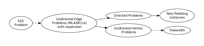
Figure 1: Overview of Reductions. Dashed arrows indicate that the reduction is obtained by the identity mapping, whereas solid arrows indicate a nontrivial transformation from one problem to the other.

Figure 1 gives a high-level overview of these reductions.

4 Hardness For Layout Problems

In this section, we show that all of the layout problems defined in Section 2.1 are SSE-hard to approximate within any constant factor. This also shows that pathwidth and the one-shot pebbling problems are hard to approximate within any constant.

4.1 Hardness for MCLA and MLA

In this section, we recall the proof of [RST10] for MLA, and observe that it applies for MCLA as well. For an undirected graph $G$, let us write $\operatorname{\sf{MCLA}}(G)$ (resp., $\operatorname{\sf{MLA}}(G)$) for the MCLA value (resp., MLA value) of $G$, i.e.,

$$\operatorname{\sf{MLA}}(G) =\operatorname{\sf{Layout}}(G;E,\Sigma)=\min_{\pi}\sum_{i\in[n]}|E_{i}(\pi)|$$

$$\operatorname{\sf{MCLA}}(G) =\operatorname{\sf{Layout}}(G;E,\max)=\min_{\pi}\max_{i\in[n]}|E_{i}(\pi)|.$$

Theorem 4.1.

For every $\epsilon>0$, given a graph $G=(V,E)$, it is SSE-hard to distinguish between:

Yes

$\operatorname{\sf{MLA}}(G)\leq O(\epsilon\cdot|V|\cdot|E|)$ and $\operatorname{\sf{MCLA}}(G)\leq O(\epsilon|E|)$

No

For every $S\subseteq V$ with $|V|/10\leq|S|\leq 9|V|/10$, it holds that $|E(S,V\setminus S)|\geq\Omega(\sqrt{\epsilon}|E|)$. In particular, $\operatorname{\sf{MLA}}(G)\geq\Omega(\sqrt{\epsilon}\cdot|V|\cdot|E|)$ and $\operatorname{\sf{MCLA}}(G)\geq\Omega(\sqrt{\epsilon}|E|)$.

Proof.

We use the instances for Conjecture 2.19 with $q=1/\epsilon$. Let $G=(V,E)$ be an instance for Conjecture 2.19.

In the Yes case, we have disjoint sets $S_{1},\ldots,S_{q}$ and for each set $S_{j}$, $|S_{j}|=n/q=\epsilon n$, $\Phi_{G}(S_{j})\leq 2\epsilon$. We give an ordering $\pi$ of the vertices such that $\max_{i\in[n]}|E_{i}(\pi)|\leq 3\epsilon|E|$ as follows. Order the vertices as $S_{1},\ldots,S_{q}$ (with the order within each $S_{j}$ chosen arbitrary) and let this order be $\pi$. For any $i\in[n]$, we show that $|E_{i}(\pi)|\leq 3\epsilon|E|$. Suppose $\pi^{-1}(i)$ is a vertex in $S_{j}$. Each edge in $E_{i}(\pi)$ either has both end-points inside $S_{j}$, or its end-points in two different $S_{k}$’s. The total number of edges inside $S_{j}$ is at most $\epsilon dn/2=\epsilon|E|$. Moreover, by Remark 2.20, the total number of edges with end-points in two different $S_{k}$’s is at most $2\epsilon|E|$. Therefore, $\operatorname{\sf{MCLA}}(G)\leq\max_{i}|E_{i}(\pi)|\leq 3\epsilon|E_{i}(\pi)|$. The $\operatorname{\sf{MLA}}$ value can be bounded similarly.

The property of the No instance is the same as in Conjecture 2.19 (via Remark 2.21), and the implications for the $\operatorname{\sf{MLA}}$ and $\operatorname{\sf{MCLA}}$ values are immediate. ∎

4.2 Reduction To Directed Graphs

Given an undirected graph $G=(V,E)$, we construct a directed graph $D=(V^{\prime},E^{\prime})$ as follows. In order to distinguish the elements of $V$ and $E$ from the elements of $V^{\prime}$ and $E^{\prime}$, we refer to elements of $V$ as vertices, elements of $E$ as edges, elements of $V^{\prime}$ as nodes, and elements of $E^{\prime}$ as arcs.

There is a node in $D$ for each vertex and for each edge of $G$, i.e., $V^{\prime}=V\cup E$. The graph $D$ is bipartite with bipartition $V,E$, and there is an arc in $D$ from $e\in E$ to $v\in V$ if $e$ is incident upon $v$. Formally,

$$V^{\prime} = V\cup E$$

$$E^{\prime} = \{(e,v)\,|\,e\in E,v\in V,v\in e\}.$$

See also Figure 2.

Figure 2: The reduction from $G$ to $D$.

The remainder of this section is devoted to analyzing the reduction. First, it is easy to give an upper bound on the four $\operatorname{\sf{Layout}}$ values of $D$ in terms of the $\operatorname{\sf{MLA}}$ and $\operatorname{\sf{MCLA}}$ values of $G$.

Lemma 4.2.

The DAG $D$ constructed from $G$ as above satisfies the following:

$$\operatorname{\sf{Layout}}(D;E,\Sigma) \leq\left(\operatorname{\sf{MLA}}(G)+O(|E|)\right)\cdot(d+1)$$

$$\operatorname{\sf{Layout}}(D;E,\max) \leq\operatorname{\sf{MCLA}}(G)+d.$$

Note that, for the purposes of applying this to the graphs of Theorem 4.1 the error term of $|E|$ (resp. $d$) is insignifcant compared to the $\operatorname{\sf{MLA}}$ (resp. $\operatorname{\sf{MCLA}}$) value of $G$.

Proof.

Consider an ordering $\pi$ of $V$. For a set of vertices $S$ of $V$, let $u_{\pi}(S)\in S$ denote the vertex of $S$ that comes first in the ordering $\pi$.

We extend $\pi$ to an ordering $\pi^{\prime}$ of $V^{\prime}$ by inserting each edge $e=(u,v)$ immediately before the vertex $u_{\pi}(e)$. It is easy to see that for each node $z\in V^{\prime}\cup E^{\prime}$,

$$|E_{z}(\pi^{\prime})| \leq|E_{u_{\pi}(z)}(\pi)|+d$$

This immediately implies

$$\operatorname{\sf{Layout}}(D;E,\max)\leq\max_{z\in V^{\prime}}|E_{z}(\pi^{\prime})|\leq\max_{u\in V}|E_{u}(\pi)|+d,$$

Setting $\pi$ to be an optimal MCLA ordering of $G$, we obtain the second claim of the Lemma. Similarly, using that $|u^{-1}(v)|\leq d+1$ for every $v\in V$, we get

$$\operatorname{\sf{Layout}}(D;E,\Sigma)\leq\sum_{z\in V^{\prime}}|E_{z}(\pi^{\prime})|\leq(d+1)\sum_{u\in V}|E_{u}(\pi)|+d|V^{\prime}|,$$

Setting $\pi$ to be an optimal MLA ordering of $G$ and using $|V^{\prime}|=O(|E|)$, we obtain the first claim of the Lemma. ∎

Next we use the strong soundness property of Theorem 4.1 to argue about the soundness of $D$.

Lemma 4.3.

Suppose $G$ has the property that for every $|V|/10\leq|S|\leq 9|V|/10$ we have $|E(S,V\setminus S)|\geq\Omega(\sqrt{\epsilon}|E|)$. Then,

$$\operatorname{\sf{Layout}}(D;V,\Sigma) \geq\Omega(\sqrt{\epsilon}|E|^{2})$$

$$\operatorname{\sf{Layout}}(D;V,\max) \geq\Omega(\sqrt{\epsilon}|E|)$$

Proof.

Let $\pi^{\prime}$ be any ordering of $V^{\prime}$. Using the expansion property of Theorem 4.1, we’ll show that this ordering must have high cost. For a point $i\in[N]$, let $S_{i}$ be the set of vertices of $V$ that appear after $i$ in $\pi^{\prime}$.

The bound on $\operatorname{\sf{Layout}}(D;V,\max)$ is immediate: consider a point $i\in[N]$ such that $|S_{i}|=|V|/2$. By the expansion property $|E(S_{i},V\setminus S_{i})|\geq\Omega(\sqrt{\epsilon}|E|)$, and since each such edge $e$ has one of its endpoints before point $i$, the node $e$ itself must appear before point $i$ and thus $|V_{i}(\pi^{\prime})|\geq|E(S_{i},V\setminus S_{i})|\geq\Omega(\sqrt{\epsilon}|E|)$.

Let us then turn to $\operatorname{\sf{Layout}}(D;V,\Sigma)$. Write $c_{i}$ for the fraction of edges $e$ that appear before (or at) point $i$ in $\pi^{\prime}$. We shall show that whenever $1/5\leq c_{i}\leq 4/5$, we have $|V_{i}(\pi^{\prime})|\geq\Omega(\sqrt{\epsilon}|E|)$, giving a total of $\operatorname{\sf{Layout}}(D;V,\Sigma)\geq\Omega(\sqrt{\epsilon}|E|^{2})$.

By a simple counting argument, we have

$$d|S_{i}|\geq 2(1-c_{i})|E|,$$

implying $|S_{i}|\geq(1-c_{i})|V|$ which for $c_{i}\leq 4/5$ is at least a $1/5$ fraction of vertices. If in addition $|S_{i}|\leq 9|V|/10$, the argument above gives $|V_{i}(\pi^{\prime})|\geq\Omega(\sqrt{\epsilon}|E|)$. The remaining case is that $|S_{i}|\geq 9|V|/10$. But then $S_{i}$ is incident upon at least a $9/10$ fraction of edges. This implies that the number of edges incident upon $S_{i}$, appearing before $i$ in $\pi^{\prime}$, are at least $|E|(c_{i}-1/10)$ which for $c_{i}\geq 1/5$ is $\Omega(\sqrt{\epsilon}|E|)$. ∎

Combining Lemma 4.2 and Lemma 4.3, with Theorem 4.1, and using the fact that edge costs are always larger than the corresponding vertex costs, we immediately obtain the following theorem.

Theorem 4.4.

Given a DAG $D$, $\operatorname{\sf{Layout}}(D;E,\max)$, $\operatorname{\sf{Layout}}(D;E,\Sigma)$, $\operatorname{\sf{Layout}}(D;V,\max)$, and $\operatorname{\sf{Layout}}(D;V,\Sigma)$ are all SSE-hard to approximate within any constant factor, even in DAG’s with maximum path length $1$ (i.e., every vertex is a source or a sink).

Remark 4.5.

In fact we see that, as in Theorem 4.1, the four hardness results applies to the same instance, so that it is SSE-hard to distinguish all of the four $\operatorname{\sf{Layout}}$ values being high from all of them being low.

As the one-shot black pebbling problem is precisely $\operatorname{\sf{Layout}}(D;V,\max)$, we obtain hardness for one-shot black pebbling as an immediate corollary. However, the instances are not single-sink DAGs with maximum indegree $2$, as promised in Theorem 1.2. In Section 6 we show how to transform the instances further to obtain such DAGs.

4.3 Undirected Vertex Problems

The reduction for undirected vertex problems is very similar to the reduction for directed problems given in the previous section. As before, we introduce nodes for every edge of $G$. As in the directed case, we are interested in orderings where an edge appears before its two endpoints, but we cannot use direction to force this anymore. Instead, we ensure that orderings that are not like this incur a high cost by replicating each node corresponding to a vertex of $G$ many times.

Given an undirected graph $G=(V,E)$, we construct a new graph $G^{\prime}=(V^{\prime},E^{\prime})$ as follows.

There are $r$ nodes in $G^{\prime}$ for each vertex and one node for each edge of $G$, i.e., $V^{\prime}=V\times[r]\cup E$. For a vertex $u\in V$ we write $u^{1},\ldots,u^{r}$ to denote the $r$ copies of $u$ and refer to each such set of $r$ nodes as a vertex group. The graph $G^{\prime}$ is bipartite with bipartition $V\times[r],E$, and there is an edge in $G^{\prime}$ between $e\in E$ and $v^{i}\in V\times[r]$ if $e$ is incident upon $v$. Formally,

$$V^{\prime} = \{v^{i}\,|\,v\in V,i\in[r]\}$$

$$E^{\prime} = \{(e,v^{i})\,|\,e\in E,v\in V,v\in e,i\in[r]\}.$$

See also Figure 3.

Figure 3: The reduction from $G$ to $G^{\prime}$, illustrated for $r=3$.

Lemma 4.6.

The graph $G^{\prime}$ constructed from $G$ as above satisfies the following:

$$\operatorname{\sf{Layout}}(G^{\prime};V,\Sigma) \leq(d+r)\operatorname{\sf{MLA}}(G)$$

$$\operatorname{\sf{Layout}}(G^{\prime};V,\max) \leq\operatorname{\sf{MCLA}}(G).$$

Proof.

We proceed as in the proof of Lemma 4.2. An ordering $\pi$ of $V$ naturally induces an ordering $\pi^{\prime}$ of $V^{\prime}$: put all $r$ copies of $u\in V$ consecutively, with vertices of $V$ appearing in the same order as in $\pi$, and insert each edge $e\in E$ immediately before its first vertex. Again, for an edge $e\in E$, let $u_{\pi}(z)$ denote the endpoint of $e$ that appears first in $\pi$. Similarly, for a copy $v^{i}\in V^{\prime}$ of $v\in V$, let $u_{\pi}(v^{i})=v$. It is easy to see that the constructed ordering $\pi^{\prime}$ satisfies

$$|V_{z}(\pi^{\prime})| \leq|E_{u_{\pi}(z)}(\pi)|$$

for every $z\in V^{\prime}$. This immediately implies

$$\operatorname{\sf{Layout}}(G^{\prime};V,\max)\leq\max_{z\in V^{\prime}}|V_{z}(\pi^{\prime})|\leq\max_{u\in V}|E_{u}(\pi)|,$$

Similarly, we get

$$\operatorname{\sf{Layout}}(G^{\prime};V,\Sigma)\leq\sum_{z\in V^{\prime}}|V_{z}(\pi^{\prime})|\leq(d+r)\sum_{u\in V}|E_{u}(\pi)|.$$

∎

Lemma 4.7.

Suppose $G$ has the property that for every $|V|/10\leq|S|\leq 9|V|/10$ we have $|E(S,V\setminus S)|\geq\Omega(\sqrt{\epsilon}|E|)$. Then, if $r\geq|V|\cdot|E|$, we have

$$\operatorname{\sf{Layout}}(G^{\prime};V,\Sigma) \geq\Omega(\sqrt{\epsilon}\cdot r\cdot|V|\cdot|E|)$$

$$\operatorname{\sf{Layout}}(G^{\prime};V,\max) \geq\Omega(\sqrt{\epsilon}|E|)$$

Proof.

Let $\pi^{\prime}$ be an ordering of $V^{\prime}$. First we have the following simple claim, establishing that for good orderings, most vertices appear after their edges.

Claim 4.8.

Suppose that for some vertex $u\in V$, at least $r/2$ of the copies of $u$ in $G^{\prime}$ appear before some edge $e=(u,v)\in E$ adjacent upon $u$. Then

$$\max_{i\in[N]}|V_{i}(\pi^{\prime})| \geq r/4\gg\Omega(\sqrt{\epsilon}\cdot|E|)$$

$$\sum_{i\in[N]}|V_{i}(\pi^{\prime})| \geq(r/4)^{2}\gg\Omega(\sqrt{\epsilon}\cdot r\cdot|V|\cdot|E|).$$

Proof.

Let $I_{1}$ be the first half of the positions where copies of $u$ appear before $e$, and $I_{2}$ the second half. Thus, $|I_{1}|,|I_{2}|\geq r/4$. Then each element of $I_{1}$ contributes to $V_{i}(\pi^{\prime})$ for each $i\in I_{2}$, giving the claimed bounds. ∎

Thus we may without loss of generality assume that for each vertex $u$ of $V$, at least $r/2$ of its $r$ copies in $G^{\prime}$ appear after all edges adjacent upon $u$. From now on, let us discard all the $\leq r/2$ “bad” copies of each vertex of $V$ that appear before some of its edges. This only decreases the cost of $\pi^{\prime}$, and there are still $\geq r|V|/2$ vertex nodes left.

Let $i_{1}$ be the (first) point of $\pi^{\prime}$ such that $r|V|/10$ vertex nodes are to the left of $i_{1}$, and $i_{2}$ the (last) point of $\pi^{\prime}$ such that $r|V|/10$ vertex nodes are to the right of $i_{2}$.

Claim 4.9.

For any point $i$ between $i_{1}$ and $i_{2}$, we have $|V_{i}(\pi^{\prime})|\geq\Omega(\sqrt{\epsilon}|E|)$.

Proof.

Let $S\subseteq V$ (resp. $T\subseteq V$) be the set of vertices $u$ such that some copy of $u$ appears before $i$ (resp. after $i$). We then have $|S|,|T|\geq\frac{r|V|/10}{r/2}\geq|V|/5$, and $S\cup T=V$. Thus we can partition $V$ into $S^{\prime}\subseteq S,T^{\prime}\subseteq T$ such that $|S^{\prime}|,|T^{\prime}|\leq 4|V|/5$. By the expansion property of $G$ we have $|E(S^{\prime},T^{\prime})|\geq\Omega(\sqrt{\epsilon}|E|)$. Further, we also have $|V_{i}(\pi^{\prime})|\geq|E(S^{\prime},T^{\prime})|$ as each $e\in E(S^{\prime},T^{\prime})$ must appear before $i$ in $\pi^{\prime}$ (because one of their endpoints is in $S$) but have an edge crossing $i$ (because the other of their endpoints is in $T$). ∎

From Claim 4.9, the proof of the lemma follows immediately. ∎

As in the previous section, we can now combine Lemma 4.6 and Lemma 4.7, with Theorem 4.1, to obtain:

Theorem 4.10.

Given a graph $G$, $\operatorname{\sf{Layout}}(G;V,\max)$, $\operatorname{\sf{Layout}}(G;V,\Sigma)$ are both SSE-hard to approximate within any constant factor, even in bipartite graphs.

As the pathwidth problem is precisely $\operatorname{\sf{Layout}}(G;V,\max)$, we obtain hardness for pathwidth as an immediate corollary. In the next section, we’ll show the stronger soundness required for Theorem 1.1.

5 Hardness For Treewidth

In this section we shall complete our proof of Theorem 1.1 by showing that the hard instances for pathwidth from Theorem 4.10 also have large treewidth.

Lemma 5.1.

Let $G=(V,E)$ be an undirected graph with the property that for every $|V|/10\leq|S|\leq 9|V|/10$ we have $|E(S,V\setminus S)|\geq\Omega(\sqrt{\epsilon}|E|)$, and let $G^{\prime}$ be the graph obtained by applying the reduction of Section 4.3 to $G$. Then, if $r\geq|V|\cdot|E|$, we have

$$\operatorname{\sf{tw}}(G^{\prime}) \geq\Omega(\sqrt{\epsilon}|E|)$$

To prove Lemma 5.1, we shall use the fact that the treewidth of a graph is closely related to an expansion-like property called the $1/2$-separator number, defined in [BGHK95].

Definition 5.2 (1/2-vertex separator, 1/2-separator number).

Let $G=(V,E)$ be an undirected graph. For $W\subseteq V$, a $1/2$-vertex separator of $W$ in $G$ is a set $S\subseteq V$ of vertices such that every connected component of the graph $G[V-S]$ contains at most $|W|/2$ vertices of $W$. Let $\psi_{G}(1/2,W)$ denote the minimum size of a 1/2-vertex separator of $W$ in $G$. We define the 1/2-separator number $K_{1/2}(G)$ to be

$$K_{1/2}(G)=\max_{W\subseteq V}\psi_{G}(1/2,W).$$

Lemma 5.3 ([BGHK95]).

For every graph $G=(V,E)$, it holds that $\operatorname{\sf{tw}}(G)\geq K_{1/2}(G)-1$.

Using this, it is now straightforward to prove the lower bound on the treewidth.

Proof of Lemma 5.1.

We’ll show that $\psi_{G^{\prime}}(1/2,V^{\prime})\geq\Omega(\sqrt{\epsilon}|E|)$ (i.e. we choose $W=V^{\prime}$). Suppose $C$ is an optimal $1/2$-vertex separator of $V^{\prime}$ and it separates $V^{\prime}\setminus C$ into $l$ sets $V_{1}^{\prime},\ldots,V_{l}^{\prime}$, each of size at most $|V^{\prime}|/2$. By merging different $V_{i}^{\prime}$ we may assume that we only have two sets $V_{1}^{\prime}$ and $V_{2}^{\prime}$, both of size at least $|V^{\prime}|/5$.

Now, similarly to the proof of Claim 4.9, let $S\subseteq V$ (resp. $T\subseteq V$) be the set of vertices $v$ such that some copy of $V$ appears in $V_{1}^{\prime}$ (resp. $V_{2}^{\prime}$). As $|V_{1}^{\prime}|,|V_{2}^{\prime}|\geq r|V|/5$, this implies that both $|S|,|T|$ are at least $|V|/5$, and furthermore $S\cup T=V$ (since otherwise all $r$ copies of some vertex are in $C$, implying $|C|\geq r\gg\Omega(\sqrt{\epsilon}|E|)$). We can thus choose a balanced partition $S^{\prime},T^{\prime}$ such that $S^{\prime}\subseteq S$, $T^{\prime}\subseteq T$, and we have $|E(S^{\prime},T^{\prime})|\geq\Omega(\sqrt{\epsilon}|E|)$. But every edge $e=(u,v)$ such that $u\in S^{\prime}$ and $v\in T^{\prime}$ must belong to $C$, since it is connected (in $G^{\prime}$) to every copy of $u$ and $v$. ∎

6 Nicer Pebbling Instances

In this section we show how to transform our hard instances for one-shot black pebbling so as to have in-degree bounded by $2$ and single sinks.

We begin with the in-degree.

Lemma 6.1.

Given a DAG $D=(V,E)$ we can in polynomial time construct a DAG $D^{\prime}=(V^{\prime},E^{\prime})$ such that every node of $D^{\prime}$ has in-degree at most $2$ and

$${\sf BP}^{1{\sf s}}(D)\leq{\sf BP}^{1{\sf s}}(D^{\prime})\leq{\sf BP}^{1{\sf s}}(D)+d,$$

where $d$ is the maximum in-degree of $D$.

As the proof of this lemma is somewhat lengthy, we defer it until later in this section and first describe how to obtain a DAG with a single sink.

Lemma 6.2.

Given a DAG $D=(V,E)$ we can in polynomial time construct a DAG $D^{\prime}=(V^{\prime},E^{\prime})$ such that $D^{\prime}$ has a single sink and

$${\sf BP}^{1{\sf s}}(D)\leq{\sf BP}^{1{\sf s}}(D^{\prime})\leq{\sf BP}^{1{\sf s}}(D)+s+1,$$

where $s$ is the number of sinks in $D$. Furthermore, if $D$ has maximum in-degree $2$ then so does $D^{\prime}$.

Proof.

Construct $D^{\prime}$ by adding a binary tree with $s$ leaves to $D$, and identifying the leaves of the tree with the sinks of $D$. The properties of $D^{\prime}$ are easily verified. Since $D^{\prime}$ is a super-DAG of $D$, its pebbling cost must be at least ${\sf BP}^{1{\sf s}}(D)$. Conversely, a valid pebbling of $D^{\prime}$ can be obtained by using a one-shot pebbling of $D$ but without removing pebbles from the sinks, and then pebbling the tree. ∎

Given Lemmas 6.1 and 6.2 we can derive Theorem 1.2. The point is that for the graphs produced in Theorem 4.4, the maximum indegree $d$ equals the degree of the original SSE instance, and the number of sinks $s$ equals the number of vertices of the original pebbling instance. On the other hand, the one-shot black pebbling cost (i.e., the $\operatorname{\sf{Layout}}(D;V,\max)$ value) is of order $\epsilon|E|$ which is much larger than $d$ and $s$, so the additive losses of Lemmas 6.1 and 6.2 are insignificant. We omit the details.

6.1 Lemma 6.1

In this section we prove Lemma 6.1. First, recall the definition of a pyramid graph.

Figure 4: Pyramid of size $4$

Definition 6.3.

A pyramid graph of size $d$ is a layered graph of indegree two, with $d$ layers, labelled $0,1,\ldots,d-1$. Layer zero (the input layer) consists of $d$ vertices, and layer $i$ contains $d-i$ vertices. See Figure 4.

Figure 5: Reduction to DAGs of indegree $2$

The reduction of Lemma 6.1 to produce DAGs of indegree $2$ is as follows. Construct $D^{\prime}$ by replacing each vertex $u$ by a pyramid $P_{u}$ of size $d(u)$ (here, $d(u)$ denotes the indegree of $u$), where the $d(u)$ vertices at layer $0$ of $P_{u}$ are identified with the predecessors of $u$, and $u$ is identified with the vertex at layer $d(u)-1$ of $P_{u}$. See Figure 5.

To prove the lemma we need to show that $D^{\prime}$ constructed this way satisfies

$${\sf BP}^{1{\sf s}}(D)\leq{\sf BP}^{1{\sf s}}(D^{\prime})\leq{\sf BP}^{1{\sf s}}(D^{\prime})+d,$$

where $d$ is the maximum indegree of any vertex $u$ of $D$.

In what follows whenever we say “pebbling strategy” of $D$ or $D^{\prime}$ we always refer to a one-shot black pebbling strategy of $D$ or $D^{\prime}$.

The upper bound on ${\sf BP}^{1{\sf s}}(D^{\prime})$ is trivial: if $S$ is a valid pebbling strategy for $D$, then clearly we can create a corresponding pebbling strategy for $D^{\prime}$ by pebbling through the pyramid whenever $D$ pebbles the sink of the pyramid. This takes at most $d$ additional pebbles.

In the other direction, we want to show that a pebbling strategy for $D^{\prime}$ can be converted into a pebbling strategy for $D$. We will first show that $D^{\prime}$ can be assumed to be in a particular normal form, and then using this normal form, we will show how to simulate the pebbling.

Definition 6.4.

Let $S^{\prime}$ be a pebbling strategy of $D^{\prime}$. That is, $S^{\prime}$ is a sequence of configurations, where each configuration is a set of black pebble placements, and such that the sequence of configurations follows by the black pebbling rules. We say that configuration $c\in S^{\prime}$ is saturated with respect to a pyramid $P_{u}$ if $c$ is the first time in $S^{\prime}$ that there is a black pebble path cutting the sink of $P_{u}$ from all of the sources of $P_{u}$. (The cut does not include any sources or the sink of $P_{u}$.) Note that this cut has size $d-1$.

Claim 6.5.

Let $S^{\prime}$ be a pebbling strategy for $D^{\prime}$. We can assume without loss of generality that $D^{\prime}$ has the following normal form. For each configuration $c^{\prime}\in S^{\prime}$, if $c^{\prime}$ is saturated with respect to pyramid $P_{u}$, then the subsequent moves of $S^{\prime}$ pebble the sink of $P_{u}$ (in the obvious way), removing all other black pebbles on the internal nodes of $P_{u}$.

Proof Sketch.

At a saturated configuration $c^{\prime}$, there must be $d-1$ pebbles on internal nodes of $P_{u}$. If we subsequently pebble the sink of $p$, we will never use more than $d-1$ pebbles on internal nodes of $p$, and all other pebbles on the graph stay as they were. Thus the normal form does not use more pebbles than the original strategy. Furthermore, since the internal nodes of a pyramid are only used to pebble the sink of this pyramid, we have not lost anything by pebbling through to the sink and removing the other internal black pebbles. ∎

From now on we will assume that the pebbling $S^{\prime}$ of $D^{\prime}$ has the above normal form. That is, if a configuration is saturated (with respect to a pyramid $P_{u}$), the next thing that happens in $S^{\prime}$ is to pebble the sink of $P_{u}$. (After pebbling the sink, we will have not touched whatever pebbles were on the source nodes of $P_{u}$, and we will have a pebble on the sink node of $P_{u}$, and no other internal pebbles on $P_{u}$.)

Our strategy for constructing a pebbling, $S$, of $D$, given a normal form pebbling, $S^{\prime}$ of $D^{\prime}$ is as follows. For each node $v$ of $D$, pebble $v$ whenever it is first pebbled in $S^{\prime}$, and remove the pebble from $v$ as soon as all successors of $v$ (in the original graph $D$) are pebbled. We want to argue that this pebbling strategy of $D$ is not greater than that of $D^{\prime}$. To see this, we will use the following Lemma.

Lemma 6.6.

In any frugal read-once black strategy of a size $d$ pyramid, the number of pebbles on the pyramid at any point in time, up until all sources are pebbled for the first time, must be equal to the number of sources in that pyramid that have been pebbled so far.

Assuming the above Lemma it is clear that if $S^{\prime}$ is a normal form pebbling of $D^{\prime}$, then for any pyramid $p$ in $D^{\prime}$, and any configuration $c^{\prime}$, if there are $k$ pebbles on $P_{u}$ at $c^{\prime}$, then in the corresponding configuration $c$ of $D$, there are at most $k$ pebbles on source nodes of $P_{u}$. To see this, first notice that by the above Lemma, anytime a pyramid is being pebbled in $D^{\prime}$ up until the time when all source nodes of the pyramid are pebbled for the first time, the number of pebbles on the pyramid will be at least as large as the number of source nodes in $D$ that contain pebbles. Then by the normal form property of $D^{\prime}$, as soon as all source nodes of $D^{\prime}$ are pebbled for the first time, the strategy pebbles the sink of $D^{\prime}$, and thus again the number of corresponding pebbles on $D$ is never greater than the number of pebbles on $D^{\prime}$.

Proof of Lemma 6.6.

Let $P$ be a size $d$ pyramid graph, and let $S$ a one-shot black pebbling of $P$. Let $c$ be a configuration occuring in $S$ such that the set of source nodes that have been pebbled up to $c$ are the source nodes of $P^{\prime}$, where $P^{\prime}$ is a size $d^{\prime}$ sub-pyramid of $P$. We want to argue that $c$ must contain at least $d^{\prime}$ pebbles. Assume without loss of generality that $P^{\prime}$ is the leftmost sub-pyramid of $P$, of size $d^{\prime}<d$. Label the outer rightmost vertices of $P^{\prime}$ by $v_{d-1},...,v_{0}$, where $v_{d-1}$ is the sink vertex of $P^{\prime}$, and for all $i<d-1$, $v_{i}$ is the rightmost vertex in $P^{\prime}$ at level $i$. Corresponding to each named vertex $v_{i}$ is a diagonal set of vertices, $diag(v_{i})$, beginning at $v_{i}$ and travelling southwest to a source vertex of $P^{\prime}$. Note that the sets $diag(v_{i})$ are pairwise disjoint. We will argue that for each $i$, $0\leq i\leq d-1$, at least one vertex from $diag(v_{i})$ must appear in $c$. To see this, first notice that for each $v_{i}$, there is a vertex $v_{i}^{\prime}$ that is an immediate successor of $v_{i}$ and that lies outside of $P^{\prime}$. This vertex $v_{i}^{\prime}$ must be pebbled at some time after configuration $c$, since it has a predecessor that has not yet been pebbled. But in order to pebble $v_{i}^{\prime}$ in the future, there must be a black pebble on some vertex in $diag(v_{i})$ in $c$. Thus, we have shown that if $c$ is any configuration in $S$ such that $d^{\prime}<d$ source vertices are pebbled thus far, then there must be $d^{\prime}$ vertices pebbled in $c$. ∎

7 Conclusion and Open Problems

We proved SSE-hardness of approximation for a variety of graph problems. Most importantly we obtained the first inapproximability result for the treewidth problem.

Some remarks are in order. The status of the SSE conjecture is, at this point in time, very uncertain, and our results should therefore not be taken as absolute evidence that there is no polynomial time approximation for (e.g.) treewidth. However, at the very least, our results do give an indication of the difficulty involved in obtaining such an algorithm for treewidth, and builds a connection between these two important problems. We also find it remarkable how simple our reductions and proofs are. We leave the choice of whether to view this as a healthy sign of strength of the SSE Conjecture, or whether to view it as an indication that the conjecture is too strong, to the reader.

There are many important open questions and natural avenues for further work, including:

1. It seems plausible that these results can be extended to a wider range of graph layout problems. For instance, our two choices of aggregators $\max$ and $\Sigma$ can be viewed as taking $\ell_{\infty}$ and $\ell_{1}$ norms, and it seems likely that the results would apply for any $\ell_{p}$ norm (though we are not aware of any previous literature studying such variants).

2. It would be nice to obtain hardness of approximation result for our problems based on a weaker hardness assumption such as UGC. It is conjectured in [RST10] that the SSE conjecture is equivalent to UGC. Alternatively, it would be nice to show that hardness of some of our problems imply hardness for the SSE Problem.

3. For pebbling, it would be very interesting to obtain results for the unrestricted pebbling problems (for which finding the exact pebbling cost is even PSPACE-hard). As far as we are aware, nothing is known for these problems, not even, say, whether one can obtain a non-trivial approximation in NP. As mentioned in the introduction, we are currently working on extending our one-shot pebbling results to bounded time pebblings. We have some preliminary progress there and are hopeful that we can relax the pebbling results to a much larger class of pebblings.

References

- [ABS10] Sanjeev Arora, Boaz Barak, and David Steurer. ”subexponential algorithms for unique games and related problems”. In FOCS, pages 563–572, 2010.
- [ACMM05] Amit Agarwal, Moses Charikar, Konstantin Makarychev, and Yury Makarychev. approximation algorithms for min UnCut, min 2CNF deletion, and directed cut problems. In Proceedings of the thirty-seventh annual ACM symposium on Theory of computing, STOC ’05, pages 573–581, New York, NY, USA, 2005. ACM.
- [ACP87] Stefan Arnborg, Derek G. Corneil, and Andrzej Proskurowski. Complexity of finding embeddings in a k-tree. SIAM J. Algebraic Discrete Methods, 8:277–284, April 1987.
- [AMS07] Christoph Ambuhl, Monaldo Mastrolilli, and Ola Svensson. Inapproximability Results for Sparsest Cut, Optimal Linear Arrangement, and Precedence Constrained Scheduling. In Proceedings of the 48th Annual IEEE Symposium on Foundations of Computer Science, pages 329–337, Washington, DC, USA, 2007. IEEE Computer Society.
- [ARV09] Sanjeev Arora, Satish Rao, and Umesh Vazirani. Expander flows, geometric embeddings and graph partitioning. J. ACM, 56:5:1–5:37, April 2009.
- [BGHK95] H. L. Bodlaender, J. R. Gilbert, H. Hafsteinsson, and T. Kloks. Approximating treewidth, pathwidth, frontsize, and shortest elimination tree. Journal of Algorithms, 18(2):238–255, 1995.
- [Bod96] Hans L. Bodlaender. A Linear-Time Algorithm for Finding Tree-Decompositions of Small Treewidth. SIAM J. Comput., 25(6):1305–1317, 1996.
- [Bod05] Hans L. Bodlaender. Discovering treewidth. In SOFSEM, pages 1–16, 2005.
- [Bod07] Hans Bodlaender. Treewidth: Structure and algorithms. In Giuseppe Prencipe and Shmuel Zaks, editors, Structural Information and Communication Complexity, volume 4474 of Lecture Notes in Computer Science, pages 11–25. Springer Berlin / Heidelberg, 2007. 10.1007/978-3-540-72951-8_3.
- [BRS11] Boaz Barak, Prasad Raghavendra, and David Steurer. ”rounding semidefinite programming hierarchies via global correlation”. ECCC Report TR11-065, 2011.
- [BT03] Vincent Bouchitté and Ioan Todinca. Approximating the treewidth of at-free graphs. Discrete Applied Mathematics, 131(1):11–37, 2003.
- [CHKR10] Moses Charikar, Mohammad Hajiaghayi, Howard Karloff, and Satish Rao. spreading metrics for vertex ordering problems. Algorithmica, 56:577–604, 2010.
- [Cou90] Bruno Courcelle. Graph Rewriting: An Algebraic and Logic Approach. In Handbook of Theoretical Computer Science, Volume B: Formal Models and Sematics (B), pages 193–242. 1990.
- [DFU11] Chandan K. Dubey, Uriel Feige, and Walter Unger. Hardness results for approximating the bandwidth. J. Comput. Syst. Sci., 77(1):62–90, 2011.
- [FHL05] Uriel Feige, MohammadTaghi Hajiaghayi, and James R. Lee. Improved approximation algorithms for minimum-weight vertex separators. In Proceedings of the thirty-seventh annual ACM symposium on Theory of computing, STOC ’05, pages 563–572, New York, NY, USA, 2005. ACM.
- [GS11] Venkatesan Guruswami and Ali Kemal Sinop. ”lasserre hierarchy, higher eigenvalues, and approximation schemes for quadratic integer programming with psd objectives”, 2011.
- [Kho02] Subhash Khot. On the power of unique 2-prover 1-round games. In Proceedings of the thiry-fourth annual ACM symposium on Theory of computing, STOC ’02, pages 767–775, New York, NY, USA, 2002. ACM.
- [Kin92] Nancy G. Kinnersley. The vertex separation number of a graph equals its path-width. Information Processing Letters, 42(6):345–350, 1992.
- [KP86] Lefteris M. Kirousis and Christos H. Papadimitriou. Searching and pebbling. Theor. Comput. Sci., 47:205–218, November 1986.
- [Len81] Thomas Lengauer. Black-white pebbles and graph separation. Acta Informatica, 16:465–475, 1981. 10.1007/BF00264496.
- [LR99] Tom Leighton and Satish Rao. Multicommodity max-flow min-cut theorems and their use in designing approximation algorithms. J. ACM, 46:787–832, November 1999.
- [LT82] Thomas Lengauer and Robert E. Tarjan. Asymptotically tight bounds on time-space trade-offs in a pebble game. J. ACM, 29:1087–1130, October 1982.
- [Nor10] Jakob Nordström. New wine into old wineskins: A survey of some pebbling classics with supplemental results. Draft manuscript, November 2010.
- [RAK91] R. Ravi, Ajit Agrawal, and Philip Klein. Ordering problems approximated: single-processor scheduling and interval graph completion. In Javier Albert, Burkhard Monien, and Mario Artalejo, editors, Automata, Languages and Programming, volume 510 of Lecture Notes in Computer Science, pages 751–762. Springer Berlin / Heidelberg, 1991. 10.1007/3-540-54233-7180.
- [RR88] G. Ramalingam and C. Pandu Rangan. A unified approach to domination problems on interval graphs. Inf. Process. Lett., 27:271–274, April 1988.
- [RR98] Satish Rao and Andréa W. Richa. New approximation techniques for some ordering problems. In Proceedings of the ninth annual ACM-SIAM symposium on Discrete algorithms, SODA ’98, pages 211–218, Philadelphia, PA, USA, 1998. Society for Industrial and Applied Mathematics.
- [RS84] Neil Robertson and Paul D. Seymour. Graph minors. III. Planar tree-width. J. Comb. Theory, Ser. B, 36(1):49–64, 1984.
- [RS86] Neil Robertson and Paul D. Seymour. Graph minors. II. Algorithmic aspects of tree-width. Journal of Algorithms, 7(3):309–322, 1986.
- [RS10] Prasad Raghavendra and David Steurer. Graph expansion and the unique games conjecture. In Proceedings of the 42nd ACM symposium on Theory of computing, STOC ’10, pages 755–764, New York, NY, USA, 2010. ACM.
- [RST10] Prasad Raghavendra, David Steurer, and Madhur Tulsiani. Reductions Between Expansion Problems. ArXiv e-prints, November 2010.
- [Set73] Ravi Sethi. Complete register allocation problems. In Proceedings of the fifth annual ACM symposium on Theory of computing, STOC ’73, pages 182–195, New York, NY, USA, 1973. ACM.
- [ST94] Paul D. Seymour and Robin Thomas. Call routing and the ratcatcher. Combinatorica, 14(2):217–241, 1994.