IPMU-11-0110

Testing Little Higgs Mechanism at Future Colliders

Keisuke Harigaya(a), Shigeki Matsumoto(a),

Mihoko M. Nojiri(b,a) and Kohsaku Tobioka(a)

(a)IPMU, TODIAS, University of Tokyo, Kashiwa, 277-8583, Japan
(b)Theory Group, KEK, Tsukuba, 305-0801, Japan

1 Introduction

It is well known that the standard model (SM) has a serious problem called the little hierarchy problem [1], which is essentially from quadratically divergent corrections to the higgs mass term. The little higgs scenario [2] has been proposed to solve the problem. In the scenario, the higgs boson is regarded as a pseudo Nambu-Goldstone boson associated with a spontaneous breaking of a global symmetry at the energy scale of 𝒪(10)𝒪10{\cal O}(10) TeV. Explicit breaking terms of the symmetry are also specially arranged to cancel the quadratically divergent corrections at one-loop level. The mechanism of this cancellation is sometimes called the little higgs mechanism, which is commonly equipped in all models of the little higgs scenario.

The little higgs mechanism predicts the existence of new particles at the scale of 𝒪(1)𝒪1{\cal O}(1) TeV, which are called little higgs partners. The mechanism also predicts some relations between coupling constants of SM interactions and those of the new particles. Among the partners, the top partner is the most important one, because it is responsible for the cancelation of the largest quadratically divergent correction to the higgs mass term. The top partner has a color charge and could be produced in near future [3] at the large hadron collider (LHC) [4]. The discovery of the top partner, however, does not mean the confirmation of the little higgs scenario, because new particles which are similar to the top partner are also predicted in various new physics extensions of the SM[5]. In order to test the little higgs scenario, we have to verify the relation between interactions predicted by the little higgs mechanism.

This verification requires us to measure the Yukawa coupling of the top partner. Future linear colliders such as the international linear collider (ILC) [6] and the compact linear collider (CLIC) [7] give a good opportunity for coupling measurements [8]. Following four processes are considered in this article; higgs associated productions (e+eTT¯hsuperscript𝑒superscript𝑒𝑇¯𝑇e^{+}e^{-}\to T\bar{T}h, tT¯h+Tt¯h𝑡¯𝑇𝑇¯𝑡t\bar{T}h+T\bar{t}h) and threshold productions (e+eTT¯superscript𝑒superscript𝑒𝑇¯𝑇e^{+}e^{-}\to T\bar{T}, Tt¯+tT¯𝑇¯𝑡𝑡¯𝑇T\bar{t}+t\bar{T}), where t𝑡t, T𝑇T, and hh are top quark, top partner, and higgs boson, respectively. We found that the coupling can be measured precisely using the associate production e+eTT¯hsuperscript𝑒superscript𝑒𝑇¯𝑇e^{+}e^{-}\to T\bar{T}h when the center of mass energy is large enough. The threshold production e+eTT¯superscript𝑒superscript𝑒𝑇¯𝑇e^{+}e^{-}\to T\bar{T} also allows us to measure it with the same precision. Interestingly, with smaller center of mass energy, it is even possible to measure the coupling using the threshold production e+et¯T+Tt¯superscript𝑒superscript𝑒¯𝑡𝑇𝑇¯𝑡e^{+}e^{-}\to\bar{t}T+T\bar{t}.

This article is organized as follows. In the next section, we introduce the effective lagrangian to describe the top sector of the little higgs scenario. The little higgs mechanism is quantitatively described using the lagrangian. In sections 3 and 4, higgs associated and threshold productions of the top partner are discussed with particularly focusing on how the cross sections of these processes are sensitive to the Yukawa coupling of the top partner. In section 5, we consider how accurately the Yukawa coupling can be measured using the processes discussed in previous sections, and discuss the capability of future linear colliders to test the little higgs mechanism. Section 6 is devoted to summary of our discussions.

2 Top sector of the little higgs scenario

The method using an effective lagrangian is adopted to investigate the top sector of the little higgs scenario. In the following, we introduce the lagrangian and discuss what kinds of interactions are predicted from it. We finally mention our strategy to test the little higgs mechanism at future linear colliders such as the ILC.

2.1 Effective lagrangian

In the little higgs scenario, the vector-like quark called the top partner is necessarily introduced, which is responsible for the cancellation of quadratically divergent corrections to higgs mass term from the top quark [2]. Interactions between higgs boson, top quark, and top partner are described by the effective lagrangian,111For simplicity, we have omitted to write gauge interactions of third generation quarks and top partners in the effective lagrangian. See appendix A for the derivation of the lagrangian and its correspondence to specific little higgs models.

effsubscripteff\displaystyle{\cal L}_{\rm eff} =\displaystyle= mUU¯LURy3Q¯3LHcu3RyUQ¯3LHcURsubscript𝑚𝑈subscript¯𝑈𝐿subscript𝑈𝑅subscript𝑦3subscript¯𝑄3𝐿superscript𝐻𝑐subscript𝑢3𝑅subscript𝑦𝑈subscript¯𝑄3𝐿superscript𝐻𝑐subscript𝑈𝑅\displaystyle-m_{U}\bar{U}_{L}U_{R}-y_{3}\bar{Q}_{3L}H^{c}u_{3R}-y_{U}\bar{Q}_{3L}H^{c}U_{R} (1)
(λ/mU)U¯Lu3R|H|2(λ/mU)U¯LUR|H|2+h.c.,formulae-sequence𝜆subscript𝑚𝑈subscript¯𝑈𝐿subscript𝑢3𝑅superscript𝐻2superscript𝜆subscript𝑚𝑈subscript¯𝑈𝐿subscript𝑈𝑅superscript𝐻2𝑐\displaystyle-(\lambda/m_{U})\bar{U}_{L}u_{3R}|H|^{2}-(\lambda^{\prime}/m_{U})\bar{U}_{L}U_{R}|H|^{2}+h.c.,

where Q3L=(u3L,b3L)Tsubscript𝑄3𝐿superscriptsubscript𝑢3𝐿subscript𝑏3𝐿𝑇Q_{3L}=(u_{3L},b_{3L})^{T} and u3Rsubscript𝑢3𝑅u_{3R} are third generation left- and right-handed quarks, while ULsubscript𝑈𝐿U_{L} and URsubscript𝑈𝑅U_{R} are left- and right-handed top partners. Higgs boson is denoted by Hcsuperscript𝐻𝑐H^{c}, where the superscript ’c𝑐c’ denotes charge conjugation. Quantum numbers of these fields are shown in Table 1. Here, we postulate that top partners couple only to third generation quarks to avoid flavor changing processes. Model parameters mUsubscript𝑚𝑈m_{U}, y3subscript𝑦3y_{3}, yUsubscript𝑦𝑈y_{U} and λ𝜆\lambda are taken to be real by appropriate redefinitions of the fields. On the other hand, the parameter λsuperscript𝜆\lambda^{\prime} can be complex in general. We take, however, this parameter to also be real because of the little higgs mechanism discussed below.

Q3Lsubscript𝑄3𝐿Q_{3L} u3Rsubscript𝑢3𝑅u_{3R} ULsubscript𝑈𝐿U_{L} URsubscript𝑈𝑅U_{R} H𝐻H
SU(3)c 3 3 3 3 1
SU(2)L 2 1 1 1 2
U(1)Y 1/6 2/3 2/3 2/3 1/2
Table 1: Quantum numbers of Q3Lsubscript𝑄3𝐿Q_{3L}, u3Rsubscript𝑢3𝑅u_{3R}, ULsubscript𝑈𝐿U_{L}, URsubscript𝑈𝑅U_{R} and H𝐻H.

The little higgs mechanism at the top sector can be quantitatively defended by using the effective lagrangian in eq.(1). Since quadratically divergent corrections to the higgs mass term should be cancelled with each other at 1-loop level, the following relation between the coupling constants (y3subscript𝑦3y_{3}, yUsubscript𝑦𝑈y_{U}, and λsuperscript𝜆\lambda^{\prime}) is required,

2λ=y32+yU2,2superscript𝜆superscriptsubscript𝑦32superscriptsubscript𝑦𝑈2\displaystyle-2\lambda^{\prime}=y_{3}^{2}+y_{U}^{2}, (2)

which is nothing but the little higgs mechanism at the top sector. It is thus very important to confirm the relation experimentally. The purpose of this article is to clarify what kind of observation is the most efficient for this confirmation.

Once H𝐻H acquires the vacuum expectation value Hc=(v/2,0)delimited-⟨⟩superscript𝐻𝑐𝑣20\langle H^{c}\rangle=(v/\sqrt{2},0) with being v246similar-to-or-equals𝑣246v\simeq 246 GeV, the electroweak symmetry (SU(2)L×U(1)YSUsubscript2𝐿Usubscript1𝑌{\rm SU}(2)_{L}\times{\rm U}(1)_{Y}) is broken, and third generation quarks are mixed with top partners. Mass matrix of these particles is

(u¯3LU¯L)(ABCD)(u3RUR)=(t¯LT¯L)(mt00mT)(tRTR),matrixsubscript¯𝑢3𝐿subscript¯𝑈𝐿matrix𝐴𝐵𝐶𝐷matrixsubscript𝑢3𝑅subscript𝑈𝑅matrixsubscript¯𝑡𝐿subscript¯𝑇𝐿matrixsubscript𝑚𝑡00subscript𝑚𝑇matrixsubscript𝑡𝑅subscript𝑇𝑅\displaystyle\begin{pmatrix}\bar{u}_{3L}&\bar{U}_{L}\\ \end{pmatrix}\begin{pmatrix}A&B\\ C&D\\ \end{pmatrix}\begin{pmatrix}u_{3R}\\ U_{R}\\ \end{pmatrix}=\begin{pmatrix}\bar{t}_{L}&\bar{T}_{L}\\ \end{pmatrix}\begin{pmatrix}m_{t}&0\\ 0&m_{T}\\ \end{pmatrix}\begin{pmatrix}t_{R}\\ T_{R}\\ \end{pmatrix}, (3)

where A𝐴A, B𝐵B, C𝐶C, and D𝐷D are defined by Ay3v/2𝐴subscript𝑦3𝑣2A\equiv y_{3}v/\sqrt{2}, ByUv/2𝐵subscript𝑦𝑈𝑣2B\equiv y_{U}v/\sqrt{2}, Cλv2/(2mU)𝐶𝜆superscript𝑣22subscript𝑚𝑈C\equiv\lambda v^{2}/(2m_{U}), and DmU+λv2/(2mU)𝐷subscript𝑚𝑈superscript𝜆superscript𝑣22subscript𝑚𝑈D\equiv m_{U}+\lambda^{\prime}v^{2}/(2m_{U}), respectively. We call a Dirac fermion t𝑡t composed of tLsubscript𝑡𝐿t_{L} and tRsubscript𝑡𝑅t_{R} the top quark in following discussions. We also call T𝑇T the top partner which is defined by TLsubscript𝑇𝐿T_{L} and TRsubscript𝑇𝑅T_{R} in the same manner as t𝑡t. Mixing angles for left- and right-handed quarks to diagonarize the mass matrix are then defined by

(tLTL)=(cosθLsinθLsinθLcosθL)(u3LUL),(tRTR)=(cosθRsinθRsinθRcosθR)(u3RUR).formulae-sequencematrixsubscript𝑡𝐿subscript𝑇𝐿matrixcossubscript𝜃𝐿sinsubscript𝜃𝐿sinsubscript𝜃𝐿cossubscript𝜃𝐿matrixsubscript𝑢3𝐿subscript𝑈𝐿matrixsubscript𝑡𝑅subscript𝑇𝑅matrixcossubscript𝜃𝑅sinsubscript𝜃𝑅sinsubscript𝜃𝑅cossubscript𝜃𝑅matrixsubscript𝑢3𝑅subscript𝑈𝑅\displaystyle\begin{pmatrix}t_{L}\\ T_{L}\\ \end{pmatrix}=\begin{pmatrix}{\rm cos}\theta_{L}&-{\rm sin}\theta_{L}\\ {\rm sin}\theta_{L}&{\rm cos}\theta_{L}\\ \end{pmatrix}\begin{pmatrix}u_{3L}\\ U_{L}\\ \end{pmatrix},\qquad\begin{pmatrix}t_{R}\\ T_{R}\\ \end{pmatrix}=\begin{pmatrix}{\rm cos}\theta_{R}&-{\rm sin}\theta_{R}\\ {\rm sin}\theta_{R}&{\rm cos}\theta_{R}\\ \end{pmatrix}\begin{pmatrix}u_{3R}\\ U_{R}\\ \end{pmatrix}. (4)

Using model parameters (mUsubscript𝑚𝑈m_{U}, y3subscript𝑦3y_{3}, yUsubscript𝑦𝑈y_{U}, λ𝜆\lambda, λsuperscript𝜆\lambda^{\prime}), which are defining the effective lagrangian, mass eigenvalues (mtsubscript𝑚𝑡m_{t}, mTsubscript𝑚𝑇m_{T}) and mixing angles (tanθLsubscript𝜃𝐿\tan\theta_{L}, tanθRsubscript𝜃𝑅\tan\theta_{R}) are

mtsubscript𝑚𝑡\displaystyle m_{t} =\displaystyle= (A2+B2+C2+D2Δ)/2y3v/2,similar-to-or-equalssuperscript𝐴2superscript𝐵2superscript𝐶2superscript𝐷2Δ2subscript𝑦3𝑣2\displaystyle\sqrt{(A^{2}+B^{2}+C^{2}+D^{2}-\Delta)/2}\simeq y_{3}v/\sqrt{2}, (5)
mTsubscript𝑚𝑇\displaystyle m_{T} =\displaystyle= (A2+B2+C2+D2+Δ)/2mU,similar-to-or-equalssuperscript𝐴2superscript𝐵2superscript𝐶2superscript𝐷2Δ2subscript𝑚𝑈\displaystyle\sqrt{(A^{2}+B^{2}+C^{2}+D^{2}+\Delta)/2}\simeq m_{U}, (6)
tanθLsubscript𝜃𝐿\displaystyle\tan\theta_{L} =\displaystyle= (Δ+A2+B2C2D2)/(2AC+2BD)yUv/(2mU),similar-to-or-equalsΔsuperscript𝐴2superscript𝐵2superscript𝐶2superscript𝐷22𝐴𝐶2𝐵𝐷subscript𝑦𝑈𝑣2subscript𝑚𝑈\displaystyle(\Delta+A^{2}+B^{2}-C^{2}-D^{2})/(2AC+2BD)\simeq y_{U}v/(\sqrt{2}m_{U}), (7)
tanθRsubscript𝜃𝑅\displaystyle\tan\theta_{R} =\displaystyle= (Δ+A2B2+C2D2)/(2AB+2CD)(y3yU+λ)v2/(2mU2),similar-to-or-equalsΔsuperscript𝐴2superscript𝐵2superscript𝐶2superscript𝐷22𝐴𝐵2𝐶𝐷subscript𝑦3subscript𝑦𝑈𝜆superscript𝑣22superscriptsubscript𝑚𝑈2\displaystyle(\Delta+A^{2}-B^{2}+C^{2}-D^{2})/(2AB+2CD)\simeq(y_{3}y_{U}+\lambda)v^{2}/(2m_{U}^{2}), (8)

where ΔΔ\Delta in above expressions is defined by Δ{(A2+B2+C2+D2)24(ADBC)2}1/2Δsuperscriptsuperscriptsuperscript𝐴2superscript𝐵2superscript𝐶2superscript𝐷224superscript𝐴𝐷𝐵𝐶212\Delta\equiv\{(A^{2}+B^{2}+C^{2}+D^{2})^{2}-4(AD-BC)^{2}\}^{1/2}. Last term in each expression is the leading approximation of 𝒪(v/mU)𝒪𝑣subscript𝑚𝑈{\cal O}(v/m_{U}).

2.2 Interactions

Here, we discuss interactions predicted by the effective lagrangian in eq.(1) (and eq.(23)). Though the effective lagrangian in eq.(1) is originally defined by the model parameters (mUsubscript𝑚𝑈m_{U}, y3subscript𝑦3y_{3}, yUsubscript𝑦𝑈y_{U}, λ𝜆\lambda, λsuperscript𝜆\lambda^{\prime}), we use following five parameters (mtsubscript𝑚𝑡m_{t}, mTsubscript𝑚𝑇m_{T}, sinθLsubscript𝜃𝐿\sin\theta_{L}, λ𝜆\lambda, λsuperscript𝜆\lambda^{\prime}) as fundamental ones defining the lagrangian in following discussions. Parameters (mUsubscript𝑚𝑈m_{U}, y3subscript𝑦3y_{3}, yUsubscript𝑦𝑈y_{U}, tanθRsubscript𝜃𝑅\tan\theta_{R}) are therefore given as functions of the fundamental parameters (mtsubscript𝑚𝑡m_{t}, mTsubscript𝑚𝑇m_{T}, sinθLsubscript𝜃𝐿\sin\theta_{L}, λ𝜆\lambda, λsuperscript𝜆\lambda^{\prime}), which are obtained numerically by solving eqs.(5)-(8). Gauge and Yukawa interactions including t𝑡t, T𝑇T and b𝑏b (bottom quark) are then given by

intsubscriptint\displaystyle{\cal L}_{\rm int} =\displaystyle= gst¯tgsT¯T2e3t¯t2e3T¯TgcLsL2cW(T¯PLt+h.c.)\displaystyle-g_{s}\bar{t}\not{G}t-g_{s}\bar{T}\not{G}T-\frac{2e}{3}\bar{t}\not{A}t-\frac{2e}{3}\bar{T}\not{A}T-\frac{gc_{L}s_{L}}{2c_{W}}(\bar{T}\not{Z}P_{L}t+h.c.) (9)
gcWt¯(2sW23+cL22PL)tgcWT¯(2sW23+sL22PL)T𝑔subscript𝑐𝑊¯𝑡italic-Z̸2superscriptsubscript𝑠𝑊23superscriptsubscript𝑐𝐿22subscript𝑃𝐿𝑡𝑔subscript𝑐𝑊¯𝑇italic-Z̸2superscriptsubscript𝑠𝑊23superscriptsubscript𝑠𝐿22subscript𝑃𝐿𝑇\displaystyle-\frac{g}{c_{W}}\bar{t}\not{Z}\left(-\frac{2s_{W}^{2}}{3}+\frac{c_{L}^{2}}{2}P_{L}\right)t-\frac{g}{c_{W}}\bar{T}\not{Z}\left(-\frac{2s_{W}^{2}}{3}+\frac{s_{L}^{2}}{2}P_{L}\right)T
gcL2(b¯PLt+h.c.)gsL2(b¯PLT+h.c.)\displaystyle-\frac{gc_{L}}{\sqrt{2}}(\bar{b}\not{W}P_{L}t+h.c.)-\frac{gs_{L}}{\sqrt{2}}(\bar{b}\not{W}P_{L}T+h.c.)
ytt¯thyTT¯Th(T¯[yLPL+yRPR]th+h.c.),\displaystyle-y_{t}\bar{t}th-y_{T}\bar{T}Th-(\bar{T}[y_{L}P_{L}+y_{R}P_{R}]th+h.c.),

where =Gμa(λa/2)γμitalic-G̸superscriptsubscript𝐺𝜇𝑎superscript𝜆𝑎2superscript𝛾𝜇\not{G}=G_{\mu}^{a}(\lambda^{a}/2)\gamma^{\mu}, =Wμγμitalic-W̸subscript𝑊𝜇superscript𝛾𝜇\not{W}=W_{\mu}\gamma^{\mu}, =Zμγμitalic-Z̸subscript𝑍𝜇superscript𝛾𝜇\not{Z}=Z_{\mu}\gamma^{\mu}, and =Aμγμitalic-A̸subscript𝐴𝜇superscript𝛾𝜇\not{A}=A_{\mu}\gamma^{\mu} are gluon, W𝑊W boson, Z𝑍Z boson, and photon fields with λasuperscript𝜆𝑎\lambda^{a} and γμsuperscript𝛾𝜇\gamma^{\mu} being Gell-Mann and gamma matrices, while hh denotes higgs field. Coupling constants associated with SU(3)c, SU(2)L, and U(1)EM gauge interactions are denoted by gssubscript𝑔𝑠g_{s}, g𝑔g, and e=gsW𝑒𝑔subscript𝑠𝑊e=gs_{W} with being sW(cW)=sinθW(cosθW)subscript𝑠𝑊subscript𝑐𝑊subscript𝜃𝑊subscript𝜃𝑊s_{W}(c_{W})=\sin\theta_{W}(\cos\theta_{W}), where θWsubscript𝜃𝑊\theta_{W} is the Weinberg angle. We have also used the notation, sL(cL)=sinθL(cosθL)subscript𝑠𝐿subscript𝑐𝐿subscript𝜃𝐿subscript𝜃𝐿s_{L}(c_{L})=\sin\theta_{L}(\cos\theta_{L}). Coupling constants associated with Yukawa interactions (ytsubscript𝑦𝑡y_{t}, yTsubscript𝑦𝑇y_{T}, yLsubscript𝑦𝐿y_{L}, yRsubscript𝑦𝑅y_{R}) have complicated forms, and these are given by

ytsubscript𝑦𝑡\displaystyle y_{t} =\displaystyle= cL2(cRy3sRyU)sLvmU(cRλsRλ)mtv,similar-to-or-equalssubscript𝑐𝐿2subscript𝑐𝑅subscript𝑦3subscript𝑠𝑅subscript𝑦𝑈subscript𝑠𝐿𝑣subscript𝑚𝑈subscript𝑐𝑅𝜆subscript𝑠𝑅superscript𝜆subscript𝑚𝑡𝑣\displaystyle\frac{c_{L}}{\sqrt{2}}(c_{R}y_{3}-s_{R}y_{U})-\frac{s_{L}v}{m_{U}}\left(c_{R}\lambda-s_{R}\lambda^{\prime}\right)\simeq\frac{m_{t}}{v}, (10)
yTsubscript𝑦𝑇\displaystyle y_{T} =\displaystyle= sL2(cRyU+sRy3)+cLvmU(cRλ+sRλ)mTvsL2+vmTcLλ,similar-to-or-equalssubscript𝑠𝐿2subscript𝑐𝑅subscript𝑦𝑈subscript𝑠𝑅subscript𝑦3subscript𝑐𝐿𝑣subscript𝑚𝑈subscript𝑐𝑅superscript𝜆subscript𝑠𝑅𝜆subscript𝑚𝑇𝑣superscriptsubscript𝑠𝐿2𝑣subscript𝑚𝑇subscript𝑐𝐿superscript𝜆\displaystyle\frac{s_{L}}{\sqrt{2}}(c_{R}y_{U}+s_{R}y_{3})+\frac{c_{L}v}{m_{U}}\left(c_{R}\lambda^{\prime}+s_{R}\lambda\right)\simeq\frac{m_{T}}{v}s_{L}^{2}+\frac{v}{m_{T}}c_{L}\lambda^{\prime}, (11)
yLsubscript𝑦𝐿\displaystyle y_{L} =\displaystyle= cL2(cRyU+sRy3)sLvmU(cRλ+sRλ)sLmTv,similar-to-or-equalssubscript𝑐𝐿2subscript𝑐𝑅subscript𝑦𝑈subscript𝑠𝑅subscript𝑦3subscript𝑠𝐿𝑣subscript𝑚𝑈subscript𝑐𝑅superscript𝜆subscript𝑠𝑅𝜆subscript𝑠𝐿subscript𝑚𝑇𝑣\displaystyle\frac{c_{L}}{\sqrt{2}}(c_{R}y_{U}+s_{R}y_{3})-\frac{s_{L}v}{m_{U}}\left(c_{R}\lambda^{\prime}+s_{R}\lambda\right)\simeq\frac{s_{L}m_{T}}{v}, (12)
yRsubscript𝑦𝑅\displaystyle y_{R} =\displaystyle= sL2(cRy3sRyU)+cLvmU(cRλsRλ)sLmtv+λvmT,similar-to-or-equalssubscript𝑠𝐿2subscript𝑐𝑅subscript𝑦3subscript𝑠𝑅subscript𝑦𝑈subscript𝑐𝐿𝑣subscript𝑚𝑈subscript𝑐𝑅𝜆subscript𝑠𝑅superscript𝜆subscript𝑠𝐿subscript𝑚𝑡𝑣𝜆𝑣subscript𝑚𝑇\displaystyle\frac{s_{L}}{\sqrt{2}}(c_{R}y_{3}-s_{R}y_{U})+\frac{c_{L}v}{m_{U}}\left(c_{R}\lambda-s_{R}\lambda^{\prime}\right)\simeq\frac{s_{L}m_{t}}{v}+\frac{\lambda v}{m_{T}}, (13)

where it should be emphasized again that the parameters (cRsubscript𝑐𝑅c_{R}, sRsubscript𝑠𝑅s_{R}, y3subscript𝑦3y_{3}, yUsubscript𝑦𝑈y_{U}, mUsubscript𝑚𝑈m_{U}) are obtained as functions of the fundamental parameters (mtsubscript𝑚𝑡m_{t}, mTsubscript𝑚𝑇m_{T}, sinθLsubscript𝜃𝐿\sin\theta_{L}, λ𝜆\lambda, λsuperscript𝜆\lambda^{\prime}). It can be seen in eq.(9) that weak gauge interactions of the top partner are governed by the mixing angle sLsubscript𝑠𝐿s_{L}, because these interactions are originally from those of SU(2)L doublet field Q3Lsubscript𝑄3𝐿Q_{3L} through the mixing between Q3Lsubscript𝑄3𝐿Q_{3L} and ULsubscript𝑈𝐿U_{L}. On the other hand, Yukawa interactions depend not only on sLsubscript𝑠𝐿s_{L} but also on other parameters.

The little higgs mechanism at the top sector is quantitatively described by the relation between coupling constants y3subscript𝑦3y_{3}, yUsubscript𝑦𝑈y_{U}, and λsuperscript𝜆\lambda^{\prime}, as shown in eq.(2). It can be seen in eqs.(5)-(8) that first two parameters y3subscript𝑦3y_{3} and yUsubscript𝑦𝑈y_{U} are almost determined by masses of top quark and top partner (mtsubscript𝑚𝑡m_{t} and mTsubscript𝑚𝑇m_{T}), and the mixing angle sLsubscript𝑠𝐿s_{L}. These parameters are not difficult to be measured precisely when the top partner is discovered. On the other hand, in order to determine the last parameter λsuperscript𝜆\lambda^{\prime}, we have to measure the Yukawa coupling of the top partner yTsubscript𝑦𝑇y_{T}, as can be seen in eqs.(10)-(13).

2.3 Representative point

We first postulate that several physical quantities (mTsubscript𝑚𝑇m_{T}, sLsubscript𝑠𝐿s_{L}, and branching fractions of the T𝑇T decay) have already been measured precisely. This is actually possible because mTsubscript𝑚𝑇m_{T} and the branching fractions can be measured accurately by observing the pair production of top partners, while sLsubscript𝑠𝐿s_{L} can be determined by the single production of the top partner [3]. As a representative point of these observables, we take

mT=400GeV,sinθL=0.2,Br(Tth)/Br(TbW)=0.98,formulae-sequencesubscript𝑚𝑇400GeVformulae-sequencesubscript𝜃𝐿0.2Br𝑇𝑡Br𝑇𝑏𝑊0.98\displaystyle m_{T}=400{\rm GeV},\qquad\sin\theta_{L}=0.2,\qquad{\rm Br}(T\rightarrow th)/{\rm Br}(T\rightarrow bW)=0.98, (14)

where the value of third observable, namely, the ratio of branching fractions, corresponds to the one which is obtained by assuming λ=0𝜆0\lambda=0 with keeping the relation in eq.(2). Higgs mass is fixed to be mh=120subscript𝑚120m_{h}=120 GeV. It is worth notifying that the point satisfies all phenomenological constraints and is also attractive from the viewpoint of naturalness on the little hierarchy problem. For more details, see appendix B.
Refer to caption
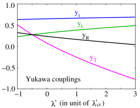
Figure 1: Yukawa couplings (ytsubscript𝑦𝑡y_{t}, yTsubscript𝑦𝑇y_{T}, yLsubscript𝑦𝐿y_{L}, yRsubscript𝑦𝑅y_{R}) as a function of λsuperscript𝜆\lambda^{\prime} (in unit of λcrsubscriptsuperscript𝜆𝑐𝑟\lambda^{\prime}_{cr}).

Since the mass of top quark mtsubscript𝑚𝑡m_{t} has already been measured precisely [9], there are four free parameters in the effective lagrangian of eq.(1). It is therefore possible to test the little higgs mechanism by measuring one more observable. This observable should be sensitive to λsuperscript𝜆\lambda^{\prime}, as pointed out in previous subsection. Since gauge interactions of the top partner depend only on sLsubscript𝑠𝐿s_{L}, we should focus on Yukawa interactions. In Fig. 1, we have shown coupling constants of Yukawa interactions (ytsubscript𝑦𝑡y_{t}, yTsubscript𝑦𝑇y_{T}, yLsubscript𝑦𝐿y_{L}, yRsubscript𝑦𝑅y_{R}) as functions of λsuperscript𝜆\lambda^{\prime} in unit of λcr(y32+yU2)/2subscriptsuperscript𝜆𝑐𝑟superscriptsubscript𝑦32superscriptsubscript𝑦𝑈22\lambda^{\prime}_{cr}\equiv-(y_{3}^{2}+y_{U}^{2})/2, so that λ=λcrsuperscript𝜆subscriptsuperscript𝜆𝑐𝑟\lambda^{\prime}=\lambda^{\prime}_{cr} corresponds to the prediction of the mechanism. Other model parameters are fixed to be those satisfying the conditions in eq.(14). It can be seen that the Yukawa coupling between top partners yTsubscript𝑦𝑇y_{T} is the most sensitive against the change of λsuperscript𝜆\lambda^{\prime} as expected. As a result, we should focus on physical quantities involving this Yukawa coupling.

3 Associate Productions

It can be easily imagined that top partner productions associated with a higgs boson enable us to explore the little higgs mechanism[10]. It is actually possible to measure the Yukawa coupling between top partners (yTsubscript𝑦𝑇y_{T}) simply by measuring cross sections of the processes with an appropriate center of mass energy. There are two higgs associated processes. One is the higgs production associating with a top quark and a top partner production (e+etT¯h&Tt¯h)e^{+}e^{-}\to t\bar{T}h~{}\&~{}T\bar{t}h), and another is the process associating with two top partners (e+eTT¯h)e^{+}e^{-}\to T\bar{T}h). At the former process, the center of mass energy smt+mT+mh𝑠subscript𝑚𝑡subscript𝑚𝑇subscript𝑚\sqrt{s}\geq m_{t}+m_{T}+m_{h} is, at least, required, which corresponds to about 700 GeV in our representative point. On the other hand, at the latter process, the center of mass energy should be higher than s2mT+mh𝑠2subscript𝑚𝑇subscript𝑚\sqrt{s}\geq 2m_{T}+m_{h}, which corresponds to 920 GeV in the representative point. In this section, we consider how the cross sections of these processes are sensitive against the change of the parameter λsuperscript𝜆\lambda^{\prime}, and discuss which process is suitable for the confirmation of the little higgs mechanism.

3.1 The e+etT¯h+Tt¯hsuperscript𝑒superscript𝑒𝑡¯𝑇𝑇¯𝑡e^{+}e^{-}\to t\bar{T}h+T\bar{t}h process

Refer to caption
Refer to caption
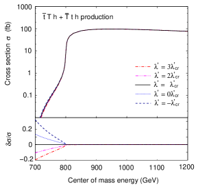
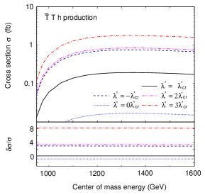
Figure 2: Cross sections for higgs associated productions e+etT¯h+Tt¯hsuperscript𝑒superscript𝑒𝑡¯𝑇𝑇¯𝑡e^{+}e^{-}\to t\bar{T}h+T\bar{t}h and e+eTT¯hsuperscript𝑒superscript𝑒𝑇¯𝑇e^{+}e^{-}\to T\bar{T}h as a function of center of mass energy. Results for several values of λsuperscript𝜆\lambda^{\prime} are shown.

We first consider the higgs production process associating with a top quark and a top partner. The sum of the cross sections, σ(e+etT¯h)+σ(e+eTt¯h)𝜎superscript𝑒superscript𝑒𝑡¯𝑇𝜎superscript𝑒superscript𝑒𝑇¯𝑡\sigma(e^{+}e^{-}\to t\bar{T}h)+\sigma(e^{+}e^{-}\to T\bar{t}h), are shown in Fig.2 (upper part of the left panel) as a function of center of mass energy with several choices of λsuperscript𝜆\lambda^{\prime}. Other model parameters to depict the figure are fixed according to the representative point in eq.(14). In order to see the sensitivity of the cross section against the change of λsuperscript𝜆\lambda^{\prime}, we also plot the deviation of the cross section from the one predicted by the little higgs mechanism, namely, δσ/σ[σ(λ)σ(λcr)]/σ(λcr)𝛿𝜎𝜎delimited-[]𝜎superscript𝜆𝜎subscriptsuperscript𝜆𝑐𝑟𝜎subscriptsuperscript𝜆𝑐𝑟\delta\sigma/\sigma\equiv[\sigma(\lambda^{\prime})-\sigma(\lambda^{\prime}_{cr})]/\sigma(\lambda^{\prime}_{cr}) (lower part of the left panel). It can be seen from the figure that the deviation becomes almost zero when the center of mass energy exceeds 800 GeV. This is because, with a center of mass energy higher than this value, two on-shell top partners can be produced, whose production cross section and branching ratio Tth𝑇𝑡T\to th are independent of the parameter λsuperscript𝜆\lambda^{\prime}, and this process dominates the associate production. On the other hand, the center of mass energy below 800 GeV, we can expect about 10% deviation. The cross section is, however, quite small below 800 GeV, which is about 0.1 fb. After all, the measurement of the Yukawa coupling λsuperscript𝜆\lambda^{\prime} turns out to be difficult in this associate production.

3.2 The e+eTT¯hsuperscript𝑒superscript𝑒𝑇¯𝑇e^{+}e^{-}\to T\bar{T}h process

Next, we consider the higgs production process associating with two top partners. As in the case of previous associate production, we show its production cross section σ(e+eTT¯h)𝜎superscript𝑒superscript𝑒𝑇¯𝑇\sigma(e^{+}e^{-}\rightarrow T\bar{T}h) in Fig.2 as a function of center of mass energy with various λsuperscript𝜆\lambda^{\prime} (upper part of the right panel). The deviation of the cross section from the little higgs prediction is also shown (lower part of the right panel). It can be seen from the figure that the cross section depends strongly on the value of λsuperscript𝜆\lambda^{\prime}, which enable us to explore the little higgs mechanism accurately using this association process, though the production cross section itself is not so large.

4 Threshold productions

We next consider top partner productions, e+eTT¯superscript𝑒superscript𝑒𝑇¯𝑇e^{+}e^{-}\to T\bar{T} and e+etT¯+Tt¯superscript𝑒superscript𝑒𝑡¯𝑇𝑇¯𝑡e^{+}e^{-}\to t\bar{T}+T\bar{t}, at the region of their threshold energies. Since the cross sections of these processes are significantly affected by the exchange of virtual higgs bosons due to the threshold singularity [11], the Yukawa coupling yTsubscript𝑦𝑇y_{T} is expected to be measured precisely. In this section, we consider how the cross sections are sensitive to the parameter λsuperscript𝜆\lambda^{\prime}.

4.1 Cross section formula

The cross section of top quark pair production at the e+esuperscript𝑒superscript𝑒e^{+}e^{-} collider (e+ett¯superscript𝑒superscript𝑒𝑡¯𝑡e^{+}e^{-}\to t\bar{t}) is known to have threshold singularities due to exchanges of soft gluons and higgs bosons between top quarks [11]. Productions of top partner are, in the same manner, expected to have the same singularities, which are quantitatively obtained by using a method of non-relativistic field theory [12]. Derivations of non-relativistic lagrangians for top partner productions and resultant cross section formulae are discussed in appendix C. For the case of top partner pair production (e+eTT¯superscript𝑒superscript𝑒𝑇¯𝑇e^{+}e^{-}\to T\bar{T}), the cross section at their threshold energy s2mTsimilar-to-or-equals𝑠2subscript𝑚𝑇\sqrt{s}\simeq 2m_{T} is obtained to be

σTT=[16QT2Qe2s2+12QTQevTves(smZ2)+6vT2(ve2+ae2)(smZ)2]Im[GTT(s2mT;𝟎,𝟎)],subscript𝜎𝑇𝑇delimited-[]16superscriptsubscript𝑄𝑇2superscriptsubscript𝑄𝑒2superscript𝑠212subscript𝑄𝑇subscript𝑄𝑒subscript𝑣𝑇subscript𝑣𝑒𝑠𝑠superscriptsubscript𝑚𝑍26superscriptsubscript𝑣𝑇2superscriptsubscript𝑣𝑒2superscriptsubscript𝑎𝑒2superscript𝑠subscript𝑚𝑍2Imdelimited-[]subscript𝐺𝑇𝑇𝑠2subscript𝑚𝑇00\displaystyle\sigma_{TT}=\left[\frac{16Q_{T}^{2}Q_{e}^{2}}{s^{2}}+\frac{12Q_{T}Q_{e}v_{T}v_{e}}{s(s-m_{Z}^{2})}+\frac{6v_{T}^{2}(v_{e}^{2}+a_{e}^{2})}{(s-m_{Z})^{2}}\right]{\rm Im}\left[G_{TT}(\sqrt{s}-2m_{T};{\bf 0},{\bf 0})\right], (15)

where QT=2e/3subscript𝑄𝑇2𝑒3Q_{T}=2e/3, vT=(g/cW)(2sW2/3+sL2/4)subscript𝑣𝑇𝑔subscript𝑐𝑊2superscriptsubscript𝑠𝑊23superscriptsubscript𝑠𝐿24v_{T}=(g/c_{W})(-2s_{W}^{2}/3+s_{L}^{2}/4), Qe=esubscript𝑄𝑒𝑒Q_{e}=-e, ve=(g/cW)(1/4+sW2)subscript𝑣𝑒𝑔subscript𝑐𝑊14superscriptsubscript𝑠𝑊2v_{e}=(g/c_{W})(-1/4+s_{W}^{2}), and ae=g/(4cW)subscript𝑎𝑒𝑔4subscript𝑐𝑊a_{e}=g/(4c_{W}). The mass of Z𝑍Z boson is denoted by mZsubscript𝑚𝑍m_{Z}. The green function GTT(E;𝐫,𝐫)subscript𝐺𝑇𝑇𝐸𝐫superscript𝐫G_{TT}(E;{\bf r},{\bf r}^{\prime}) in above formula satisfies the following Schro¨¨o\ddot{\rm o}dinger equation,

[𝐫2mT+VTT(𝐫)EiΓT2]GTT(E,𝐫,𝐫)=δ3(𝐫𝐫),delimited-[]superscriptsubscript𝐫2subscript𝑚𝑇subscript𝑉𝑇𝑇𝐫𝐸𝑖subscriptΓ𝑇2subscript𝐺𝑇𝑇𝐸𝐫superscript𝐫superscript𝛿3𝐫superscript𝐫\displaystyle\left[-\frac{\nabla_{\bf r}^{2}}{m_{T}}+V_{TT}({\bf r})-E-i\frac{\Gamma_{T}}{2}\right]G_{TT}(E,{\bf r},{\bf r}^{\prime})=\delta^{3}({\bf r}-{\bf r}^{\prime}), (16)

with appropriate boundary conditions [11]. Here, ΓTsubscriptΓ𝑇\Gamma_{T} is the total decay width of the top partner. All information of soft gluon and higgs exchanges between top partners are involved in the potential term VTT(𝐫)subscript𝑉𝑇𝑇𝐫V_{TT}({\bf r}), which is explicitly given by

VTT(𝐫)=1|𝐫|(4αs3+αTemh|𝐫|),subscript𝑉𝑇𝑇𝐫1𝐫4subscript𝛼𝑠3subscript𝛼𝑇superscript𝑒subscript𝑚𝐫\displaystyle V_{TT}({\bf r})=-\frac{1}{|{\bf r}|}\left(\frac{4\alpha_{s}}{3}+\alpha_{T}e^{-m_{h}|{\bf r}|}\right), (17)

where αs=gs2/(4π)subscript𝛼𝑠superscriptsubscript𝑔𝑠24𝜋\alpha_{s}=g_{s}^{2}/(4\pi) and αT=yT2/(4π)subscript𝛼𝑇superscriptsubscript𝑦𝑇24𝜋\alpha_{T}=y_{T}^{2}/(4\pi). In addition to QCD and Yukawa interactions, the electroweak interaction (the exchange of Z𝑍Z bosons or photons between top partners) also contributes to the potential. This effect is however negligible and not included in our calculations. Since one of the purposes of this article is to clarify the effectiveness of threshold productions to measure the Yukawa coupling yTsubscript𝑦𝑇y_{T}, we only consider the potential at the leading order calculation. In order to compare theoretical predictions with experimental results very precisely, we should include higher order contributions especially from QCD interactions [12]. Since those calculations are beyond the scope of this article and our conclusion about the effectiveness of threshold productions is expected not to be altered even if we include those effects222Including this effect alters the cross section by about 10 %. However, the degree of deviation of the cross section as we change λsuperscript𝜆\lambda^{\prime} is hardly affected., we omit the higher order contributions in our calculation.

On the other hand, for the case of top quark and top partner production, the cross section at the threshold energy region (smt+mTsimilar-to-or-equals𝑠subscript𝑚𝑡subscript𝑚𝑇\sqrt{s}\simeq m_{t}+m_{T}) turns out to be

σtT=12vtT2(ve2+ae2)(smZ2)2Im[GtT(smtmT,𝟎,𝟎)],subscript𝜎𝑡𝑇12superscriptsubscript𝑣𝑡𝑇2superscriptsubscript𝑣𝑒2superscriptsubscript𝑎𝑒2superscript𝑠superscriptsubscript𝑚𝑍22Imdelimited-[]subscript𝐺𝑡𝑇𝑠subscript𝑚𝑡subscript𝑚𝑇00\displaystyle\sigma_{tT}=\frac{12v_{tT}^{2}(v_{e}^{2}+a_{e}^{2})}{(s-m_{Z}^{2})^{2}}{\rm Im}\left[G_{tT}(\sqrt{s}-m_{t}-m_{T},{\bf 0},{\bf 0})\right], (18)

where vtT=gcLsL/(4sW)subscript𝑣𝑡𝑇𝑔subscript𝑐𝐿subscript𝑠𝐿4subscript𝑠𝑊v_{tT}=gc_{L}s_{L}/(4s_{W}). The green function GtT(E;𝐫,𝐫)subscript𝐺𝑡𝑇𝐸𝐫superscript𝐫G_{tT}(E;{\bf r},{\bf r}^{\prime}) satisfies the equation,

[𝐫22μtT+VtT(𝐫)EiΓtT2]GtT(E,𝐫,𝐫)=δ3(𝐫𝐫),delimited-[]superscriptsubscript𝐫22subscript𝜇𝑡𝑇subscript𝑉𝑡𝑇𝐫𝐸𝑖subscriptΓ𝑡𝑇2subscript𝐺𝑡𝑇𝐸𝐫superscript𝐫superscript𝛿3𝐫superscript𝐫\displaystyle\left[-\frac{\nabla_{\bf r}^{2}}{2\mu_{tT}}+V_{tT}({\bf r})-E-i\frac{\Gamma_{tT}}{2}\right]G_{tT}(E,{\bf r},{\bf r}^{\prime})=\delta^{3}({\bf r}-{\bf r}^{\prime}), (19)

where μtTsubscript𝜇𝑡𝑇\mu_{tT} is the inertial mass of top quark and top partner, μtT=mtmT/(mt+mT)subscript𝜇𝑡𝑇subscript𝑚𝑡subscript𝑚𝑇subscript𝑚𝑡subscript𝑚𝑇\mu_{tT}=m_{t}m_{T}/(m_{t}+m_{T}), while ΓtTsubscriptΓ𝑡𝑇\Gamma_{tT} is the averaged decay width of these particles, ΓtT=(Γt+ΓT)/2subscriptΓ𝑡𝑇subscriptΓ𝑡subscriptΓ𝑇2\Gamma_{tT}=(\Gamma_{t}+\Gamma_{T})/2 with ΓtsubscriptΓ𝑡\Gamma_{t} being the total decay width of the top quark. The potential VtT(𝐫)subscript𝑉𝑡𝑇𝐫V_{tT}({\bf r}) is given by

VtT(𝐫)=1|𝐫|(4αs3+ytyT4πemh|𝐫|).subscript𝑉𝑡𝑇𝐫1𝐫4subscript𝛼𝑠3subscript𝑦𝑡subscript𝑦𝑇4𝜋superscript𝑒subscript𝑚𝐫\displaystyle V_{tT}({\bf r})=-\frac{1}{|{\bf r}|}\left(\frac{4\alpha_{s}}{3}+\frac{y_{t}y_{T}}{4\pi}e^{-m_{h}|{\bf r}|}\right). (20)

Finally, we would like to add a comment on the scale of the strong coupling αssubscript𝛼𝑠\alpha_{s} which appears in the potential terms VTT(𝐫)subscript𝑉𝑇𝑇𝐫V_{TT}({\bf r}) and VTT(𝐫)subscript𝑉𝑇𝑇𝐫V_{TT}({\bf r}). The scale (μ𝜇\mu) is taken to be the solution of the following self-consistency equation of the coupling,

μ=m2×43×αs(run)(μ),𝜇𝑚243superscriptsubscript𝛼𝑠𝑟𝑢𝑛𝜇\displaystyle\mu=\frac{m}{2}\times\frac{4}{3}\times\alpha_{s}^{(run)}\left(\mu\right), (21)

where αs(run)(x)superscriptsubscript𝛼𝑠𝑟𝑢𝑛𝑥\alpha_{s}^{(run)}(x) is the running coupling of the strong interaction at the scale x𝑥x, and m𝑚m is the inertial mass of a two-body system, namely, m=mT/2𝑚subscript𝑚𝑇2m=m_{T}/2 for top partner pair production and m=mtmT/(mt+mT)𝑚subscript𝑚𝑡subscript𝑚𝑇subscript𝑚𝑡subscript𝑚𝑇m=m_{t}m_{T}/(m_{t}+m_{T}) for the production of top quark and top partner. This prescription is known to make higher order QCD corrections to the Coulomb potential small at the Bohr radius [13].

4.2 The e+eTT¯superscript𝑒superscript𝑒𝑇¯𝑇e^{+}e^{-}\to T\bar{T} process

Refer to caption
Refer to caption
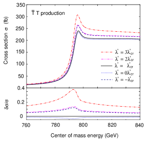
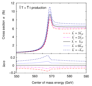
Figure 3: Cross sections for threshold productions e+eTT¯superscript𝑒superscript𝑒𝑇¯𝑇e^{+}e^{-}\to T\bar{T} and e+etT¯+Tt¯superscript𝑒superscript𝑒𝑡¯𝑇𝑇¯𝑡e^{+}e^{-}\to t\bar{T}+T\bar{t} as a function of center of mass energy. Results for several values of λsuperscript𝜆\lambda^{\prime} are shown.

We first consider the threshold production of top partner pair. The resultant cross section, which is obtained using the formula in eq.(15), is shown in the left panel of Fig. 3 with several choices of λsuperscript𝜆\lambda^{\prime}. In addition to the cross section, we also plot the deviation of the cross section from the prediction of the little higgs mechanism, δσ/σ𝛿𝜎𝜎\delta\sigma/\sigma, as in the case of higgs associated productions in previous section. It can be seen that the deviation becomes maximum at the peak of the cross section, which corresponds to the first bound state composed of top partners. Since the cross section is huge at the peak, which is about 250 fb-1, the Yukawa coupling yTsubscript𝑦𝑇y_{T} is expected to be measured precisely. It should be noticed that the potential VTT(𝐫)subscript𝑉𝑇𝑇𝐫V_{TT}({\bf r}) in eq.(17) does not depend on the sign of yTsubscript𝑦𝑇y_{T}, so that there is two-fold ambiguity in the determination of yTsubscript𝑦𝑇y_{T}, as can be seen in the figure. This ambiguity is easily resolved by investigating other production channels such as higgs associated productions.

4.3 The e+etT¯+Tt¯superscript𝑒superscript𝑒𝑡¯𝑇𝑇¯𝑡e^{+}e^{-}\to t\bar{T}+T\bar{t} process

We next consider the threshold production of a top quark and a top partner. Resultant cross section and its deviation from the little higgs prediction are plotted in the right panel of Fig. 3. As in the case of top partner pair production, the deviation is again maximized at the peak corresponding to the first bound state composed of top quark and top partner. Though the cross section is lower than that of the top partner pair production, which is of the order of 10 fb-1, it is still possible to measure λsuperscript𝜆\lambda^{\prime} precisely if the integrated luminosity is large enough. One of the advantages for the use of the process to test the little higgs mechanism is that the measurement of λsuperscript𝜆\lambda^{\prime} is possible even if the center of mass energy at the collision is not so large.

5 Testing the little higgs mechanism

We are now in position to discuss the capability of future linear colliders to test the little higgs mechanism. Testing the mechanism is, as already emphasized in section 2, equivalent to the measurement of the coupling constant λsuperscript𝜆\lambda^{\prime}. In this section, we therefore discuss how accurately the constant λsuperscript𝜆\lambda^{\prime} can be measured at collider experiments with the use of the processes discussed in previous sections.

5.1 The χ2superscript𝜒2\chi^{2} function

We focus on higgs associated production (e+eTT¯hsuperscript𝑒superscript𝑒𝑇¯𝑇e^{+}e^{-}\to T\bar{T}h) and threshold productions (e+eTT¯superscript𝑒superscript𝑒𝑇¯𝑇e^{+}e^{-}\to T\bar{T} and e+etT¯+Tt¯superscript𝑒superscript𝑒𝑡¯𝑇𝑇¯𝑡e^{+}e^{-}\to t\bar{T}+T\bar{t}), because the cross sections of these processes are very sensitive to the coupling constant λsuperscript𝜆\lambda^{\prime}. In order to maximize the capability of collider experiments for the measurement of λsuperscript𝜆\lambda^{\prime}, we set the center of mass energy to be 1000 GeV, 794 GeV and 568.4 GeV for TT¯h𝑇¯𝑇T\bar{T}h, TT¯𝑇¯𝑇T\bar{T} and tT¯+Tt¯𝑡¯𝑇𝑇¯𝑡t\bar{T}+T\bar{t} productions, respectively. On the other hand, the integrated luminosity is fixed to be eff=500subscripteff500{\cal L}_{\rm eff}=500 fb-1 in each process, where effsubscripteff{\cal L}_{\rm eff} is the effective luminosity defined by eff=×subscripteff{\cal L}_{\rm eff}={\cal E}\times{\cal L} with {\cal E} and {\cal L} being the efficiency factor and the original integrated luminosity.

The efficiency factor depends on the acceptance of collider detectors and kinematical cuts used to reduce backgrounds from SM processes, which is determined precisely when experiments start. Main backgrounds against the signal processes are from SM processes of top quark production. Since cross sections of the SM processes are not too large compared to those of signal processes, background reductions are expected to be performed efficiently by imposing appropriate kinematical cuts. The efficiency factor from background reductions can be estimated using Monte-Carlo simulations. In our calculation, however, we take the efficiency factor so that the effective luminosity becomes 500 fb-1 with simply assuming efficient background reductions. We remain the detailed calculation of the factor as a future problem.

With the use of the effective luminosity effsubscripteff{\cal L}_{\rm eff}, the χ2superscript𝜒2\chi^{2} function, which quantifies how accurately the λsuperscript𝜆\lambda^{\prime} measurement can be performed, is defined by

χ2(λ)[N(λ)N(λcr)]2N(λcr)=eff×[σ(λ)σ(λcr)]2σ(λcr),superscript𝜒2superscript𝜆superscriptdelimited-[]𝑁superscript𝜆𝑁subscriptsuperscript𝜆𝑐𝑟2𝑁subscriptsuperscript𝜆𝑐𝑟subscripteffsuperscriptdelimited-[]𝜎superscript𝜆𝜎subscriptsuperscript𝜆𝑐𝑟2𝜎subscriptsuperscript𝜆𝑐𝑟\displaystyle\chi^{2}(\lambda^{\prime})\equiv\frac{\left[N(\lambda^{\prime})-N(\lambda^{\prime}_{cr})\right]^{2}}{N(\lambda^{\prime}_{cr})}={\cal L}_{\rm eff}\times\frac{\left[\sigma(\lambda^{\prime})-\sigma(\lambda^{\prime}_{cr})\right]^{2}}{\sigma(\lambda^{\prime}_{cr})}, (22)

where N(λ)=effσ(λ)𝑁superscript𝜆subscripteff𝜎superscript𝜆N(\lambda^{\prime})={\cal L}_{\rm eff}\sigma(\lambda^{\prime}) is the number of the signal event with fixed λsuperscript𝜆\lambda^{\prime}, which will be obtained at collider experiments after imposing kinematical cuts and considering detector acceptances. Here, the value of λsuperscript𝜆\lambda^{\prime} predicted by the little higgs mechanism is denoted by λcr=(y32+yU2)/2subscriptsuperscript𝜆𝑐𝑟superscriptsubscript𝑦32superscriptsubscript𝑦𝑈22\lambda^{\prime}_{cr}=-(y_{3}^{2}+y_{U}^{2})/2. Other parameters to calculate the cross section σ𝜎\sigma is fixed according to a representative point mentioned in section 2.

5.2 Results
Refer to caption
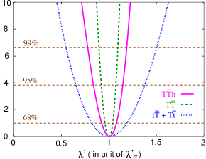
Figure 4: The χ2superscript𝜒2\chi^{2} distributions for e+eTT¯hsuperscript𝑒superscript𝑒𝑇¯𝑇e^{+}e^{-}\to T\bar{T}h, TT¯𝑇¯𝑇T\bar{T}, and tT¯+Tt¯𝑡¯𝑇𝑇¯𝑡t\bar{T}+T\bar{t} processes.

Resultant χ2superscript𝜒2\chi^{2} distributions for the higgs associated production (TT¯h𝑇¯𝑇T\bar{T}h) and threshold productions (TT¯𝑇¯𝑇T\bar{T} and tT¯+Tt¯𝑡¯𝑇𝑇¯𝑡t\bar{T}+T\bar{t}) are shown in Fig. 4, where the center of mass energy is fixed to be 1000 GeV, 794 GeV and 568.4 GeV, respectively. It can be seen that the coupling constant λsuperscript𝜆\lambda^{\prime} can be measured with 8% accuracy using the higgs associated production. If the center of mass energy is possible to be increased to 1350 GeV, the coupling λsuperscript𝜆\lambda^{\prime} can be measured with 4% accuracy using the same process.

On the other hand, it can be seen that the coupling constant λsuperscript𝜆\lambda^{\prime} can be measured with 4% accuracy using the threshold production of top partner pair production. In this case, the center of mass energy required for the measurement is smaller than that of the higgs associated production. Furthermore, using the threshold production of top quark and top partner, the coupling constant λsuperscript𝜆\lambda^{\prime} can be measured with 20% accuracy even if the center of mass energy is around 500 GeV.

6 Summary

We have studied the capability of future collider experiments to test the little higgs mechanism. The mechanism predicts a certain relation between coupling constants in the top sector of the little higgs scenario. The test of the mechanism is essentially equivalent to the measurement of the Yukawa coupling of the top partner, namely the coupling constant λsuperscript𝜆\lambda^{\prime}. It is therefore very important to investigate how accurately λsuperscript𝜆\lambda^{\prime} can be measured at the experiments. With the use of an appropriate representative point, we found that the coupling constant can be measured with a few percent accuracy using the higgs associated productions (e+eTT¯hsuperscript𝑒superscript𝑒𝑇¯𝑇e^{+}e^{-}\to T\bar{T}h) and the threshold production (e+eTT¯superscript𝑒superscript𝑒𝑇¯𝑇e^{+}e^{-}\to T\bar{T}), when the center of mass energy is 𝒪(1)𝒪1{\cal O}(1) TeV. On the other hand, using the threshold production (Tt¯+tT¯𝑇¯𝑡𝑡¯𝑇T\bar{t}+t\bar{T}), the measurement of λsuperscript𝜆\lambda^{\prime} is still possible with a few ten percent accuracy even if the center of mass energy is around 500 GeV. When the top partner is discovered at the LHC experiment, the processes emphasized in this article will be important to confirm whether the top partner is really the one predicted by the little higgs scenario or not.

Acknowledgments

This work is supported by Grant-in-Aid for Scientific research from the Ministry of Education, Science, Sports, and Culture (MEXT), Japan (Nos. 23740169, 22244031, 22244021 for S.M.), and also by World Premier International Research Center Initiative (WPI Initiative), MEXT, Japan.

Appendix A Effective lagrangian

A.1 Derivation

Dim. Operators
3 U¯LURsubscript¯𝑈𝐿subscript𝑈𝑅\bar{U}_{L}U_{R} U¯Lu3Rsubscript¯𝑈𝐿subscript𝑢3𝑅\bar{U}_{L}u_{3R}
4 U¯LULsubscript¯𝑈𝐿italic-D̸subscript𝑈𝐿\bar{U}_{L}\not{D}U_{L} U¯RURsubscript¯𝑈𝑅italic-D̸subscript𝑈𝑅\bar{U}_{R}\not{D}U_{R} Q¯3LHcURsubscript¯𝑄3𝐿superscript𝐻𝑐subscript𝑈𝑅\bar{Q}_{3L}H^{c}U_{R}
5 U¯LUR|H|2subscript¯𝑈𝐿subscript𝑈𝑅superscript𝐻2\bar{U}_{L}U_{R}|H|^{2} U¯L(Hc)Q3Lsubscript¯𝑈𝐿superscriptsuperscript𝐻𝑐italic-D̸subscript𝑄3𝐿\bar{U}_{L}(H^{c})^{\dagger}\not{D}Q_{3L} U¯Lσμνu3RBμνsubscript¯𝑈𝐿superscript𝜎𝜇𝜈subscript𝑢3𝑅subscript𝐵𝜇𝜈\bar{U}_{L}\sigma^{\mu\nu}u_{3R}B_{\mu\nu} U¯Lσμν(λa/2)u3RGμνasubscript¯𝑈𝐿superscript𝜎𝜇𝜈superscript𝜆𝑎2subscript𝑢3𝑅superscriptsubscript𝐺𝜇𝜈𝑎\bar{U}_{L}\sigma^{\mu\nu}(\lambda^{a}/2)u_{3R}G_{\mu\nu}^{a}
U¯Lu3R|H|2subscript¯𝑈𝐿subscript𝑢3𝑅superscript𝐻2\bar{U}_{L}u_{3R}|H|^{2} Q¯3LHcULsubscript¯𝑄3𝐿superscript𝐻𝑐italic-D̸subscript𝑈𝐿\bar{Q}_{3L}H^{c}\not{D}U_{L} U¯LσμνURBμνsubscript¯𝑈𝐿superscript𝜎𝜇𝜈subscript𝑈𝑅subscript𝐵𝜇𝜈\bar{U}_{L}\sigma^{\mu\nu}U_{R}B_{\mu\nu} U¯Lσμν(λa/2)URGμνasubscript¯𝑈𝐿superscript𝜎𝜇𝜈superscript𝜆𝑎2subscript𝑈𝑅superscriptsubscript𝐺𝜇𝜈𝑎\bar{U}_{L}\sigma^{\mu\nu}(\lambda^{a}/2)U_{R}G_{\mu\nu}^{a}
Table 2: Lorentz and gauge invariant operators including ULsubscript𝑈𝐿U_{L} and URsubscript𝑈𝑅U_{R}.

We first consider operators which are invariant under Lorentz and gauge symmetries of the SM. The operators including top partners ULsubscript𝑈𝐿U_{L} and URsubscript𝑈𝑅U_{R} are shown in Table 2 up to dimension five, where =Dμγμitalic-D̸subscript𝐷𝜇superscript𝛾𝜇\not{D}=D_{\mu}\gamma^{\mu} with Dμsubscript𝐷𝜇D_{\mu} being the covariant derivative, Gμνa(Bμν)superscriptsubscript𝐺𝜇𝜈𝑎subscript𝐵𝜇𝜈G_{\mu\nu}^{a}(B_{\mu\nu}) is the field strength tensor of gluon (hyper-charge gouge boson), σμν=i[γμ,γν]/2subscript𝜎𝜇𝜈𝑖subscript𝛾𝜇subscript𝛾𝜈2\sigma_{\mu\nu}=i[\gamma_{\mu},\gamma_{\nu}]/2, and λasuperscript𝜆𝑎\lambda^{a} is Gell-Mann matrix. Hermitian conjugates of the operators are not shown. Since the quantum number of u3Rsubscript𝑢3𝑅u_{3R} is exactly the same as that of URsubscript𝑈𝑅U_{R}, the bilinear operator U¯Lu3Rsubscript¯𝑈𝐿subscript𝑢3𝑅\bar{U}_{L}u_{3R} can be eliminated by an appropriate redefinition of URsubscript𝑈𝑅U_{R}. Dimension five operators U¯L(Hc)Q3Lsubscript¯𝑈𝐿superscriptsuperscript𝐻𝑐italic-D̸subscript𝑄3𝐿\bar{U}_{L}(H^{c})^{\dagger}\not{D}Q_{3L} and Q¯3LHcULsubscript¯𝑄3𝐿superscript𝐻𝑐italic-D̸subscript𝑈𝐿\bar{Q}_{3L}H^{c}\not{D}U_{L} are also eliminated by using the equations of motion. On the other hand, dipole-type operators U¯Lσμνu3RBμνsubscript¯𝑈𝐿superscript𝜎𝜇𝜈subscript𝑢3𝑅subscript𝐵𝜇𝜈\bar{U}_{L}\sigma^{\mu\nu}u_{3R}B_{\mu\nu}, U¯Lσμν(λa/2)u3RGμνasubscript¯𝑈𝐿superscript𝜎𝜇𝜈superscript𝜆𝑎2subscript𝑢3𝑅superscriptsubscript𝐺𝜇𝜈𝑎\bar{U}_{L}\sigma^{\mu\nu}(\lambda^{a}/2)u_{3R}G_{\mu\nu}^{a}, U¯LσμνURBμνsubscript¯𝑈𝐿superscript𝜎𝜇𝜈subscript𝑈𝑅subscript𝐵𝜇𝜈\bar{U}_{L}\sigma^{\mu\nu}U_{R}B_{\mu\nu} and U¯Lσμν(λa/2)URGμνasubscript¯𝑈𝐿superscript𝜎𝜇𝜈superscript𝜆𝑎2subscript𝑈𝑅superscriptsubscript𝐺𝜇𝜈𝑎\bar{U}_{L}\sigma^{\mu\nu}(\lambda^{a}/2)U_{R}G_{\mu\nu}^{a} do not contain higgs boson, so that they are suppressed by the cutoff scale Λsimilar-to-or-equalsΛabsent\Lambda\simeq 10 TeV. Furthermore, they are expected to appear radiatively from UV-completion theory of the little higgs scenario, and coefficients in front of the operators will be suppressed by 1-loop factor. The dipole-type operators are therefore negligible compared to other dimension five operators. The effective lagrangian including top partners is therefore given by

\displaystyle{\cal L} =\displaystyle= SM+U¯LiUL+U¯RiUR(mUU¯LUR+h.c.)\displaystyle{\cal L}_{\rm SM}+\bar{U}_{L}i\not{D}U_{L}+\bar{U}_{R}i\not{D}U_{R}-(m_{U}\bar{U}_{L}U_{R}+h.c.) (23)
\displaystyle- yUQ¯3LHcUR(λ/mU)U¯LUR|H|2(λ/mU)U¯Lu3R|H|2+h.c.,formulae-sequencesubscript𝑦𝑈subscript¯𝑄3𝐿superscript𝐻𝑐subscript𝑈𝑅superscript𝜆subscript𝑚𝑈subscript¯𝑈𝐿subscript𝑈𝑅superscript𝐻2𝜆subscript𝑚𝑈subscript¯𝑈𝐿subscript𝑢3𝑅superscript𝐻2𝑐\displaystyle y_{U}\bar{Q}_{3L}H^{c}U_{R}-(\lambda^{\prime}/m_{U})\bar{U}_{L}U_{R}|H|^{2}-(\lambda/m_{U})\bar{U}_{L}u_{3R}|H|^{2}+h.c.,

where SMsubscriptSM{\cal L}_{\rm SM} is the SM lagrangian. Parameters mUsubscript𝑚𝑈m_{U}, yUsubscript𝑦𝑈y_{U}, λ𝜆\lambda, and y3subscript𝑦3y_{3} (top yukawa in SMsubscriptSM{\cal L}_{\rm SM}) are taken to be real by appropriate redefinitions of Q3Lsubscript𝑄3𝐿Q_{3L}, u3Lsubscript𝑢3𝐿u_{3L}, ULsubscript𝑈𝐿U_{L}, and URsubscript𝑈𝑅U_{R}.

Using the effective lagrangian {\cal L}, quadratically divergent corrections to the higgs mass term from the top sector of the little higgs scenario turn out to be

δμt2(3y324π2+3yU24π2+3λ2π2)Λ2.similar-to-or-equals𝛿subscriptsuperscript𝜇2𝑡3superscriptsubscript𝑦324superscript𝜋23superscriptsubscript𝑦𝑈24superscript𝜋23superscript𝜆2superscript𝜋2superscriptΛ2\displaystyle\delta\mu^{2}_{t}\simeq\left(\frac{3y_{3}^{2}}{4\pi^{2}}+\frac{3y_{U}^{2}}{4\pi^{2}}+\frac{3\lambda^{\prime}}{2\pi^{2}}\right)\Lambda^{2}. (24)

Since the corrections should be vanished at 1-loop level because of the little higgs mechanism, we have a special relation among the parameters, 2λ=y32+yU22superscript𝜆superscriptsubscript𝑦32superscriptsubscript𝑦𝑈2-2\lambda^{\prime}=y_{3}^{2}+y_{U}^{2}.

A.2 Correspondence to specific little higgs models

For convenience we show correspondence between the effective lagrangian (23) and specific little higgs models written by a non-linear sigma model.

The littlest higgs model

The littlest higgs model is well-studied [17], so it is worth showing the correspondence of the effective lagrangian. This models is embeds the electroweak sector of the standard model in an SU(5)/SO(5)𝑆𝑈5𝑆𝑂5SU(5)/SO(5) non-linear sigma model. The global SU(5)𝑆𝑈5SU(5) is broken by gauging an [SU(2)×U(1)]2superscriptdelimited-[]𝑆𝑈2𝑈12[SU(2)\times U(1)]^{2} subgroup. So 4 of 14 Nambu-Goldstone bosons (NGBs) are absorbed by the broken gauge symmetry, and there are 10 NGBs. From a non-linear sigma model of the littlest higgs model, its top quark sector is given by

toplittlest=λ1fU¯Lu3Rλ2fU¯LUR+2λ1Q¯3LHcu3Rsuperscriptsubscript𝑡𝑜𝑝littlestsubscript𝜆1𝑓subscript¯𝑈𝐿superscriptsubscript𝑢3𝑅subscript𝜆2𝑓subscript¯𝑈𝐿superscriptsubscript𝑈𝑅2subscript𝜆1subscript¯𝑄3𝐿superscript𝐻𝑐superscriptsubscript𝑢3𝑅\displaystyle{\cal L}_{top}^{\rm littlest}=-\lambda_{1}f\bar{U}_{L}u_{3R}^{\prime}-\lambda_{2}f\bar{U}_{L}U_{R}^{\prime}+\sqrt{2}\lambda_{1}\bar{Q}_{3L}H^{c}u_{3R}^{\prime}
+λ1fU¯Lu3R|H|2+h.c. ,formulae-sequencesubscript𝜆1𝑓subscript¯𝑈𝐿superscriptsubscript𝑢3𝑅superscript𝐻2𝑐 \displaystyle+\frac{\lambda_{1}}{f}\bar{U}_{L}u_{3R}^{\prime}|H|^{2}+h.c.\mbox{ }, (25)

where f𝑓f is an energy scale at which SU(5)𝑆𝑈5SU(5) is spontanously broken down to SO(5)𝑆𝑂5SO(5). In order to remove one bilinear term, we define u3Rsubscript𝑢3𝑅u_{3R} and URsubscript𝑈𝑅U_{R} which are given by

(u3RUR)=(λ2λ12+λ22λ1λ12+λ22λ1λ12+λ22λ2λ12+λ22)(u3RUR),subscript𝑢3𝑅subscript𝑈𝑅subscript𝜆2superscriptsubscript𝜆12superscriptsubscript𝜆22subscript𝜆1superscriptsubscript𝜆12superscriptsubscript𝜆22subscript𝜆1superscriptsubscript𝜆12superscriptsubscript𝜆22subscript𝜆2superscriptsubscript𝜆12superscriptsubscript𝜆22superscriptsubscript𝑢3𝑅superscriptsubscript𝑈𝑅\displaystyle\left(\begin{array}[]{c}u_{3R}\\ U_{R}\end{array}\right)=\left(\begin{array}[]{cc}\frac{\lambda_{2}}{\sqrt{\lambda_{1}^{2}+\lambda_{2}^{2}}}&\frac{-\lambda_{1}}{\sqrt{\lambda_{1}^{2}+\lambda_{2}^{2}}}\\ \frac{\lambda_{1}}{\sqrt{\lambda_{1}^{2}+\lambda_{2}^{2}}}&\frac{\lambda_{2}}{\sqrt{\lambda_{1}^{2}+\lambda_{2}^{2}}}\end{array}\right)\left(\begin{array}[]{c}u_{3R}^{\prime}\\ U_{R}^{\prime}\end{array}\right), (32)

and then (25) becomes

toplittlest=λ^fU¯LUR+2λ1λ2λ^Q¯3LHcu3R+2λ12λ^Q¯3LHcURsuperscriptsubscript𝑡𝑜𝑝littlest^𝜆𝑓subscript¯𝑈𝐿subscript𝑈𝑅2subscript𝜆1subscript𝜆2^𝜆subscript¯𝑄3𝐿superscript𝐻𝑐subscript𝑢3𝑅2superscriptsubscript𝜆12^𝜆subscript¯𝑄3𝐿superscript𝐻𝑐subscript𝑈𝑅\displaystyle{\cal L}_{top}^{\rm littlest}=-\hat{\lambda}f\bar{U}_{L}U_{R}+\frac{\sqrt{2}\lambda_{1}\lambda_{2}}{\hat{\lambda}}\bar{Q}_{3L}H^{c}u_{3R}+\frac{\sqrt{2}\lambda_{1}^{2}}{\hat{\lambda}}\bar{Q}_{3L}H^{c}U_{R}
+λ1λ2λ^fU¯Lu3R|H|2+λ12λ^fU¯LUR|H|2+h.c. ,formulae-sequencesubscript𝜆1subscript𝜆2^𝜆𝑓subscript¯𝑈𝐿subscript𝑢3𝑅superscript𝐻2superscriptsubscript𝜆12^𝜆𝑓subscript¯𝑈𝐿subscript𝑈𝑅superscript𝐻2𝑐 \displaystyle+\frac{\lambda_{1}\lambda_{2}}{\hat{\lambda}f}\bar{U}_{L}u_{3R}|H|^{2}+\frac{\lambda_{1}^{2}}{\hat{\lambda}f}\bar{U}_{L}U_{R}|H|^{2}+h.c.\mbox{ }, (33)

where λ^=λ12+λ22^𝜆superscriptsubscript𝜆12superscriptsubscript𝜆22\hat{\lambda}=\sqrt{\lambda_{1}^{2}+\lambda_{2}^{2}}. We compare (33) to (1) and obtain following relations:

mU=λ^f,y3=2λ1λ2/λ^yU=2λ12/λ^,λ=λ1λ2λ=λ12 .subscript𝑚𝑈^𝜆𝑓subscript𝑦32subscript𝜆1subscript𝜆2^𝜆subscript𝑦𝑈2superscriptsubscript𝜆12^𝜆𝜆subscript𝜆1subscript𝜆2superscript𝜆superscriptsubscript𝜆12 \displaystyle\begin{array}[]{c}m_{U}=\hat{\lambda}f\\ \end{array},\begin{array}[]{c}y_{3}=-\sqrt{2}\lambda_{1}\lambda_{2}/\hat{\lambda}\\ y_{U}=-\sqrt{2}\lambda_{1}^{2}/\hat{\lambda}\end{array},\begin{array}[]{c}\lambda=-\lambda_{1}\lambda_{2}\\ \lambda^{\prime}=\lambda_{1}^{2}\end{array}\mbox{ }. (39)

These coefficients actually hold the relation (2).

The simplest lttle higgs model

We also consider the simplest little higgs model [18, 19], which has an [SU(3)×U(1)]2superscriptdelimited-[]𝑆𝑈3𝑈12[SU(3)\times U(1)]^{2} global symmetry spontaneously broken down to an [SU(2)×U(1)]2superscriptdelimited-[]𝑆𝑈2𝑈12[SU(2)\times U(1)]^{2} subgroup by two vacuum expectation values which are f1subscript𝑓1f_{1} and f2subscript𝑓2f_{2}. The diagonal subgroup of [SU(3)×U(1)]2superscriptdelimited-[]𝑆𝑈3𝑈12[SU(3)\times U(1)]^{2} is gauged, and 5 of 10 NGBs are absorbed by broken gauge fields. The remaining NGBs contains the higgs boson. The top quark sector of this model from a non-linear sigma model is given by

topsimple=λ1f1U¯LUR1λ1f2fQ¯3LHcUR1+λ1f222f1f2U¯LUR1|H|2superscriptsubscript𝑡𝑜𝑝simplesubscript𝜆1subscript𝑓1subscript¯𝑈𝐿subscript𝑈𝑅1subscript𝜆1subscript𝑓2𝑓subscript¯𝑄3𝐿superscript𝐻𝑐subscript𝑈𝑅1subscript𝜆1superscriptsubscript𝑓222subscript𝑓1superscript𝑓2subscript¯𝑈𝐿subscript𝑈𝑅1superscript𝐻2\displaystyle{\cal L}_{top}^{\rm simple}=-\lambda_{1}f_{1}\bar{U}_{L}U_{R1}-\frac{\lambda_{1}f_{2}}{f}\bar{Q}_{3L}H^{c}U_{R1}+\frac{\lambda_{1}f_{2}^{2}}{2f_{1}f^{2}}\bar{U}_{L}U_{R1}|H|^{2}
λ2f2U¯LUR2+λ2f1fQ¯3LHcUR2+λ2f122f2f2U¯LUR2|H|2+h.c. ,formulae-sequencesubscript𝜆2subscript𝑓2subscript¯𝑈𝐿subscript𝑈𝑅2subscript𝜆2subscript𝑓1𝑓subscript¯𝑄3𝐿superscript𝐻𝑐subscript𝑈𝑅2subscript𝜆2superscriptsubscript𝑓122subscript𝑓2superscript𝑓2subscript¯𝑈𝐿subscript𝑈𝑅2superscript𝐻2𝑐 \displaystyle-\lambda_{2}f_{2}\bar{U}_{L}U_{R2}+\frac{\lambda_{2}f_{1}}{f}\bar{Q}_{3L}H^{c}U_{R2}+\frac{\lambda_{2}f_{1}^{2}}{2f_{2}f^{2}}\bar{U}_{L}U_{R2}|H|^{2}+h.c.\mbox{ }, (40)

where f=f12+f22𝑓superscriptsubscript𝑓12superscriptsubscript𝑓22f=\sqrt{f_{1}^{2}+f_{2}^{2}}. Redefine the right-handed top quarks as in the previous model in the following way

(URu3R)=(λ1f1Mλ2f2Mλ2f2Mλ1f1M)(UR1UR2),subscript𝑈𝑅subscript𝑢3𝑅subscript𝜆1subscript𝑓1𝑀subscript𝜆2subscript𝑓2𝑀subscript𝜆2subscript𝑓2𝑀subscript𝜆1subscript𝑓1𝑀subscript𝑈𝑅1subscript𝑈𝑅2\displaystyle\left(\begin{array}[]{c}U_{R}\\ u_{3R}\end{array}\right)=\left(\begin{array}[]{cc}\frac{\lambda_{1}f_{1}}{M}&\frac{\lambda_{2}f_{2}}{M}\\ \frac{-\lambda_{2}f_{2}}{M}&\frac{\lambda_{1}f_{1}}{M}\end{array}\right)\left(\begin{array}[]{c}U_{R1}\\ U_{R2}\end{array}\right), (47)

where M=λ12f12+λ22f22𝑀superscriptsubscript𝜆12superscriptsubscript𝑓12superscriptsubscript𝜆22superscriptsubscript𝑓22M=\sqrt{\lambda_{1}^{2}f_{1}^{2}+\lambda_{2}^{2}f_{2}^{2}}. Then the top sector becomes

topsimplesuperscriptsubscript𝑡𝑜𝑝simple\displaystyle{\cal L}_{top}^{\rm simple} =\displaystyle= MU¯LUR𝑀subscript¯𝑈𝐿subscript𝑈𝑅\displaystyle-M\bar{U}_{L}U_{R} (48)
+\displaystyle+ λ1λ2(f12+f22)fMQ¯3LHcu3Rf1f2(λ12λ22)fMQ¯3LHcURsubscript𝜆1subscript𝜆2superscriptsubscript𝑓12superscriptsubscript𝑓22𝑓𝑀subscript¯𝑄3𝐿superscript𝐻𝑐subscript𝑢3𝑅subscript𝑓1subscript𝑓2superscriptsubscript𝜆12superscriptsubscript𝜆22𝑓𝑀subscript¯𝑄3𝐿superscript𝐻𝑐subscript𝑈𝑅\displaystyle\frac{\lambda_{1}\lambda_{2}(f_{1}^{2}+f_{2}^{2})}{fM}\bar{Q}_{3L}H^{c}u_{3R}-\frac{f_{1}f_{2}(\lambda_{1}^{2}-\lambda_{2}^{2})}{fM}\bar{Q}_{3L}H^{c}U_{R}
+\displaystyle+ λ1λ22f2M(f13f2f23f1)U¯Lu3R|H|2+λ12f22+λ22f122f2MU¯LUR|H|2subscript𝜆1subscript𝜆22superscript𝑓2𝑀superscriptsubscript𝑓13subscript𝑓2superscriptsubscript𝑓23subscript𝑓1subscript¯𝑈𝐿subscript𝑢3𝑅superscript𝐻2superscriptsubscript𝜆12superscriptsubscript𝑓22superscriptsubscript𝜆22superscriptsubscript𝑓122superscript𝑓2𝑀subscript¯𝑈𝐿subscript𝑈𝑅superscript𝐻2\displaystyle\frac{\lambda_{1}\lambda_{2}}{2f^{2}M}\left(\frac{f_{1}^{3}}{f_{2}}-\frac{f_{2}^{3}}{f_{1}}\right)\bar{U}_{L}u_{3R}|H|^{2}+\frac{\lambda_{1}^{2}f_{2}^{2}+\lambda_{2}^{2}f_{1}^{2}}{2f^{2}M}\bar{U}_{L}U_{R}|H|^{2}
+\displaystyle+ h.c.formulae-sequence𝑐\displaystyle h.c.\mbox{}

As a result, we have

mU=M,y3=λ1λ2(f12+f22)fMyU=f1f2(λ12λ22)fM,λ=λ1λ22f2(f13f2f23f1)λ=λ12f22+λ22f122f2 .subscript𝑚𝑈𝑀subscript𝑦3subscript𝜆1subscript𝜆2superscriptsubscript𝑓12superscriptsubscript𝑓22𝑓𝑀subscript𝑦𝑈subscript𝑓1subscript𝑓2superscriptsubscript𝜆12superscriptsubscript𝜆22𝑓𝑀𝜆subscript𝜆1subscript𝜆22superscript𝑓2superscriptsubscript𝑓13subscript𝑓2superscriptsubscript𝑓23subscript𝑓1superscript𝜆superscriptsubscript𝜆12superscriptsubscript𝑓22superscriptsubscript𝜆22superscriptsubscript𝑓122superscript𝑓2 \displaystyle\begin{array}[]{c}m_{U}=M\\ \end{array},\begin{array}[]{c}y_{3}=-\frac{\lambda_{1}\lambda_{2}(f_{1}^{2}+f_{2}^{2})}{fM}\\ y_{U}=\frac{f_{1}f_{2}(\lambda_{1}^{2}-\lambda_{2}^{2})}{fM}\end{array},\begin{array}[]{c}\lambda=-\frac{\lambda_{1}\lambda_{2}}{2f^{2}}\left(\frac{f_{1}^{3}}{f_{2}}-\frac{f_{2}^{3}}{f_{1}}\right)\\ \lambda^{\prime}=-\frac{\lambda_{1}^{2}f_{2}^{2}+\lambda_{2}^{2}f_{1}^{2}}{2f^{2}}\end{array}\mbox{ }. (54)

These also satisfy the relation (2).

Appendix B Representative point

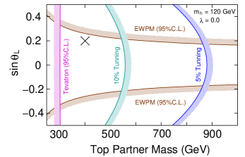
The representative point used in our analysis has been chosen so that it is consistent with current experimental data and also attractive from the viewpoint of the naturalness to keep the higgs mass (mhsubscript𝑚m_{h}) at the electroweak scale. The most stringent constraints on the parameter sinθLsubscript𝜃𝐿\sin\theta_{L} comes from the electroweak precession tests. Contributions to S𝑆S, T𝑇T, and U𝑈U parameters [14] from the top partner have already been calculated in Ref. [15]. On the other hand, hadron collider experiments give the lower bound on the mass of top partner (mTsubscript𝑚𝑇m_{T}). Currently, the CDF collaboration at the Tevatron experiment gives the stringent bound on mTsubscript𝑚𝑇m_{T} thorough the semi-leptonic mode of the process, pp¯TT¯bbWW𝑝¯𝑝𝑇¯𝑇𝑏𝑏𝑊𝑊p\bar{p}\to T\bar{T}\to bbWW~{}[16]. The upper bound on mTsubscript𝑚𝑇m_{T} is obtained from the viewpoint of the naturalness. Though quadratically divergent corrections to mhsubscript𝑚m_{h} are cancelled at 1-loop level, logarithmic corrections still remain at this level. Too large contributions therefore cause a fine-tuning to keep mhsubscript𝑚m_{h} at the electroweak scale [17]. Logarithmic contributions from the top sector are given by

δμt2=yt23mU28π2ln(Λ2mU2)3mT24π2mt2v2ln(Λ2mT2),𝛿superscriptsubscript𝜇𝑡2superscriptsubscript𝑦𝑡23superscriptsubscript𝑚𝑈28superscript𝜋2superscriptΛ2superscriptsubscript𝑚𝑈2similar-to-or-equals3superscriptsubscript𝑚𝑇24superscript𝜋2superscriptsubscript𝑚𝑡2superscript𝑣2superscriptΛ2superscriptsubscript𝑚𝑇2\displaystyle\delta\mu_{t}^{2}=y_{t}^{2}\frac{3m_{U}^{2}}{8\pi^{2}}\ln\left(\frac{\Lambda^{2}}{m_{U}^{2}}\right)\simeq\frac{3m_{T}^{2}}{4\pi^{2}}\frac{m_{t}^{2}}{v^{2}}\ln\left(\frac{\Lambda^{2}}{m_{T}^{2}}\right), (55)

with imposing the relation in eq.(2). Here, Λsimilar-to-or-equalsΛabsent\Lambda\simeq 10 TeV is the cutoff scale of the little higgs scenario. The level of the fine-tuning is parameterized by Fmh2/(2δμt2)𝐹superscriptsubscript𝑚22𝛿superscriptsubscript𝜇𝑡2F\equiv m_{h}^{2}/(2\delta\mu_{t}^{2}).

Refer to caption
Figure 5: Constraints on the model parameters and the representative point.

These constraints on the (mT,sinθL)subscript𝑚𝑇subscript𝜃𝐿(m_{T},\sin\theta_{L})-plane are summarized in Fig. 5, where λsuperscript𝜆\lambda^{\prime} is set so that it satisfies the little higgs relation in eq.(2). The representative point is denoted by the cross. It can be seen that the point satisfies the experimental constraints and the level of fine-tuning is less than 10% (F0.1𝐹0.1F\leq 0.1).

Appendix C Non-relativistic lagrangian

Derivation of the non-relativistic lagrangian for threshold productions is considered in this appendix. For concrete discussion, we consider the process of top partner pair production at the threshold energy s2mTsimilar-to-or-equals𝑠2subscript𝑚𝑇\sqrt{s}\simeq 2m_{T}. With the use of the effective lagrangian in eq.(23), interactions relevant to the threshold production are

\displaystyle{\cal L} =\displaystyle= T¯(i∂̸mT)T12h(2+mh2)h+12Gμa2Gμa+12Aμ2Aμ¯𝑇𝑖not-partial-differentialsubscript𝑚𝑇𝑇12superscript2superscriptsubscript𝑚212superscriptsubscript𝐺𝜇𝑎superscript2superscript𝐺𝜇𝑎12subscript𝐴𝜇superscript2superscript𝐴𝜇\displaystyle\bar{T}(i\not{\partial}-m_{T})T-\frac{1}{2}h(\partial^{2}+m_{h}^{2})h+\frac{1}{2}G_{\mu}^{a}\partial^{2}G^{\mu a}+\frac{1}{2}A_{\mu}\partial^{2}A^{\mu} (56)
+e¯i∂̸eyTT¯ThgsT¯TQTT¯TvTT¯T¯𝑒𝑖not-partial-differential𝑒subscript𝑦𝑇¯𝑇𝑇subscript𝑔𝑠¯𝑇italic-G̸𝑇subscript𝑄𝑇¯𝑇italic-A̸𝑇subscript𝑣𝑇¯𝑇italic-Z̸𝑇\displaystyle+\bar{e}i\not{\partial}e-y_{T}\bar{T}Th-g_{s}\bar{T}\not{G}T-Q_{T}\bar{T}\not{A}T-v_{T}\bar{T}\not{Z}T
+12Zμ[gμν(2+mZ2)μν]ZνQee¯ee¯(ve+aeγ5)e,12subscript𝑍𝜇delimited-[]superscript𝑔𝜇𝜈superscript2superscriptsubscript𝑚𝑍2superscript𝜇superscript𝜈subscript𝑍𝜈subscript𝑄𝑒¯𝑒italic-A̸𝑒¯𝑒italic-Z̸subscript𝑣𝑒subscript𝑎𝑒superscript𝛾5𝑒\displaystyle+\frac{1}{2}Z_{\mu}\left[g^{\mu\nu}(\partial^{2}+m_{Z}^{2})-\partial^{\mu}\partial^{\nu}\right]Z_{\nu}-Q_{e}\bar{e}\not{A}e-\bar{e}\not{Z}(v_{e}+a_{e}\gamma^{5})e,

where e𝑒e is the electron field. Unitarity (Feynman) gauge is adopted for Z𝑍Z boson (photon and gluon). After integrating higgs and gluon fields out from the lagrangian and expanding the top partner field T𝑇T in terms of its velocity (non-relativistic expansion), namely, T(eimTtη+ieimTtσχ/2mT,eimTtχieimTtση/2mT)Tsimilar-to-or-equals𝑇superscriptsuperscript𝑒𝑖subscript𝑚𝑇𝑡𝜂𝑖superscript𝑒𝑖subscript𝑚𝑇𝑡𝜎𝜒2subscript𝑚𝑇superscript𝑒𝑖subscript𝑚𝑇𝑡𝜒𝑖superscript𝑒𝑖subscript𝑚𝑇𝑡𝜎𝜂2subscript𝑚𝑇𝑇T\simeq(e^{-im_{T}t}\eta+ie^{im_{T}t}\nabla\cdot\sigma\chi/2m_{T},~{}e^{im_{T}t}\chi-ie^{-im_{T}t}\nabla\cdot\sigma\eta/2m_{T})^{T}, the effective action for non-relativistic fields η𝜂\eta and χ𝜒\chi is obtained as

Seffsubscript𝑆eff\displaystyle S_{\rm eff} =\displaystyle= d4x[η(it+22mT+iΓT2)η+χ(it22mTiΓT2)χ]superscript𝑑4𝑥delimited-[]superscript𝜂𝑖subscript𝑡superscript22subscript𝑚𝑇𝑖subscriptΓ𝑇2𝜂superscript𝜒𝑖subscript𝑡superscript22subscript𝑚𝑇𝑖subscriptΓ𝑇2𝜒\displaystyle\int d^{4}x\left[\eta^{\dagger}\left(i\partial_{t}+\frac{\nabla^{2}}{2m_{T}}+i\frac{\Gamma_{T}}{2}\right)\eta+\chi^{\dagger}\left(i\partial_{t}-\frac{\nabla^{2}}{2m_{T}}-i\frac{\Gamma_{T}}{2}\right)\chi\right] (57)
+\displaystyle+ d4xd4yδ(x0y0)VTT(𝐱𝐲)6[η(x)σiχ(y)][χ(y)σiη(x)]superscript𝑑4𝑥superscript𝑑4𝑦𝛿superscript𝑥0superscript𝑦0subscript𝑉𝑇𝑇𝐱𝐲6delimited-[]superscript𝜂𝑥superscript𝜎𝑖𝜒𝑦delimited-[]superscript𝜒𝑦superscript𝜎𝑖𝜂𝑥\displaystyle\int d^{4}x~{}d^{4}y~{}\delta(x^{0}-y^{0})\frac{V_{TT}({\bf x}-{\bf y})}{6}\left[\eta^{\dagger}(x)\sigma^{i}\chi(y)\right]\left[\chi^{\dagger}(y)\sigma^{i}\eta(x)\right]
+\displaystyle+ d4x[QTAi(e2imTησiχ+h.c.)+vTZi(e2imTησiχ+h.c.)]\displaystyle\int d^{4}x\left[Q_{T}A^{i}(e^{2im_{T}}\eta^{\dagger}\sigma^{i}\chi+h.c.)+v_{T}Z^{i}(e^{2im_{T}}\eta^{\dagger}\sigma^{i}\chi+h.c.)\right]
+\displaystyle+ d4x[e¯i∂̸eQee¯ee¯(ve+aeγ5)e],superscript𝑑4𝑥delimited-[]¯𝑒𝑖not-partial-differential𝑒subscript𝑄𝑒¯𝑒italic-A̸𝑒¯𝑒italic-Z̸subscript𝑣𝑒subscript𝑎𝑒superscript𝛾5𝑒\displaystyle\int d^{4}x\left[\bar{e}i\not{\partial}e-Q_{e}\bar{e}\not{A}e-\bar{e}\not{Z}(v_{e}+a_{e}\gamma^{5})e\right],

where the superscript ’i𝑖i’ runs from one to three, σisuperscript𝜎𝑖\sigma^{i} is the Pauli matrix, and ΓTsubscriptΓ𝑇\Gamma_{T} is the total decay width of the top partner. The potential VTT(𝐫)subscript𝑉𝑇𝑇𝐫V_{TT}({\bf r}) has already been defined in eq.(17). In addition to the terms in above action (57), we also have another potential terms such as the one composing spin-zero state ([η(x)χ(y)]proportional-toabsentdelimited-[]superscript𝜂𝑥𝜒𝑦\propto[\eta^{\dagger}(x)\chi(y)]) and those composing color octet states ([η(x)λaσiχ(y)]proportional-toabsentdelimited-[]superscript𝜂𝑥superscript𝜆𝑎superscript𝜎𝑖𝜒𝑦\propto[\eta^{\dagger}(x)\lambda^{a}\sigma^{i}\chi(y)] & [η(x)λaχ(y)]delimited-[]superscript𝜂𝑥superscript𝜆𝑎𝜒𝑦[\eta^{\dagger}(x)\lambda^{a}\chi(y)]), where λasuperscript𝜆𝑎\lambda^{a} is the Gell-Mann matrix. Since these states are never produced at high energy e±superscript𝑒plus-or-minuse^{\pm} collisions, we have dropped these terms from the effective action. In order to calculate the cross section at the threshold energy, it is convenient to introduce the auxiliary fields σtisubscriptsuperscript𝜎𝑖𝑡\sigma^{i}_{t} and σtisubscriptsuperscript𝜎𝑖𝑡\sigma^{i\dagger}_{t} by inserting following identities into the action,

1=𝒟σi𝒟siexp[i2d3xd3y𝑑tσti(𝐱,𝐲){sti(𝐲,𝐱)η(𝐱,t)σiχ(𝐲,t)3}],1𝒟superscript𝜎𝑖𝒟superscript𝑠𝑖𝑖2superscript𝑑3𝑥superscript𝑑3𝑦differential-d𝑡subscriptsuperscript𝜎𝑖𝑡𝐱𝐲subscriptsuperscript𝑠𝑖𝑡𝐲𝐱superscript𝜂𝐱𝑡superscript𝜎𝑖𝜒𝐲𝑡3\displaystyle 1=\int{\cal D}\sigma^{i}{\cal D}s^{i\dagger}\exp\left[\frac{i}{2}\int d^{3}x~{}d^{3}y~{}dt~{}\sigma^{i}_{t}({\bf x},{\bf y})\left\{s^{i\dagger}_{t}({\bf y},{\bf x})-\frac{\eta^{\dagger}({\bf x},t)\sigma^{i}\chi({\bf y},t)}{\sqrt{3}}\right\}\right],
1=𝒟σi𝒟siexp[i2d3xd3y𝑑tσti(𝐱,𝐲){sti(𝐲,𝐱)χ(𝐲,t)σiη(𝐱,t)3}].1𝒟superscript𝜎𝑖𝒟superscript𝑠𝑖𝑖2superscript𝑑3𝑥superscript𝑑3𝑦differential-d𝑡subscriptsuperscript𝜎𝑖𝑡𝐱𝐲subscriptsuperscript𝑠𝑖𝑡𝐲𝐱superscript𝜒𝐲𝑡superscript𝜎𝑖𝜂𝐱𝑡3\displaystyle 1=\int{\cal D}\sigma^{i\dagger}{\cal D}s^{i}\exp\left[\frac{i}{2}\int d^{3}x~{}d^{3}y~{}dt~{}\sigma^{i\dagger}_{t}({\bf x},{\bf y})\left\{s^{i}_{t}({\bf y},{\bf x})-\frac{\chi^{\dagger}({\bf y},t)\sigma^{i}\eta({\bf x},t)}{\sqrt{3}}\right\}\right]. (58)

Here, we integrate all fields out except the auxiliary fields (σtisubscriptsuperscript𝜎𝑖𝑡\sigma^{i}_{t} and σtisubscriptsuperscript𝜎𝑖𝑡\sigma^{i\dagger}_{t}) from the effective action in eq.(57), and canonically normalize σtisubscriptsuperscript𝜎𝑖𝑡\sigma^{i}_{t} and σtisubscriptsuperscript𝜎𝑖𝑡\sigma^{i\dagger}_{t} as

ϕTTi(𝐫,R)=12VTT(𝐫)[σti(𝐱,𝐲)+23e2imTtδ(𝐱𝐲){vTZi(x)+QTAi(x)}],superscriptsubscriptitalic-ϕ𝑇𝑇𝑖𝐫𝑅12subscript𝑉𝑇𝑇𝐫delimited-[]subscriptsuperscript𝜎𝑖𝑡𝐱𝐲23superscript𝑒2𝑖subscript𝑚𝑇𝑡𝛿𝐱𝐲subscript𝑣𝑇superscript𝑍𝑖𝑥subscript𝑄𝑇superscript𝐴𝑖𝑥\displaystyle\phi_{TT}^{i}({\bf r},R)=\frac{1}{\sqrt{2}V_{TT}({\bf r})}\left[\sigma^{i}_{t}({\bf x},{\bf y})+2\sqrt{3}e^{2im_{T}t}\delta({\bf x}-{\bf y})\left\{v_{T}Z^{i}(x)+Q_{T}A^{i}(x)\right\}\right], (59)

where variables 𝐫𝐫{\bf r}, 𝐑𝐑{\bf R} and R0superscript𝑅0R^{0} are defined by 𝐫=𝐱𝐲𝐫𝐱𝐲{\bf r}={\bf x}-{\bf y} and 𝐑=(𝐱+𝐲)/2𝐑𝐱𝐲2{\bf R}=({\bf x}+{\bf y})/2 and R0=tsuperscript𝑅0𝑡R^{0}=t, respectively. We then obtain the non-relativistic lagrangian directly used to calculate the cross section for the threshold production of the top partner pair,

SNR(TT)superscriptsubscript𝑆NR𝑇𝑇\displaystyle S_{\rm NR}^{(TT)} =\displaystyle= d4Rd3rϕTTi(𝐫,R)[iR0+𝐑24mT+𝐫2mTTVTT(𝐫)+iΓT]ϕTTi(𝐫,R),superscript𝑑4𝑅superscript𝑑3𝑟superscriptsubscriptitalic-ϕ𝑇𝑇𝑖𝐫𝑅delimited-[]𝑖subscriptsuperscript𝑅0subscriptsuperscript2𝐑4subscript𝑚𝑇subscriptsuperscript2𝐫subscript𝑚𝑇𝑇subscript𝑉𝑇𝑇𝐫𝑖subscriptΓ𝑇superscriptsubscriptitalic-ϕ𝑇𝑇𝑖𝐫𝑅\displaystyle\int d^{4}R~{}d^{3}r~{}\phi_{TT}^{i\dagger}({\bf r},R)\left[i\partial_{R^{0}}+\frac{\nabla^{2}_{\bf R}}{4m_{T}}+\frac{\nabla^{2}_{\bf r}}{m_{T}T}-V_{TT}({\bf r})+i\Gamma_{T}\right]\phi_{TT}^{i}({\bf r},R), (60)
\displaystyle- d4R[6e2imTR0ϕTTi(𝟎,R){vTZi(R)+QTAi(R)}+h.c.]\displaystyle\int d^{4}R\left[\sqrt{6}e^{2im_{T}R^{0}}\phi_{TT}^{i\dagger}({\bf 0},R)\left\{v_{T}Z^{i}(R)+Q_{T}A^{i}(R)\right\}+h.c.\right]
+\displaystyle+ d4x[e¯i∂̸eQee¯ee¯(ve+aeγ5)e].superscript𝑑4𝑥delimited-[]¯𝑒𝑖not-partial-differential𝑒subscript𝑄𝑒¯𝑒italic-A̸𝑒¯𝑒italic-Z̸subscript𝑣𝑒subscript𝑎𝑒superscript𝛾5𝑒\displaystyle\int d^{4}x\left[\bar{e}i\not{\partial}e-Q_{e}\bar{e}\not{A}e-\bar{e}\not{Z}(v_{e}+a_{e}\gamma^{5})e\right].

The fields ϕTTisubscriptsuperscriptitalic-ϕ𝑖𝑇𝑇\phi^{i}_{TT} and ϕTTisubscriptsuperscriptitalic-ϕ𝑖𝑇𝑇\phi^{i\dagger}_{TT} are describing the annihilation and creation of top partner pair, respectively. It can be seen that the effect of the threshold singularity is involved in the first term of the action with the form of the Schro¨¨o\ddot{\rm o}dinger equation. The non-relativistic action for the case of top quark and top partner production can be obtained in the same procedure of top partner pair production.

Cross section formulae for threshold productions are obtained by using the optical theorem, which is related to the calculation of the forward scattering amplitude. The cross section of the top partner pair production is, for instance, given by

σTT=1sIm[(e+eTT¯e+e)].subscript𝜎𝑇𝑇1𝑠Imdelimited-[]superscript𝑒superscript𝑒𝑇¯𝑇superscript𝑒superscript𝑒\displaystyle\sigma_{TT}=\frac{1}{s}{\rm Im}\left[{\cal M}(e^{+}e^{-}\to T\bar{T}\to e^{+}e^{-})\right]. (61)

Amplitude {\cal M} is calculated using above non-relativistic action, and eventually obtain the cross section formula in eq.(15). It is worth notifying that the solution of Schro¨¨o\ddot{\rm o}dinger equation in eq.(16) is required to calculate {\cal M} quantitatively, as already mentioned in section 4. Here, the green function GTT(E;𝐫,𝐫)subscript𝐺𝑇𝑇𝐸𝐫superscript𝐫G_{TT}(E;{\bf r},{\bf r}^{\prime}) in this equation is nothing but the Fourier transform of the following two-point function,

GTT(E,𝐫,𝐫)=id4R0|T[ϕTTi(𝐫,R)ϕTTi(𝐫,R)]|0eiE(RR),subscript𝐺𝑇𝑇𝐸𝐫superscript𝐫𝑖superscript𝑑4𝑅quantum-operator-product0𝑇delimited-[]superscriptsubscriptitalic-ϕ𝑇𝑇𝑖𝐫𝑅superscriptsubscriptitalic-ϕ𝑇𝑇𝑖superscript𝐫superscript𝑅0superscript𝑒𝑖𝐸𝑅superscript𝑅\displaystyle G_{TT}(E,{\bf r},{\bf r}^{\prime})=i\int d^{4}R\langle 0|T\left[\phi_{TT}^{i}({\bf r},R)\phi_{TT}^{i\dagger}({\bf r}^{\prime},R^{\prime})\right]|0\rangle e^{iE(R-R^{\prime})}, (62)

where 0|T[]|0quantum-operator-product0𝑇delimited-[]0\langle 0|T[\cdots]|0\rangle is the vacuum expectation value of the time-ordered product.

References

  • [1] For recent analysis, see R. Barbieri, A. Pomarol, R. Rattazzi, A. Strumia, Nucl. Phys.  B703, 127-146 (2004); Z. Han, W. Skiba, Phys. Rev.  D71, 075009 (2005).
  • [2] N. Arkani-Hamed, A. G. Cohen, H. Georgi, Phys. Lett.  B513, 232-240 (2001), and, for review, see M. Perelstein, Prog. Part. Nucl. Phys.  58, 247 (2007).
  • [3] G. Azuelos et al., Eur. Phys. J.  C 39S2, 13 (2005); J. Hubisz, P. Meade, Phys. Rev.  D71, 035016 (2005); J. A. Aguilar-Saavedra, Phys. Lett.  B 625, 234 (2005) [Erratum-ibid.  B 633, 792 (2006)]; T. Han, H. E. Logan, L. -T. Wang, JHEP 0601, 099 (2006); J. A. Aguilar-Saavedra, JHEP 0612, 033 (2006); K. Cheung, C. S. Kim, K. Y. Lee, J. Song, Phys. Rev.  D74, 115013 (2006); W. Skiba, D. Tucker-Smith, Phys. Rev.  D75, 115010 (2007); S. Matsumoto, T. Moroi, K. Tobe, Phys. Rev.  D78, 055018 (2008); G. Dissertori, E. Furlan, F. Moortgat, P. Nef, JHEP 1009, 019 (2010); W. S.  Cho, K. Harigaya, S. Matsumoto, M. M. Nojiri, and K. Tobioka (in preparation).
  • [4] http://lhc.web.cern.ch/lhc/.
  • [5] J. L. Hewett, T. G. Rizzo, Phys. Rept.  183, 193 (1989); F. Del Aguila, J. Santiago, JHEP 0203, 010 (2002); M. Asano, T. Moroi, R. Sato, T. T. Yanagida, [arXiv:1108.2402 [hep-ph]].
  • [6] http://www.linearcollider.org/.
  • [7] http://clic-study.web.cern.ch/clic-study/.
  • [8] C. -x. Yue, W. Wang, Phys. Rev.  D71, 015002 (2005); C. -x. Yue, W. Wang, F. Zhang, Nucl. Phys.  B716, 199-214 (2005); C. -X. Yue, W. Wang, Z. -J. Zong, F. Zhang, Eur. Phys. J.  C42, 331-339 (2005); J. A. Conley, J. L. Hewett, M. P. Le, Phys. Rev.  D72, 115014 (2005); X. Wang, J. Chen, Y. Liu, S. Liu, H. Yang, Phys. Rev.  D74, 015006 (2006); X. -l. Wang, Y. -b. Liu, J. -h. Chen, H. Yang, Eur. Phys. J.  C49, 593-597 (2007); L. Wang, W. Wang, J. M. Yang, H. Zhang, Phys. Rev.  D75, 074006 (2007); C. -X. Yue, S. Zhao, Eur. Phys. J.  C50, 897-903 (2007); X. Wang, S. Liu, Q. Zeng, Z. Jin, Commun. Theor. Phys.  49, 421-427 (2008); K. Kong, S. C. Park, JHEP 0708, 038 (2007); C. -X. Yue, S. Zhao, W. Ma, Nucl. Phys.  B784, 36-48 (2007); T. Aliev, O. Cakir, Eur. Phys. J.  C54, 149-158 (2008); E. Asakawa, M. Asano, K. Fujii, T. Kusano, S. Matsumoto, R. Sasaki, Y. Takubo, H. Yamamoto, Phys. Rev.  D79, 075013 (2009); L. Wang, F. Xu, J. M. Yang, JHEP 1001, 107 (2010);
  • [9] K. Nakamura et al. [ Particle Data Group Collaboration ], J. Phys. G G37, 075021 (2010).
  • [10] S. Chang, C. Kilic, T. Okui, Phys. Rev.  D84, 035015 (2011).
  • [11] M. J. Strassler, M. E. Peskin, Phys. Rev.  D43, 1500-1514 (1991).
  • [12] For review, see N. Brambilla, A. Pineda, J. Soto, A. Vairo, Rev. Mod. Phys.  77, 1423 (2005).
  • [13] T. Nagano, A. Ota, Y. Sumino, Phys. Rev.  D60, 114014 (1999).
  • [14] M. E. Peskin and T. Takeuchi, Phys. Rev.  D 46, 381 (1992).
  • [15] J. Hubisz, P. Meade, A. Noble and M. Perelstein, JHEP 0601, 135 (2006).
  • [16] A. Lister [CDF Collaboration], PoS ICHEP2010, 402 (2010); CDF Public note 10110; T. Aaltonen et al. [CDF Collaboration], arXiv:1107.3875 [hep-ex]; V. M. Abazov et al. [D0 Collaboration], arXiv:1104.4522 [hep-ex].
  • [17] M. Perelstein, M. E. Peskin and A. Pierce, Phys. Rev.  D 69, 075002 (2004).
  • [18] D. E. Kaplan and M. Schmaltz, JHEP 0310, 039 (2003).
  • [19] M. Schmaltz, JHEP 0408, 056 (2004).