Study of the dense molecular gas surrounding the “Extended Green Object” G35.03$+$0.35

Abstract

We present the results of a new study of the molecular gas associated with the “extended green object” (EGO) G35.03$+$0.35. This object, very likely a massive young stellar object, is embedded in a molecular cloud at the border of an HII region. The observations were performed with the Atacama Submillimeter Telescope Experiment (ASTE) in the ¹²CO and ¹³CO J=3–2, HCO⁺ J=4–3, and CS J=7–6 lines with an angular resolution about 22^′′. From the ¹²CO J=3–2 line we discovered outflowing activity of the massive young stellar object. We obtained a total mass and kinetic energy for the outflows of 30 M_⊙ and 3000 M_⊙[km s^-1]² ($6\times 10^{46}$ ergs), respectively. We discovered a HCO⁺ and CS clump towards the EGO G35.03$+$0.35. The detection of these molecular species supports the presence of molecular outflows and a dense molecular envelope with temperatures and densities above 40 K and $6\times 10^{6}$ cm^-3, respectively. Using public near- and mid-IR, and sub-mm data we investigated the spectral energy distribution confirming that EGO G35.03$+$0.35 is a massive young stellar object at the earliest evolutionary stage (i.e. a class I young stellar object). By anlysing radio continuum archival data we found three radio sources towards the object, suggesting the presence of several young stellar objects in the region. Our radio continuum analysis is consistent with the presence of at least one ultracompact HII region and an hypercompact HII region or a constant-velocity ionized wind source.

1 Introduction

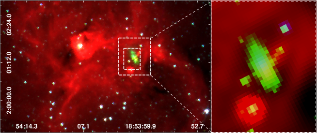
Figure 1: Left: Spitzer-IRAC three color image (3.6 $\mu$m $=$ blue, 4.5 $\mu$m $=$ green and 8 $\mu$m $=$ red). The dashed rectangles are the regions mapped in ¹²CO J=3–2 and HCO⁺ J=4–3 (the largest one) and in ¹³CO J=3–2 and CS J=7–6 (the smallest one). Right: zoom in of the surveyed region.

Cyganowski et al. (2008) identified more than 300 Galactic extended 4.5 $\mu$m sources, naming extended green objects (EGOs) or “green fuzzies”, for the common coding of the [4.5 $\mu$m] band as green in three-color composite Infrared Array Camera images from the Spitzer Telescope. According to the authors, an EGO is a probable massive young stellar object (MYSO) driving outflows. The extended emission in the 4.5 $\mu$m band is supposed to be due to H₂ ($\nu=0-0$, S(9,10,11)) lines and CO ($\nu=1-0$) band heads, that are excited by the shock of the outflows propagating in the interstellar medium (see Noriega-Crespo et al. 2004; Marston et al. 2004; Smith & Rosen 2005). Recently, De Buizer & Vacca (2010) reported the first direct spectroscopic identification of the origin of the 4.5 $\mu$m emission towards two EGOs using NIRI on the Gemini North telescope. In one of the observed EGOs, they proved that the 4.5 $\mu$m emission is due primarily to lines of molecular hydrogen, which are collisionally excited.

EGO G35.03+0.35 (hereafter EGOg35) is embedded in a dense molecular cloud at the distance of 3.5 kpc (Petriella et al., 2010) located on the border of the infrared dust bubble N65 (Churchwell et al., 2006, 2007). According to Petriella et al. (2010) there are several young stellar object (YSO) candidates around N65, being EGOg35 the most prominent source. Using IR and sub-mm fluxes measured from this EGO, the authors performed an spectral energy distribution (SED), showing that this source is indeed a massive stellar object at the earlier stages of evolution with outflowing activity. The 4.5 $\mu$m emission of this EGO has a bipolar morphology, with one lobe to the NE and the other to the SW. The source presents maser emission of several molecular lines (see e.g. Forster & Caswell 1989; Caswell et al. 1995; Kurtz & Hofner 2005). Recently, CH₃OH maser emission at 6.7 and 44 GHz has been detected and analysed by Cyganowski et al. (2009). The 6.7 GHz CH₃OH masers are radiatively pumped by IR emission from the warm dust associated exclusively with massive YSOs, while the methanol maser at 44 GHz is collisionally excited in molecular outflows, and particularly at interfaces between outflows and the surrounding ambient cloud (see Cyganowski et al. 2009 and references therein).

Considering that EGOg35 is indeed a massive YSO evolving in a dense molecular medium, it is important to understand the physical characteristics of its ambient medium. We investigated this ambient through several molecular lines obtained with the Atacama Submillimeter Telescope Experiment (ASTE). The results of this investigation are presented in this work.

2 Observations

The molecular observations were performed on July 14 and 15, 2010 with the 10 m Atacama Submillimeter Telescope Experiment (ASTE; Ezawa et al. 2004). We used the CATS345 GHz band receiver, which is a two-single band SIS receiver remotely tunable in the LO frequency range of 324-372 GHz. We simultaneously observed ¹²CO J=3–2 at 345.796 GHz and HCO⁺ J=4–3 at 356.734 GHz, mapping a region of 70^′′ $\times$ 80^′′ centered at RA $=$ 18^h54^m0.7^s, dec. $=+$02^∘01^′18.9^′′, J2000). We also observed ¹³CO J=3–2 at 330.588 GHz and CS J=7–6 at 342.883 GHz towards the same center mapping a region of 40^′′ $\times$ 50^′′. The mapping grid spacing was 10^′′ and the integration time was 60 sec per pointing in both cases. All the observations were performed in position switching mode. We verified that the off position (RA $=$ 18^h53^m55.8^s, dec. $=+$02^∘07^′49.5^′′, J2000) was to be free of emission.

We used the XF digital spectrometer with a bandwidth and spectral resolution set to 128 MHz and 125 kHz, respectively. The velocity resolution was 0.11 km s^-1 and the half-power beamwidth (HPBW) was 22^′′, for all observed molecular lines. The system temperature varied from T${}_{\rm sys}=150$ to 200 K. The main beam efficiency was $\eta_{\rm mb}\sim 0.65$. The spectra were Hanning smoothed to improve the signal-to-noise ratio and only linear or/and some third order polynomia were used for baseline fitting. The data were reduced with NEWSTAR and the spectra processed using the XSpec software package.

To complement the molecular data we use near- and mid-IR and radio continuum data from public databases and catalogues, which are described in the corresponding sections.

3 Results and discussion

The source EGO G35.03$+$0.35 (EGOg35) is located at the border of an HII region which is delineated mainly by the 8 $\mu$m emission. Figure 1 (left) shows a composite three-color image of a region towards EGOg35. The image displays three Spitzer-IRAC bands: 3.6 $\mu$m (in blue), 4.5 $\mu$m (in green) and 8 $\mu$m (in red). EGOg35 is the green structure inside the dashed rectangles, which represent the 70^′′ $\times$ 80^′′ and 40^′′ $\times$ 50^′′ regions mapped in the molecular lines as described in the previous section. A zoom in of the surveyed region is shown in Fig. 1 (right).

3.1 Molecular lines

To study the molecular ambient where EGOg35 is embedded, we analyse the ¹²CO and ¹³CO J=3–2, HCO⁺ J=4–3 and CS J=7–6 transitions, tracers of outflows and dense gas. Figures 2 and 3 display the molecular lines spectra obtained towards EGOg35. Most of the spectra are far of having a simple Gaussian shape, presenting asymmetries, probable absorption dips, and spectral wings or shoulders, which suggest that the molecular gas is affected by the dynamics of EGOg35. In what follows we study the gas kinematics.

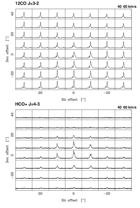
Figure 2: ¹²CO J=3–2 and HCO⁺ J=4–3 spectra obtained towards EGOg35.

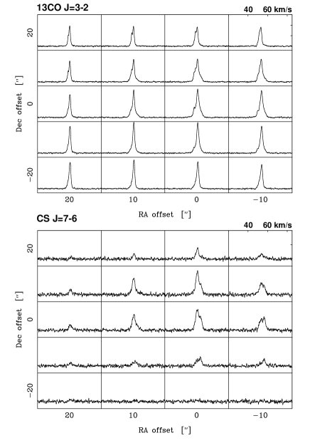
Figure 3: ¹³CO J=3–2 and CS J=7–6 spectra obtained towards EGOg35.

Figure 4: Spectra towards the center of the observed region. The HCO⁺ J=4–3 and CS J=7–6 lines were scaled with a factor of $\times 3$. The vertical axis is main beam brightness temperature.

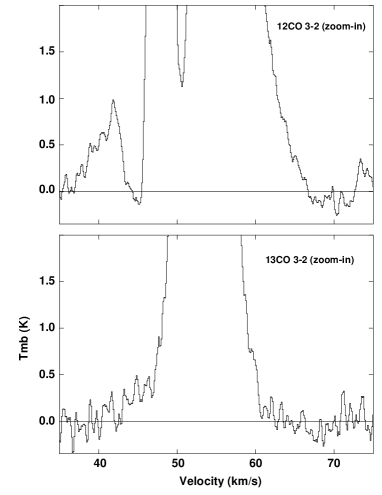
Figure 5: Zoom-in of the ¹²CO and ¹³CO J=3–2 profiles presented in Fig. 4 in the intensity range going from $-0.35$ to 2 K.

Figure 4 shows the spectra obtained towards the central position of EGOg35, that is the (0,0) offset in Figs. 2 and 3. In the case of the HCO⁺ J=4–3 and CS J=7–6 lines, their brightness temperatures were scaled with a factor of $\times 3$. Figure 5 displays a zoom-in of the central ¹²CO and ¹³CO J=3–2 profiles in the intensity range that goes from $-0.35$ to 2 K, in order to note some weak features. In the case of the ¹²CO line can be appreciated a weak component ($\sim 5$ times above the rms noise) centered at $\sim 41$ km s^-1. The parameters determined from Gaussian fitting of these lines are presented in Table 1. T_mb represents the peak brightness temperature, V_LSR the central velocity referred to the Local Standard of Rest. Errors are formal 1$\sigma$ value for the model of the Gaussian line shape. All the lines were well fit with more than one Gaussian function, which very likely indicates the presence of several components or/and spectral wings, usually signatures of outflows. In Table 2 we present V_max and V_min, indicating the respective total widths of the spectra considering all the components, and $\int{T_{mb}dv}$, the intensity integrated over the whole profile.

The ¹²CO J=3–2 spectrum presented in Fig. 4 shows a double peak structure like with a main component centered at $\sim$54.2 km s^-1 and a less intense component centered at $\sim$48.7 km s^-1. The ¹³CO J=3–2 spectrum presents similar features. We conclude that these lines present an absorption dip at $\sim$51.5 km s^-1 which separates both mentioned velocity components, showing that the lines are self-absorbed as it is usually found towards star-forming regions (Johnstone et al., 2003; Buckle et al., 2010; Ortega et al., 2010). The velocity of the mentioned ¹²CO and ¹³CO dip is coincident (within the errors) with the central velocities of the SiO (5–4), H¹³CO⁺ (3–2), and CH₃OH (5_2,3–4_1,3) lines observed towards the center of EGOg35 by Cyganowski et al. (2009) and with the CS J=7–6 main component reported in this work. Therefore, we conclude that v $\sim$51.5 km s^-1 is the velocity of the ambient gas, and the other reported components (see Table 1) may be related to outflows or/and high velocity material. In Section 3.2 we analyse this contention.

Table 1: Observed parameters of the molecular lines shown in Figure 4.

Emission	Tmb	VLSR
	(K)	(km s-1)
12CO J=3–2	0.80 $\pm$0.20	41.12 $\pm$0.56
	4.55 $\pm$0.25	48.68 $\pm$1.25
	12.40 $\pm$0.75	54.20 $\pm$1.20
	4.42 $\pm$1.50	56.90 $\pm$1.20
	3.65 $\pm$0.85	59.10 $\pm$1.25
13CO J=3–2	4.40 $\pm$0.45	50.10 $\pm$1.60
	12.85 $\pm$1.70	53.50 $\pm$1.40
	2.48 $\pm$0.60	56.75 $\pm$1.50
HCO+ J=4–3	3.10 $\pm$0.8	52.55 $\pm$0.75
	2.60 $\pm$0.8	56.05 $\pm$0.85
CS J=7–6	2.85 $\pm$0.35	53.15 $\pm$0.65
	1.45 $\pm$0.60	57.05 $\pm$0.50

Table 2: Derived parameters of the molecular lines shown in Figure 4.

Emission	Vmin	Vmax	$\int{T_{mb}dv}$
	(km s-1)	(km s-1)	(K km s-1)
12CO J=3–2	37.0	67.0	92.4 $\pm$1.9
13CO J=3–2	44.5	60.2	64.2 $\pm$1.8
HCO+ J=4–3	45.5	61.6	15.5 $\pm$0.7
CS J=7–6	47.7	60.7	16.6 $\pm$0.8

Regarding the HCO⁺ J=4–3 emission, the profiles towards the center of the surveyed region present a dip at v $\sim 54$ km s^-1 (see Fig. 2 bottom, and Fig. 4). Cyganowski et al. (2009) presented a single point observation of H¹³CO⁺ J=4–3 towards EGOg35. They report that the H¹³CO⁺ J=4–3 emission peaks at $\sim 53.1$ km s^-1 with a FWHM $\Delta$v $\sim 5.4$ km s^-1. Taking into account that the H¹³CO⁺ emission is optical thinner than the HCO⁺ emission and peaks at a velocity close to that of the HCO⁺ dip, we conclude that this emission indeed appears self-absorbed. This kind of spectral feature might be revealing the existence of a density gradient in the clump (Hiramatsu et al., 2007), consistent with the presence of an embedded central source with outflowing activity. It is known that such molecular species enhances in molecular outflows (Rawlings et al., 2004). In effect, a strong enhancement of the HCO⁺ abundance is expected to occur in the boundary layer between the outflow jet and the surrounding molecular core. This would be due to the liberation and photoprocessing by the shock of the molecular material stored in the icy mantles of the dust. Figure 6 displays the HCO⁺ J=4–3 emission integrated between 45 and 62 km s^-1, showing a HCO⁺ molecular clump peaking at the position of EGOg35.

Figure 6: HCO⁺ J=4–3 emission integrated between 45 and 62 km s^-1. The beam size is 22^′′.

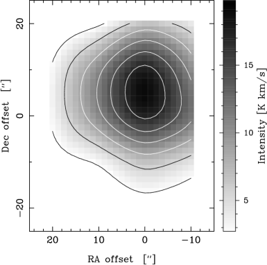
Figure 7: CS J=7–6 emission integrated between 45 and 62 km s^-1. The beam size is 22^′′.

It is worth noting that the central HCO⁺ and CS spectra, which survey the densest region where EGOg35 is embedded, have the closer component (i.e. the component with lower velocity, or blue component) stronger than the farthest one (red component). This signature suggests the presence of infalling gas, which is consistent with the presence of a YSO accreting material. As Zhou et al. (1993) explain, this effect reflects the fact that the excitation of molecules is higher in the cloud center and, if the cloud has infalling motion, then the observer is looking at the hotter side of the blue hemisphere and the cooler side of the red hemisphere. Therefore, the blue emission should always be as strong as, or stronger than, the red emission.

Finally, it is important to note that the CS J=7–6 emission maps the dense envelope where the massive YSO is evolving. The detection of this line implies the presence of a gaseous envelope with temperatures and densities above 40 K and $6\times 10^{6}$ cm^-3, respectively (e.g. Takakuwa et al. 2007). Figure 7 shows the CS J=7–6 emission integrated between 45 and 62 km s^-1.

3.1.1 Column densities and abundances

To estimate the molecular column densities and hence the abundances in the region we assume as a first order approximation local thermodynamic equilibrium (LTE) and a beam filling factor of 1. From the peak temperature ratio between the CO isotopes (¹²T_mb/¹³T_mb; taken from the CO main components at v $\sim 54$ km s^-1), it is possible to estimate the optical depths from (e.g. Scoville et al. 1986):

$$\frac{{}^{12}{\rm T}_{mb}}{{}^{13}{\rm T}_{mb}}=\frac{1-exp(-\tau_{12})}{1-exp(-\tau_{12}/X)}$$ (1)

where $\tau_{12}$ is the optical depth of the ¹²CO gas and $X=$ [¹²CO]/[¹³CO] is the isotope abundance ratio. Assuming R${}_{\odot}=8$ and using [¹²CO]/[¹³CO] $=(6.21\pm 1.00){\rm D_{GC}}+(18.71\pm 7.37)$ (Milam et al., 2005) where D${}_{\rm GC}=5.5$ kpc is the distance between the source and the Galactic Center, we obtain [¹²CO]/[¹³CO] $=53\pm 12$. Then the ¹²CO J=3–2 optical depth is $\tau_{12}\sim 300$, while the ¹³CO J=3–2 optical depth is $\tau_{13}\sim 6$, revealing that both lines are optically thick. Thus, we calculate the excitation temperature from

$$T_{ex}(3\rightarrow 2)=\frac{16.95{\rm K}}{{\rm ln}[1+16.59{\rm K}/(T_{\rm max}(^{12}{\rm CO})+0.036{\rm K})]}$$ (2)

obtaining $T_{ex}\sim 20$ K. Then, we derive de ¹³CO and ¹²CO column densities from (see e.g. Buckle et al. 2010):

$${\rm N(^{13}CO)}=8.28\times 10^{13}~{}e^{\frac{15.87}{T_{ex}}}\frac{T_{ex}+0.88}{1-exp(\frac{-15.87}{T_{ex}})}\int{\tau_{13}{\rm dv}}$$ (3)

and

$${\rm N(^{12}CO)}=7.96\times 10^{13}~{}e^{\frac{16.6}{T_{ex}}}\frac{T_{ex}+0.92}{1-exp(\frac{-16.6}{T_{ex}})}\int{\tau_{12}{\rm dv}}$$ (4)

where, taking into account that $\tau\geq 1$ in both cases, we use the approximation:

$$\int{\tau~{}{\rm dv}}=\frac{1}{J(T_{ex})-J(T_{\rm BG})}\frac{\tau}{1-e^{-\tau}}\int{{\rm T_{mb}~{}dv}}$$ (5)

with

$$J(T)=\frac{h\nu/k}{exp(\frac{h\nu}{kT})-1}$$ (6)

We obtain N(¹³CO) $\sim 7\times 10^{16}$ cm^-2 and N(¹²CO) $\sim 1\times 10^{19}$ cm^-2.

Additionally, we derive the CS J=7–6 and HCO⁺ J=4–3 column densities from:

$${\rm N(CS)}=2.54\times 10^{11}~{}e^{\frac{49.4}{T_{ex}}}\frac{T_{ex}+0.56}{1-exp(\frac{-16.45}{T_{ex}})}\int{\tau{\rm dv}}$$ (7)

and

$${\rm N(HCO^{+})}=5.85\times 10^{10}~{}e^{\frac{25.7}{T_{ex}}}\frac{T_{ex}+0.71}{1-exp(\frac{-17.12}{T_{ex}})}\int{\tau{\rm dv}}$$ (8)

Since the CS J=7–6 line is optically thick (e.g. Giannini et al. 2005), we use again the approximation presented in equation (5) assuming $\tau_{\rm CS}=1$. On the other hand, by assuming that the HCO⁺ J=4–3 is optically thin, we use the approximation:

$$\int{\tau~{}{\rm dv}}=\frac{1}{J(T_{ex})-J(T_{\rm BG})}\int{{\rm T_{mb}~{}dv}}$$ (9)

We adopt as excitation temperatures 66 K and 43 K for the CS and HCO⁺, respectively, which correspond to the equivalent temperature of each molecular transition. We therefore obtain N(CS) $\sim 8\times 10^{13}$ cm^-2 and N(HCO⁺) $\sim 9.5\times 10^{12}$ cm^-2.

Assuming the abundance ratio [H₂]/[¹³CO] $=77\times 10^{4}$ (Wilson & Rood, 1994), from the N(¹³CO) we can estimate the H₂ column density in N(H₂) $\sim 5\times 10^{22}$ cm^-2. This value is in agreement with the H₂ column densities reported for high-mass protostar candidates associated with methanol masers (Codella et al., 2004; Szymczak et al., 2007), as in our case. Thus, using this H₂ column density we derive the abundance ratios for the HCO⁺ and CS: X(HCO⁺) $\sim 2\times 10^{-10}$ and X(CS) $\sim 1.6\times 10^{-9}$. The X(CS) value is within the very wide range ($5\times 10^{-10}-2\times 10^{-7}$) measured in the outflows of protostars (e.g. Bottinelli & Williams 2004; Jørgensen et al. 2004; Giannini et al. 2005).

3.1.2 High velocity material and outflows

As discussed in Section 3.1, the ¹²CO J=3–2 spectrum obtained towards the center of EGOg35 shows several components, some of them suggesting outflowing activity from EGOg35. The presence of outflows or high velocity material moving along the line of sight can be proven by comparing the ¹²CO emission with the higher density tracer CS J=7–6. Figure 8 presents the ¹²CO and CS spectra towards the center of the region with vertical lines remarking the ranges where ¹²CO emission is detected at higher and lower velocities with respect to the CS. This figure confirms the presence of ¹²CO spectral wings, which should be due to a red outflow going from 59.6 to 66.5 km s^-1 and a blue one, extending from 37.0 to 48.9 km s^-1. In the case of the blue wing, we consider that the weak ¹²CO component centered at $\sim$41 km s^-1 is part of the source outflows because its velocity is compatible with that of the 6.7 GHz methanol maser detected by Cyganowski et al. (2009), confirming that this ¹²CO component is due to the gas expansion caused by EGOg35.

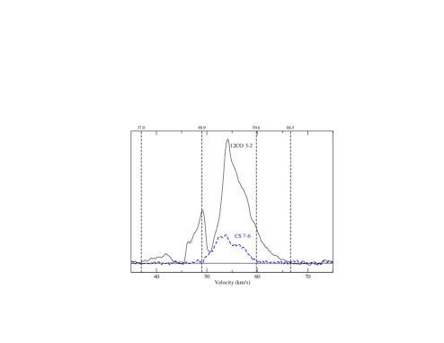
Figure 8: ¹²CO J=3–2 (solid line) and CS J=7–6 (dashed line) towards the center of EGOg35. The vertical lines remark the ranges where ¹²CO emission is detected at higher and lower velocities with respect to the CS.

To analyze the velocity and spatial distribution of the ¹²CO J=3–2 emission, in Fig. 9 we present integrated velocity channel maps every $\sim$1.1 km s^-1. The spatial distributions of the blue and red wings are shown in channels going from $\sim 36$ km s^-1 to 50 km s^-1 , and $\sim 57$ km s^-1 to 64 km s^-1, respectively. Figure 10 displays the 4.5 $\mu$m emission with contours of the ¹²CO J=3–2 line integrated from 37 to 49 km s^-1 and 58 to 66 km s^-1 (blue thick and red thin contours, respectively).

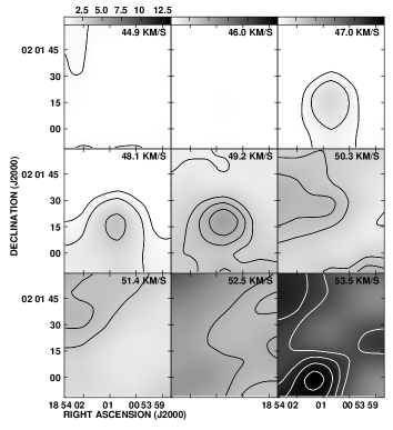
Figure 9: Integrated velocity channel maps of the ¹²CO J=3–2 emission every $\sim$ 1.1 km s^-1. The grayscale is displayed at the top of each figure and is in K km s^-1, the contour levels are 0.05, 0.2, 0.4, and 0.7 K km s^-1 for the first panel, 0.5, 1, 3, 4, 4.5, 10, 11, 12.5 K km s^-1 for the second panel, and 0.5, 1, 2.5, 5, 7.5, 10, 12.5, 15 K km s^-1, for the third one. The beam size is 22^′′.

Figure 10: In grays is displayed the 4.5 $\mu$m emission from EGOg35. The blue thick and the red thin contours show the ¹²CO J=3–2 emission integrated from 37 to 49 km s^-1 and 58 to 66 km s^-1, respectively. The levels are 6.5, 9.5, and 12.5 K km s^-1 for the blue emission and 4, 10, and 16 K km s^-1 for the red one. The dashed square is the surveyed area.

In what follows, from the ¹²CO spectral wings we estimate the mass and energy to study the dynamics involved in the EGOg35 outflowing activity. Using $M=\mu m_{H}d^{2}\Omega X({\rm CO})^{-1}{\rm N(CO)}$, we obtain the mass for the red and blue molecular outflows. N(CO) is the ¹²CO column density, $d$ the distance, $m_{H}$ the hydrogen atom mass, we adopt a mean molecular weight per H₂ molecule of $\mu=2.72$ to include helium, $\Omega$ is the area of the ¹²CO red and blue clumps shown in Figs. 9 and 10, and $X({\rm CO})=10^{-4}$ is the ¹²CO relative abundance (Frerking et al., 1982). Integrating the ¹²CO emission from 58 to 66 km s^-1 we obtain a N(CO)${}_{red}\sim 2.1\times 10^{17}$ cm^-2 and $M_{red}\sim 5$ M_⊙, while integrating from 37 to 49 km s^-1 we obtain N(CO)_blue $\sim 1.1\times 10^{18}$ cm^-2 and $M_{blue}\sim 24$ M_⊙. We calculate the momentum and energy of the red and blue components using:

$$P=MV$$ (10)

$$E_{k}=\frac{1}{2}MV^{2}$$ (11)

where $V$ is a characteristic velocity estimated as the difference between the maximum velocity of detectable ¹²CO emission in the red and blue wings respectively, and the molecular ambient velocity ($\sim 51.5$ km s^-1), being $V_{red}\sim 14.5$ km s^-1 and $V_{blue}\sim 14.5$ km s^-1. Thus, we obtain $P_{red}=72$ M_⊙km s^-1 and $E_{k}^{red}=510$ M_⊙[km s^-1]² ($E_{k}^{red}\sim 1\times 10^{46}$ ergs), and $P_{blue}=350$ M_⊙km s^-1 and $E_{k}^{blue}=2500$ M_⊙[km s^-1]² ($E_{k}^{blue}\sim 5\times 10^{46}$ ergs). The obtained outflows parameters are summarized in Table 3.

Table 3: Outflow parameters.

Shift	N(CO)	M	$P$	$E_{k}$
	($\times 10^{18}$ cm-2)	(M⊙)	(M⊙km s-1)	(M⊙[km s-1]2)
Red	0.21	5	72	510
Blue	1.10	24	350	2500

The derived mass and energy for the outflows discovered towards EGOg35 are similar to those of massive and energetic molecular outflows driven by high-mass YSOs (Beuther et al., 2002; Wu et al., 2004). We do not provide estimates of outflow dynamical timescale and mass rate because the analysed high velocity material is aligned along the line of sight, and therefore it is not possible to estimate the lengths of the outflow lobes. In fact, with the moderate angular resolution of the present observations, it is possible that we miss the emission of the outflows along the plane of the sky. Molecular observations with higher angular resolution are needed to spatially resolve the outflows.

3.2 Spectral energy distribution

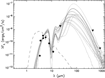
Figure 11: Spectral energy distributions of the EGO G35.03+0.35. The black line correspond to the best fitting model and the gray lines to the following 19 best models. The dashed line is the photosphere model of the central source in the best fitting model.

Petriella et al. (2010) performed a spectral energy distribution (SED) of EGOg35 concluding that the source is indeed a massive YSO. Taking into account that at present it is available new mid-IR fluxes obtained from WISE Preliminary Release Source Catalog, in this section we perform a new SED of the source to study with more accuracy its physical parameters. The advantage of this new SED is that the WISE data present fluxes at 3.4, 4.6, 12, and 22 $\mu$m bands, being of importance the last two bands, mainly the 12 $\mu$m, because the SED of a YSO usually presents the separation between the contributions from the disk and envelope fluxes around this wavelength. Thus, we fit the SED using the tool developed by Robitaille et al. (2007). We use the fluxes in the four Spitzer-IRAC bands obtained from Cyganowski et al. (2008) together with the WISE fluxes, and the SCUBA bands at 450 and 850 $\mu$m (source G35.02+0.35, Hill et al. 2006). The fluxes at 22 $\mu$m from WISE and SCUBA bands were taken as upper limits as they have lower angular resolution and they can include contributions from other sources around EGOg35. As done in Petriella et al. (2010) we assume an interstellar absorption between 15 and 35 magnitudes and a distance range between 3 and 4 kpc. In Fig. 11 we show the SEDs of the 20 best fitting models. The solid black line represents the best fitting model from which we obtain the following parameters: $M_{\star}\sim 23$ M_⊙, $M_{env}\sim 1280$ M_⊙, and $\dot{M}_{env}\sim 0.03$ M${}_{\odot}/yr$. We do not report the disk mass because is not well constrained in the SED fitting. As Robitaille et al. (2007) point out, in the early stages of evolution, when the disk is deeply embedded inside the infalling envelope, the relative contributions of the disk and envelope to the SED are difficult to disentangle.

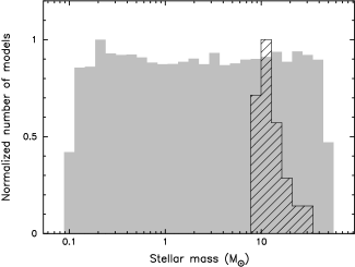
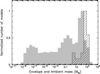
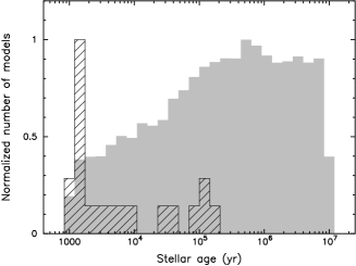
Figure 12: Distribution of some physical parameters (central source mass, envelope mass, and age) of the 20 best fitting models (hashed columns) together with the distribution of all the models (gray columns).

Following the Robitaille et al. (2006) evolutionary classification, the best fitting model (and also the following 80 fitting models) correspond to a stage I YSO, i.e., a protostar with large accretion envelope. In Fig. 12 we present the histograms with the distribution of the constrained physical parameters. The hashed columns represent the 20 best fitting models and the gray columns correspond to all the models of the grid. We remark that the 20 best fitting models correspond to massive central sources (between 8 and 20 M_⊙) surrounded by massive envelopes with large accretion rates. Regarding the age of the source, there is a high dispersion in the results (ages range from $10^{3}$ to $10^{5}$ years) but the presence of a massive envelope is a strong evidence that the source is at the earliest evolutionary stage.

3.3 Radio continuum analysis

Figure 13: Radio continuum emission at 8.4 GHz displayed in contours of 0.3, 1, and 10 mJy beam^-1 over the IRAC-Spitzer 4.5 $\mu$m emission. The radio continuum has a beam of 1$\aas@@fstack{\prime\prime}$4 $\times$ 1$\aas@@fstack{\prime\prime}$0 while the angular resolution of the mid-IR emission is about 1$\aas@@fstack{\prime\prime}$5.

We investigate the radio continuum emission at 8.4 GHz of EGOg35. To produce the image we used archival data from observations performed with the VLA telescope operating in its B configuration on May 7 and 14, 2009 (project code AC948). Data processing was carried out using MIRIAD software package. The final image has an angular resolution of 1$\aas@@fstack{\prime\prime}$4 $\times$ 1$\aas@@fstack{\prime\prime}$0 and an rms noise of 0.1 mJy beam^-1. Figure 13 shows, in contours, the radio continuum emission of EGOg35 over its mid-IR emission at 4.5 $\mu$m. As can be seen from this figure, there are three radio sources: source A which coincides with the IR southwestern lobe of the EGOg35, source B that appears in between the IR lobes, and source C, marginally detected, which is projected onto the northeastern lobe of the EGO. The radio source A, the brightest and the only one resolved with this data set, is centered at 18^h54^m00.49^s, $+$02^∘01^′18.20^′′ (J2000), and has an integrated flux density of 13.5 mJy. The source B is centered at 18^h54^m00.66^s, $+$02^∘01^′19.40^′′ (J2000) and has a peak intensity of 1 mJy beam^-1, and source C is centered at 18^h54^m00.76^s, $+$02^∘01^′22.62^′′ (J2000) and its peak has a flux density of 0.3 mJy beam^-1. Source A and B were also detected at 44 GHz with a similar angular resolution by Cyganowski et al. (2009). The authors reported an integrated flux density of 12.7 mJy for the brightest radio source and a peak flux density of 3.6 mJy beam^-1 for source B. We calculate the spectral index $\alpha$ (S $\propto\nu^{\alpha}$) between both frequencies, being $\alpha\sim-0.05$ for source A, and $\alpha\sim+0.77$ for source B. The radio spectral index of the radio source A is consistent with emission from an UCHII region, while the value obtained for source B suggests that its radio emission could be due either to an HCHII region (Kurtz, 2005) or to a constant-velocity ionized wind source (Panagia & Felli, 1975).

From this radio continuum analysis we can suggest the presence of several young stellar objects in the region. The fact that these radio sources overlap the 4.5 $\mu$m emission reinforces the hypothesis that the infrared emission originates in YSO shocks.

4 Summary

The extended green object EGO G35.03$+$0.35 (EGOg35, in this work), a massive YSO, is embedded in a molecular clump located at the border of an HII region. In this work we investigated the surrounding molecular gas through several molecular species using the Atacama Submillimeter Telescope Experiment (ASTE). We observed and analysed the ¹²CO and ¹³CO J=3–2, HCO⁺ J=4–3 and CS J=7–6 transitions, which are useful to trace outflows and dense gas. To complement our analysis we used IR and radio continuum data from public database. In what follows we summarize the main results of our work:

(1) Most of the molecular spectra observed towards the surveyed region are far of having a simple Gaussian shape, presenting asymmetries, absorption dips, and spectral wings or shoulders, characteristics that strongly suggest the existence of kinematical perturbations in the gas originated in the object EGOg35.

(2) The ¹²CO J=3–2 line towards EGOg35 shows a double peak structure like with a main component centered at $\sim$54 km s^-1, a less intense component centered at $\sim$48 km s^-1, and an absorption dip at $\sim$51.5 km s^-1. The line also presents spectral wings due to the ouflowing activity of EGOg35. We obtained a total mass and kinetic energy for the YSO outflows of 30 M_⊙ and 3000 M_⊙[km s^-1]² ($6\times 10^{46}$ ergs), respectively, similar to those found towards other massive and energetic molecular outflows driven by high-mass YSOs.

(3) We discovered a HCO⁺ clump towards EGOg35, supporting the presence of outflows in the region because it is known that such molecular species enhances in the boundary layer between the outflow jet and the surrounding molecular core. The central HCO⁺ spectra present an absorption dip at v $\sim 54$ km s^-1 due to self-absorbed gas, which is probably revealing the existence of a density gradient in the clump.

(4) We discovered a CS clump towards EGOg35. The CS J=7–6 emission maps the dense envelope where the massive YSO is evolving, and its detection implies the presence of molecular gas with temperatures and densities above 40 K and $6\times 10^{6}$ cm^-3, respectively.

(5) The central HCO⁺ and CS spectra, which survey the densest region where EGOg35 is embedded, show two velocity components with the closer one (blue component) stronger than the farthest one (red component). This signature suggests that these lines are mapping infalling gas, which is consistent with the presence of a YSO accreting material.

(6) From the spectral energy distribution (SED) study we confirm that EGOg35 is a massive YSO at the earliest evolutionary stage (i.e. a class I YSO).

(7) Analysing radio continuum emission towards EGOg35 we conclude that there is evidence of the presence of an UCHII region and another source that could be either an HCHII region or a constant-velocity ionized wind source. The radio continuum analysis suggests the presence of several possible young stellar objects in the region. Future multiwavelength observations with very high angular resolution will be of a great importance to go deeper in the study of this region.

References

- Beuther et al. (2002) Beuther H., Schilke P., Sridharan T. K., Menten K. M., Walmsley C. M., Wyrowski F., 2002, A&A, 383, 892
- Bottinelli & Williams (2004) Bottinelli S., Williams J. P., 2004, A&A, 421, 1113
- Buckle et al. (2010) Buckle J. V., Curtis E. I., Roberts J. F., et al., 2010, MNRAS, 401, 204
- Caswell et al. (1995) Caswell J. L., Vaile R. A., Ellingsen S. P., Whiteoak J. B., Norris R. P., 1995, MNRAS, 272, 96
- Churchwell et al. (2006) Churchwell E., Povich M. S., Allen D., et al., 2006, ApJ, 649, 759
- Churchwell et al. (2007) Churchwell E., Watson D. F., Povich M. S., et al., 2007, ApJ, 670, 428
- Codella et al. (2004) Codella C., Lorenzani A., Gallego A. T., Cesaroni R., Moscadelli L., 2004, A&A, 417, 615
- Curtis et al. (2010) Curtis E. I., Richer J. S., Swift J. J., Williams J. P., 2010, MNRAS, 408, 1516
- Cyganowski et al. (2009) Cyganowski C. J., Brogan C. L., Hunter T. R., Churchwell E., 2009, ApJ, 702, 1615
- Cyganowski et al. (2008) Cyganowski C. J., Whitney B. A., Holden E., et al., 2008, AJ, 136, 2391
- De Buizer & Vacca (2010) De Buizer J. M., Vacca W. D., 2010, AJ, 140, 196
- Ezawa et al. (2004) Ezawa H., Kawabe R., Kohno K., Yamamoto S., 2004, in Society of Photo-Optical Instrumentation Engineers (SPIE) Conference, Vol. 5489, Society of Photo-Optical Instrumentation Engineers (SPIE) Conference Series, Oschmann Jr. J. M., ed., pp. 763–772
- Forster & Caswell (1989) Forster J. R., Caswell J. L., 1989, A&A, 213, 339
- Frerking et al. (1982) Frerking M. A., Langer W. D., Wilson R. W., 1982, ApJ, 262, 590
- Giannini et al. (2005) Giannini T., Massi F., Podio L., Lorenzetti D., Nisini B., Caratti o Garatti A., Liseau R., Lo Curto G., Vitali F., 2005, A&A, 433, 941
- Hill et al. (2006) Hill T., Thompson M. A., Burton M. G., Walsh A. J., Minier V., Cunningham M. R., Pierce-Price D., 2006, MNRAS, 368, 1223
- Hiramatsu et al. (2007) Hiramatsu M., Hayakawa T., Tatematsu K., Kamegai K., Onishi T., Mizuno A., Yamaguchi N., Hasegawa T., 2007, ApJ, 664, 964
- Johnstone et al. (2003) Johnstone D., Boonman A. M. S., van Dishoeck E. F., 2003, A&A, 412, 157
- Jørgensen et al. (2004) Jørgensen J. K., Hogerheijde M. R., Blake G. A., van Dishoeck E. F., Mundy L. G., Schöier F. L., 2004, A&A, 415, 1021
- Kurtz (2005) Kurtz S., 2005, in IAU Symposium, Vol. 227, Massive Star Birth: A Crossroads of Astrophysics, R. Cesaroni, M. Felli, E. Churchwell, & M. Walmsley, ed., pp. 111–119
- Kurtz & Hofner (2005) Kurtz S., Hofner P., 2005, AJ, 130, 711
- Marston et al. (2004) Marston A. P., Reach W. T., Noriega-Crespo A., et al., 2004, ApJS, 154, 333
- Milam et al. (2005) Milam S. N., Savage C., Brewster M. A., Ziurys L. M., Wyckoff S., 2005, ApJ, 634, 1126
- Noriega-Crespo et al. (2004) Noriega-Crespo A., Morris P., Marleau F. R., et al., 2004, ApJS, 154, 352
- Ortega et al. (2010) Ortega M. E., Paron S., Cichowolski S., Rubio M., Castelletti G., Dubner G., 2010, A&A, 510, A96+
- Panagia & Felli (1975) Panagia N., Felli M., 1975, A&A, 39, 1
- Petriella et al. (2010) Petriella A., Paron S., Giacani E., 2010, A&A, 513, A44
- Rawlings et al. (2004) Rawlings J. M. C., Redman M. P., Keto E., Williams D. A., 2004, MNRAS, 351, 1054
- Robitaille et al. (2007) Robitaille T. P., Whitney B. A., Indebetouw R., Wood K., 2007, ApJS, 169, 328
- Robitaille et al. (2006) Robitaille T. P., Whitney B. A., Indebetouw R., Wood K., Denzmore P., 2006, ApJS, 167, 256
- Scoville et al. (1986) Scoville N. Z., Sargent A. I., Sanders D. B., Claussen M. J., Masson C. R., Lo K. Y., Phillips T. G., 1986, ApJ, 303, 416
- Smith & Rosen (2005) Smith M. D., Rosen A., 2005, MNRAS, 357, 1370
- Szymczak et al. (2007) Szymczak M., Bartkiewicz A., Richards A. M. S., 2007, A&A, 468, 617
- Takakuwa et al. (2007) Takakuwa S., Kamazaki T., Saito M., Yamaguchi N., Kohno K., 2007, PASJ, 59, 1
- Wilson & Rood (1994) Wilson T. L., Rood R., 1994, ARA&A, 32, 191
- Wu et al. (2004) Wu Y., Wei Y., Zhao M., Shi Y., Yu W., Qin S., Huang M., 2004, A&A, 426, 503
- Zhou et al. (1993) Zhou S., Evans II N. J., Koempe C., Walmsley C. M., 1993, ApJ, 404, 232