Bayesian angular power spectrum analysis of interferometric data

Abstract

We present a Bayesian angular power spectrum and signal map inference engine which can be adapted to interferometric observations of anisotropies in the cosmic microwave background, 21 cm emission line mapping of galactic brightness fluctuations, or 21 cm absorption line mapping of neutral hydrogen in the dark ages. The method uses Gibbs sampling to generate a sampled representation of the angular power spectrum posterior and the posterior of signal maps given a set of measured visibilities in the $uv$-plane. We use a mock interferometric CMB observation to demonstrate the validity of this method in the flat-sky approximation when adapted to take into account arbitrary coverage of the $uv$-plane, mode-mode correlations due to observations on a finite patch, and heteroschedastic visibility errors. The computational requirements scale as $\mathcal{O}(n_{p}\log n_{p})$ where $n_{p}$ measures the ratio of the size of the detector array to the inter-detector spacing, meaning that Gibbs sampling is a promising technique for meeting the data analysis requirements of future cosmology missions.

1. Introduction

Interferometric techniques have several advantages compared to single-dish observations: for high resolution experiments they perform the same work of an optical system but with large potential weight and size reductions, they are naturally differential and hence well-adapted to measurements of small anisotropies superimposed on a large isotropic background, their noise characteristics are highly uncorrelated to a good approximation, and they are well-suited for observations of statistically isotropic anisotropies, in which the signal correlations naturally decouple in Fourier space (Thompson et al. 2001). Additionally, a revolution in the development of efficient digital correlator technology, leading to massive reductions in power requirements (Parsons et al. 2008), has brought interferometric approaches back to the list of contenders for strategies for a future space-based cosmic microwave background (CMB) mission (Timbie & Tucker 2009).

Already, interferometers have made great strides in measuring CMB anisotropies (White et al. 1999; Halverson et al. 2002) and polarization (Myers et al. 2006). The Degree Angular Scale Interferometer observed anisotropies in the range $\ell=100-900$ (Halverson et al. 2002; Leitch et al. 2002) and was the first to discover CMB polarization anisotropies  (Kovac et al. 2002). The Very Small Array has observed the CMB at $33$ GHz to an angular scale of $\ell=1400$ (Grainge et al. 2003; Dickinson et al. 2004). Sensitive to the extremely small scales of $\ell\sim 4000$ with a resolution of $3-10$ arcminutes, the Cosmic Background Imager (CBI; Pearson et al. 2000) has produced a wealth of information (Readhead et al. 2004; Sievers & CBI Collaboration 2005; Sievers et al. 2009) and observed the Sunyeav-Zel’dovich excess at small angular scales (Mason et al. 2003). This excess has also been observed by the SZ Array (Sharp et al. 2010).

Instruments of the next generation of interferometers are already being deployed or under active development. For example, the Precision Array for Probing the Epoch of Reionization (Parsons et al. 2010) and the Murchison Widefield Array  (Lonsdale et al. 2009) will begin probing the 21 cm regime (Furlanetto et al. 2006; Lidz et al. 2008), while the Australian SKA Pathfinder  (Johnston et al. 2008) and the Karoo Array Telescope  (Booth et al. 2009) will study a variety of radio sources. The planned Square Kilometer Array  (SKA; Jarvis 2007) will also be sensitive to high-$\ell$ CMB anisotropies (Subrahmanyan & Ekers 2002). For any science case, the large fields of view, high resolution, and the large number of antennas pose significant computational challenges to current data analysis methods.

Current methods for extracting angular power spectrum estimates from observations, such as maximum likelihood and pseudo-$C_{\ell}$ (see Tristram & Ganga 2007 for a review), have already been applied to interferometric observations (Hobson & Maisinger 2002; Myers et al. 2003) and to more complicated anisotropy and polarization observing strategies such as drifting and mosaicking (Park et al. 2003). However, these strategies are computationally expensive and scale poorly — often $\mathcal{O}(n_{p}^{3})$ — with the data size $n_{p}$. Recognizing this problem in observations from bolometer-based imaging instruments, there have been many efforts to improve the scaling and efficiency of data analysis algorithms, such as applying massive parallelism (Cantalupo et al. 2010), adaptive sampling at low-$\ell$ (Benabed et al. 2009), wavelets (Faÿ et al. 2008), and Gibbs sampling techniques (Wandelt et al. 2004). However, these approaches have not been extended to interferometers.

Gibbs sampling is especially promising since it allows a full exploration of the joint posterior density of the angular power spectrum and signal reconstruction in $\mathcal{O}(n_{p}\log n_{p})$ operations. This contrasts with the $\mathcal{O}(n_{p}^{3})$ scaling for any method that requires evaluations of the likelihood. Only Hamiltonian sampling has been demonstrated to achieve similar scaling behavior (Taylor et al. 2008a).

In the frequentist context, maximum likelihood estimation also scales as $\mathcal{O}({n_{p}^{3}})$ and is therefore not feasible for the size of current data sets. Faster estimators have been developed: the optimal quadratic estimator (Tegmark 1997), which requires only $\mathcal{O}({n_{p}^{2}})$ operations, or pseudo-power spectrum estimators  (Hauser & Peebles 1973; Wandelt et al. 2001; Hivon et al. 2002; Szapudi et al. 2001), which are designed to approximate this quadratic estimator while costing only $\mathcal{O}(n_{p}^{1.5})$ operations. These tremendous cost savings have rendered the pseudo-power spectrum estimators popular choices, although it is unclear how to construct controlled approximations of the likelihood starting from such an estimator, especially in the regime of a small number of modes, where a Gaussian approximation may not hold (Elsner & Wandelt 2012). Such a likelihood is necessary to perform the Markov Chain Monte Carlos with the Bayesian analysis toolkits that have become standard in cosmological analysis. In our approach the parameter analysis could be performed directly in the context of the power spectrum analysis (see the discussion around Equation (21) in Wandelt et al. 2004) or a controlled, convergent likelihood approximation could be built from the Gibbs samples themselves (Chu et al. 2005).

Pioneered in the context of CMB observations by Jewell et al. (2004) and Wandelt et al. (2004), Gibbs sampling has found many applications, such as Wilkinson Microwave Anisotropy Probe (WMAP) data analysis in temperature (O’Dwyer et al. 2004; Dickinson et al. 2009; Larson et al. 2011) and polarization (Larson et al. 2007; Eriksen et al. 2007; Komatsu et al. 2011), and has been extended to searches in low signal-to-noise regimes (Jewell et al. 2009). Recently Gibbs sampling has also been used successfully in combination with other sampling techniques to reconstruct large-scale structure density fields and power spectra from galaxy catalogs, modeled as an inhomogeneous Poisson sample from a normal or log-normal signal (Kitaura & Enßlin 2008; Jasche et al. 2010; Kitaura et al. 2010; Jasche & Wandelt 2012). We will discuss the appropriateness of Gibbs sampling to observations beyond the CMB in Section 5.

The technique of Gibbs sampling is applicable even without assuming that the data are Gaussian. For example, Sutton & Wandelt (2006) discuss a general approach to Bayesian image reconstruction from interferometric observations using a fluxon model. Conceptually, the Gibbs sampling approach applied to Gaussian random fields greatly clarifies the inter-relationship between optimal, minimum-variance filtering and angular power spectrum estimation. Essentially, Gibbs sampling can be understood as a non-linear Wiener filter (as discussed in Wandelt et al. 2004) with the posterior mean map serving as a minimum variance summary of what can be inferred about the signal without assuming anything a priori. We will return to this subject in Section 5.

As such, Gibbs sampling neatly resolves an ambiguity in the astronomical data analysis literature: there are many recipes, but no clear guidance, for choosing the signal covariance for the Wiener filter (Rybicki & Press 1992). The Bayesian approach implemented through Gibbs sampling gives a principled and self-consistent way to do angular power spectrum inference and signal reconstruction at the same time, including full propagation of the uncertainties.

In this work we develop such a fully Bayesian analysis as applied to an observation of the CMB with a simple interferometer, including effects such as incomplete $uv$-plane coverage, a realistic noise model, and a finite beam size. Likelihood analysis for realistic interferometer data has been discussed elsewhere (e.g., Myers et al. 2003), but our analysis is novel in the following ways: (1) we explore the joint posterior of signal and power spectra; (2) our analysis explores the full posterior shape; (3) it automatically and fully takes into account correlations between different points in the $uv$-plane due to the presence of the primary beam and noise; (4) it does so by generating a sampled representation which makes marginalization trivial (as opposed to calculating posterior or likelihood slices); (5) we propose a summary of the signal posterior in terms of the posterior mean, which results in an optimal signal reconstruction (Wiener filtering) without a priori specification of the signal covariance; and (6) we show how one can build up detailed error estimates for the reconstruction from the posterior samples.

The analysis reduces to a likelihood analysis for the choice of flat power spectrum priors, in which case the word posterior should be replaced by likelihood throughout the paper. While our example application of the technique is simplified—but nonetheless nearly realistic—it demonstrates the validity of the technique by providing a concrete example and opens the way for future improvements and applications. Section 2 outlines the method of Gibbs sampling as applied to interferometric observations. Next we discuss our simulated interferometer observation setup in Section 3 and present angular power spectrum estimates and signal reconstructions in Section 4. Finally, Section 5 summarizes our main findings and discusses the applicability of this method beyond the CMB.

2. Method of Gibbs Sampling

We model the visibility data $d$ obtained from an interferometric observation as

$$d=IFA~{}s+I~{}n,$$ (1)

where $s$ is a vector containing a discretization of the true sky, $A$ is a primary beam pattern, $F$ is a Fourier transform operator which converts from pixel space to the $uv$-plane, $I$ is an interferometer pattern in the $uv$-plane, and $n$ is a Gaussian realization of the noise. We discuss in more detail the construction of these elements below in Section 3. We discretize the signal $s$, data $d$, and noise $n$ with $n_{p}$ elements, using a technique similar to Myers et al. (2003), and we assume a flat-sky approximation throughout.

Gibbs sampling has been extensively discussed elsewhere (e.g., Wandelt et al. 2004), so we only briefly discuss the relevant equations as applied to interferometric observations here. We begin with some initial guess of the angular power spectrum $C_{\ell}^{0}$ and progressively iterate samples from the conditional distributions

$$s^{i+1}\leftarrow P(s|C_{\ell}^{i},m)$$ (2)

$$C_{\ell}^{i+1}\leftarrow P(C_{\ell}|s^{i+1}),$$ (3)

where $m$ is the least squares estimate of the signal $s$ given the data $d$ (i.e., $A^{T}N^{-1}Am=A^{T}N^{-1}d$). The samples $(C_{\ell}^{i},s^{i})$ converge to samples from the joint distribution $P(C_{\ell},s,m)=P(m|s)P(s|C_{\ell})P(C_{\ell})$ after a sufficient number of iterations.

Given a angular power spectrum sample $C_{\ell}^{i}$, we generate a new signal sample by drawing from a multivariate Gaussian with mean $S^{i}(S^{i}+N)^{-1}m$ and variance $((S^{i})^{-1}+N^{-1})^{-1}$. Here $S$ and $N$ are the signal and noise covariance, respectively. We do this by solving the set of equations

$$\begin{split}M~{}s^{i+1}=&~{}A^{T}F^{-1}I(INI)^{-1}d\\ &+F^{-1}S^{-1/2}F~{}\xi_{1}\\ &+A^{T}F^{-1}I(INI)^{-1/2}F~{}\xi_{2},\end{split}$$ (4)

where we define the matrix operator $M$ as

$$M\equiv F^{-1}S^{-1}F+A^{T}F^{-1}I(INI)^{-1}IFA.$$ (5)

In the above equations $A^{T}$ is the beam transpose and $F^{-1}$ is the inverse Fourier transform. The first term in the right-hand side of the above equation provides the solution for the Wiener-filtered map, while the second and third terms of Equation (4) provide random fluctuations with the required variance. The vectors $\xi_{1}$ and $\xi_{2}$ are of length $n_{p}$ with elements drawn from a standard normal distribution.

The signal covariance matrix $S$ is diagonal in the $uv$-plane for isotropic signals, so $S_{\ell,\ell^{\prime}}=C_{\ell}\delta_{\ell,\ell^{\prime}}$, where $\ell=2\pi u$, with $u$ being the radial distance in the $uv$-plane. Here and throughout we assume the flat-sky approximation that makes this identity possible. By construction, Gibbs sampling explores the exact posterior and therefore treats the couplings introduced by partial sky coverage optimally (Wandelt et al. 2004). The algorithm “knows” about the couplings since they are contained in the data model (Equation 1) which underlies the analysis. However, to a very good approximation the noise covariance matrix $N$ is diagonal (White et al. 1999), and thus we will assume this for simplicity. We assign to the matrix $N$ entries equal to $N_{i,j}=\sigma_{i}^{2}\delta_{i,j}$, where $\sigma_{i}$ is the noise variance for the $i$th pixel in the $uv$-plane. The construction $I(INI)^{-1}$ provides a pseudo-inverse of $N$, so that any locations in the $uv$-plane with no antenna coverage do not yield infinities when taking the inverse.

We solve numerically the above matrix-vector equation using a preconditioned conjugate-gradient scheme (Press et al. 1986). The preconditioner approximates the diagonal components of $M$ and is

$$P^{-1}=F^{-1}I(INI)^{-1}IF~{}(F^{-1}\tilde{A}^{2}),$$ (6)

where $\tilde{A}$ is the Fourier transform of the beam pattern.

Given the latest signal sample, $s^{i}$, we generate a new angular power spectrum sample from Equation (3) by computing the variance $\pi_{l}^{2}$ in annuli of constant $\ell$ on the Fourier-transformed signal. We then use this variance to draw from the probability density $P(C_{\ell}|s^{i})$, which follows an inverse Gamma distribution, by creating a vector $p_{\ell}$ of length $n_{\ell}$ (assuming a Jeffreys’ ignorance prior) and unit Gaussian random elements. Here, $n_{\ell}$ is the number of pixels in the bin $\ell$. The next power spectrum sample is then simply

$$C_{\ell}^{i+1}=\frac{\pi_{\ell}}{\left|p_{\ell}\right|^{2}}.$$ (7)

In the above, we assume $\ell(\ell+1)C_{\ell}$ to be constant across the width of each annulus in the $uv$-plane. The width of each annulus can be set as desired. For the example that we show in this paper we chose the width to be $8\pi/L$, where $L$ is the longest baseline of the interferometer. This is four times the $uv$-space resolution. This choice limits correlations between angular power spectrum bins which develop as a consequence of partial sky coverage. All $\ell$-bins have uniform width except for the first, which we restrict to cover only the central zone where we enforce $C_{0}^{i}=0$, since our analysis cannot constrain the DC mode. We wish to capture as much power spectrum information as possible, so we correspondingly widen the width of the second bin to close this gap.

To determine convergence so that our iterative samples from the conditional distributions (Equation 3) are indeed samples from the joint distribution, we employ multiple chains with different random number seeds. Our convergence criterion is the Gelman-Rubin (G-R) statistic, which compares the variance among chains to the variance within each chain. The G-R statistic asymptotes to unity, so convergence is said to be achieved when this statistic is less than a given tolerance for each $\ell$-bin (Gelman & Rubin 1992).

3. Simulations

We begin with a realization of the CMB sky on a square patch of side $20$ deg at 30 GHz based on a CAMB-produced angular power spectrum (Lewis et al. 2000) with cosmological parameters consistent with WMAP seven-year results (Larson et al. 2011; Komatsu et al. 2011) of $\Omega_{M}=0.27$, $\Omega_{\Lambda}=0.73$, $\Omega_{b}=0.045$, and $H_{0}=70{\rm km}~{}{\rm s}^{-1}~{}{\rm Mpc}^{-1}$. We discretize this signal map and corresponding $uv$-plane with $256$ pixels per side, which gives a spatial resolution of $4.7$ arcmin and a $uv$-plane resolution of $2.86~{}\lambda$. While this size of patch violates the strict flat-sky approximation, it allows us to explore the validity of our technique at higher resolutions and probe the range of scales accessible to realistic interferometers, such as the CBI (Mason et al. 2003).

We model the primary beam pattern $A$ as a Gaussian with peak value of unity and standard deviation $1.5$ deg. With these parameters the beam decreases to a value of $10^{-3}$ halfway to the edge of the box. This allows us to include all Fourier modes up to the Nyquist frequency in our analysis and ensures that the periodic boundary conditions inherent in the Fourier transform do not cause unwanted edge-effects.

We assemble the interferometer array in a simple way by randomly placing 20 antennas and selecting all baseline pairs within the $uv$-plane. We then allow the assembly to rotate uniformly for 12 hr while observing the same sky patch at a celestial pole. We construct the interferometer pattern $I$ by placing a value of one wherever a baseline length intersects a pixel during its rotation and zeros elsewhere. We show the resulting $uv$-plane coverage in Figure 1. This configuration covers roughly $70\%$ of the $uv$-plane, although the coverage varies significantly for each $\ell$-bin, as Figure 2 shows. Some bins, especially at very low and very high $\ell$, have zero coverage due to the lack of baselines at that distance. However, even if these bins had adequate coverage, we expect statistics here to be relatively poor due to the reduced number of modes in these regions. Most bins have at least $60\%$ coverage and several bins have complete coverage.

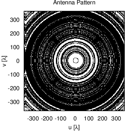
Figure 1.— Coverage pattern (black) in the $uv$-plane. This pattern results from selecting all baseline pairs from 20 randomly-placed antennas pointed at a celestial pole. The pattern is then rotated uniformly on the same patch of sky for $12$ hr.

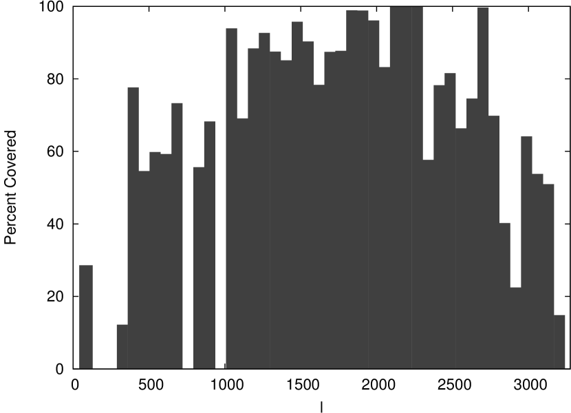
Figure 2.— Antenna coverage for each $\ell$-bin. Shown is the percentage of cells within the annulus defined by the radius $\ell$ intersected by any antenna during the $12$ hr observation period.

We determine the noise per pixel by summing the integration time spent in that pixel by all baselines. We do not adopt a noise model for a particular instrument; rather, we set the noise variance to be $\sigma_{i}^{2}\propto 1/t_{{\rm obs},i}$. We then set an overall signal-to-noise ratio of $10$ by multiplying all noise variances by a constant value to maintain $|IFA~{}s|/|In|=10$. This provides a scaling of the noise that would normally be caused by instrument effects such as the surface area of the detectors and the system temperature in a realistic observation. We use a Gaussian realization of this noise to create the data in Equation (1). We show the process going from input signal to data $d$ in Figure 3.

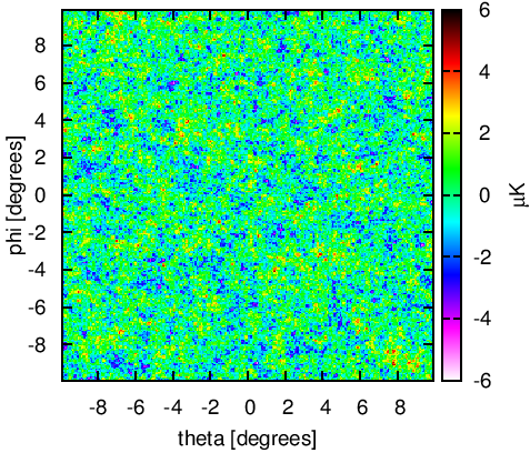
(a) Input Sky ($s$)

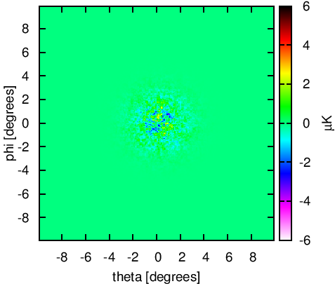
(b) Beam Application ($A~{}s$)

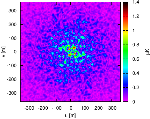
(c) Fourier Transform ($FA~{}s$)

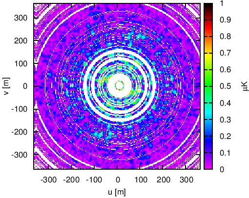
(d) Interferometer Application ($IFA~{}s$)

(e) Data ($IFA~{}s+I~{}n$)

Figure 3.— Observation-making process. Shown are (a) the input sky signal $s$, (b) the application of a primary beam, which we model as a Gaussian with standard deviation $1.5$ deg, (c) Fourier transformation onto the $uv$-plane, (d) application of $20$ randomly placed antennas rotated uniformly for 12 hr, and (e) the addition of the noise. Note that all images in the $uv$-plane are shown as magnitudes.

3.1. Computational Considerations and Correlation between Samples

The computational complexity of the Gibbs sampling algorithm as applied to single-dish experiments has been discussed in detail in previous works (e.g., Wandelt et al. 2004) where it was shown that the scaling is dominated by spherical harmonic transforms, which scale as $\mathcal{O}(\ell^{3})$. Since we are dealing with small patches on the sky, assume that all horns have identical beams, and discretize the $uv$-plane, the analysis time is dominated by two-dimensional fast Fourier transforms, which scale as $\mathcal{O}(\ell^{2}\log{\ell})$.

The scaling estimate concerns the time to compute individual samples. The total time required to perform a full analysis also depends on the number of samples required for a satisfactory exploration of the Bayesian posterior density. For single-dish experiments the correlation length for individual $C_{\ell}$ bins can become large for high $\ell$ where many modes with individually low signal-to-noise combine together. This can lead to very long convergence times and limited scalability, which requires special tricks for the analysis of low signal-to-noise regimes as described in Jewell et al. (2009). As we will see, however, compact antenna arrays result in an approximately uniform coverage of the $uv$-plane. The correlation length is a function of coverage and therefore we obtain approximately uniform signal-to-noise as a function of $\ell$ which means the correlation function will be a weak function of $\ell$.

We ran four independent Gibbs sampler chains for $2000$ iterations each. We discarded the first $1000$ iterations for a “burn-in” phase. After this number of iterations, the G-R statistic reached less than $1.1$ for all bins. This analysis took roughly 75 hr on 4 cores of an Intel dual six-core X5650 Westmere 2.66GHz machine and consumed only 10 MB of memory. We show in Figure 4 the number of steps required to satisfy our G-R convergence criterion versus the sky coverage percentage for each $\ell$-bin. Shown are the number of steps after the burn-in phase.

We see little correlation between $uv$-plane coverage and time to convergence. As we will see in the power spectrum results below, reduced coverage does lead to a variable correlation length (larger for small power and shorter for large power). This means that some low-coverage bins dominate our convergence rate and hence overall performance. This is a consequence of the ratio of the size of the Gibbs move to the full width of the posterior (Eriksen et al. 2004).

Large correlation lengths, which lead to longer convergence times, do not have a large impact on the feasibility of the example analysis we present here; however, they would be more important in the limit where detector noise is large compared to the observed signal (e.g., if the goal was to place upper limits on an as-yet unobserved signal, as is currently the case with inflationary B-mode missions). This issue will therefore have to be revisited for polarization data. In any case, if long correlation lengths in the Markov chain were to cause poor performance, we could follow the general prescription of Jewell et al. (2009) by incorporating a step with a Metropolis-Hastings sampler and deterministic rescaling of the sky signal.

Figure 4.— Number of steps after burn-in required to satisfy the G-R convergence criterion versus the sky coverage percentage for each $\ell$-bin.

4. Results

4.1. Power Spectrum

In Figure 5 we show the mean posterior angular power spectrum of the of the four independent chains after reaching convergence. We also show the uncertainty associated with each $\ell$-bin and the corresponding power of our input signal realization. The size of the uncertainties in each bin are consistent with varying coverage in the $uv$-plane; i.e., those bins with little to no coverage have correspondingly large error bars, while those bins with complete coverage have the tightest constraints. All of our estimates fall within $2\sigma$ of the expected value, and most within $1\sigma$, as expected with this number of bins.

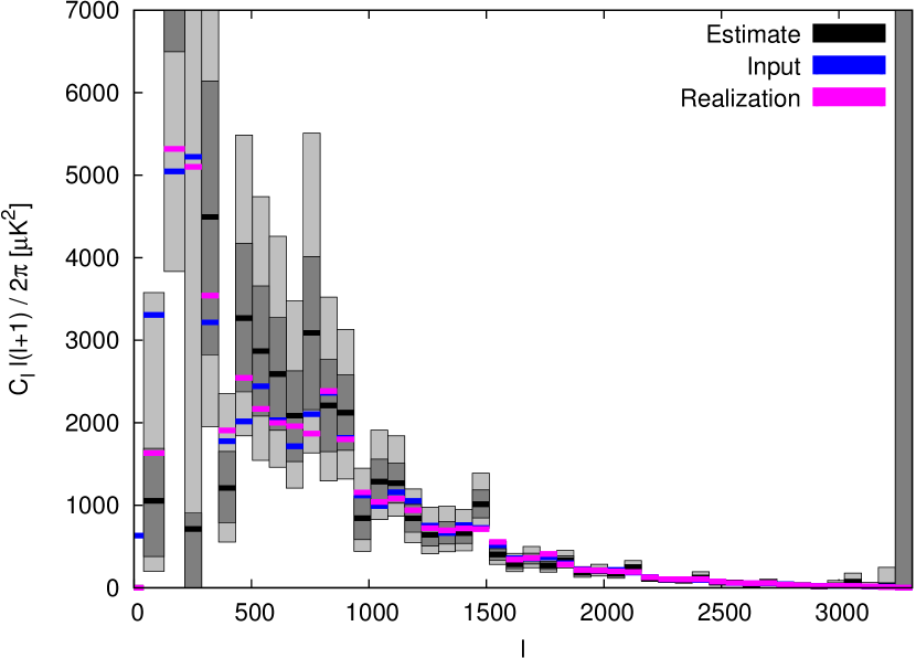
Figure 5.— Mean posterior angular power spectrum for each $\ell$-bin (black) with $1\sigma$ (dark gray) and $2\sigma$ (light gray) uncertainties. The binned input CMB angular power spectrum is shown in blue and the angular power spectrum of our specific signal realization is shown in pink.

Figure 6 shows individual marginalized probability densities for a selection of $\ell$-bin. We immediately note the shape of each probability distribution matches qualitatively that of an inverse gamma distribution, as expected. We see the damaging effects of the lack of $uv$-plane coverage especially in the case of $\ell\sim 300$. Here, the lack of any input signal leads to a uniformly decreasing posterior probability density function (pdf) with a very long power-law tail to large power. This can be summarized as an upper bound on the power in that bin. In other bins, slightly reduced coverage combined with the effects of noise yields wide and noisy distributions.

Figure 6.— Histograms of marginalized probability densities for a selection of $\ell$-bins with varying levels of $uv$-plane coverage (see Figure 2). Note that all samples outside of the plotted range are collected in the edge bins.

Beyond the marginalized posteriors for each angular power spectrum bin amplitude, the posterior samples also contain higher-order information. Figure 7 shows the two-point correlations between all pairs of angular power spectrum bins. For this plot, we suppress the diagonal components so that we can more easily examine the cross-bin correlations. While the correlation matrix is somewhat noisy, we immediately see the effects of the reduced sky coverage due to a finite beam width as correlations between adjacent modes. This beam leads to reduced Fourier space resolution. The correlation data are informative about regions of the signal data $d$ which are larger than a single angular power spectrum bin. This slight oversampling of the power leads to a tendency of bins to be anti-correlated with each other. Anti-correlation occurs because data constrain power in regions of the signal and if a particular bin scatters high, the inference in adjacent bins reduces in power to remain consistent with the data (Elsner & Wandelt 2012).

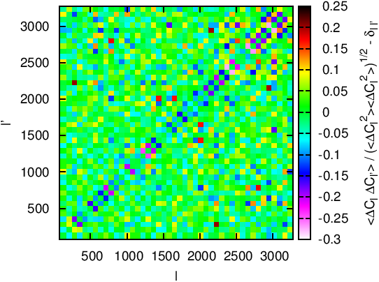
Figure 7.— Power spectrum correlation matrix. Shown are the correlations between all pairs of angular power spectrum bins. Diagonal elements are suppressed to enhance the visibility of off-diagonal correlations. This matrix highlights the mode coupling due to the beam as correlations between adjacent bins. We also see slight (anti-)correlations of adjacent angular power spectrum bins due to discrete sampling of the angular power spectrum.

4.2. Signal Reconstruction

Figure 8 shows several sample posterior maps (i.e., the solution $s^{i+1}$ to Equation 4). We show the signal samples at steps 0 and 1000 after the “burn-in” phase. The Gibbs sampler fills in the map outside of the primary beam with fluctuations consistent with the actual data. While maps made from interferometric data are often accompanied by an “effective beam”, each signal sample presented here has no smoothing. The signal samples are a population of possible pure signal skies which are consistent with the data.

(a) Signal Sample, Iteration 0

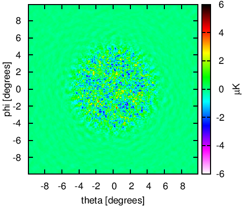
(b) Wiener-Filtered Signal, Iteration 0

(c) Signal Sample, Iteration 1000

(d) Wiener-Filtered Signal, Iteration 1000

Figure 8.— Posterior signal samples at various stages of the Gibbs sampling algorithm. Shown are (a) signal sample with fluctuations at step 0 after the burn-in phase, (b) Wiener-filtered map at step 0 after the burn-in phase, (c) signal sample with fluctuations at step 1000, and (d) Wiener-filtered map at step 1000.

We can also easily compute Wiener-filtered maps: setting the fluctuation vectors $\xi_{1}=\xi_{2}=0$ in Equation (4) and solving for $s^{i+1}$ provides the definition of a Wiener-filtered map (Wandelt et al. 2004). We show these maps for iterations 0 and 1000 also in Figure 8. The Wiener filter adaptively smooths the map depending on the data support. In this case, the filter eliminates the fluctuations outside of the primary beam, where there is no data, and successfully recovers the signal in the observed region.

After sufficient iterations the artificially created fluctuations average out and we are left with a reliable reconstruction of the input signal within the area of the primary beam, which we show in Figure 9. We accompany this final mean posterior signal map with the “dirty” map, which is $F^{-1}(IAF~{}s+In)$. Note that the dirty map contains artifacts such as grating rings and sidelobes which are absent from our posterior map. Also, the dirty map completely misses the strongest fluctuations.

(a) Dirty Map

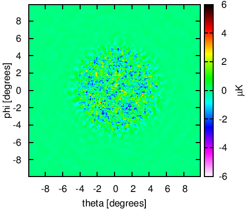
(b) Final Mean Posterior Map

Figure 9.— Final map reconstructions. Shown are the “dirty” map $F^{-1}(IAF~{}s+n)$ divided by the beam response (a). and the final mean posterior signal map (b). We have limited the beam to 1% of its maximum value for clarity.

We show the difference between the final mean posterior signal map to the input map in Figure 10. We see that medium-scale fluctuations remain; however, the amplitude of these fluctuations are below the typical scale of fluctuations in the input signal and are consistent with the uncertainties in the median-$\ell$ reconstructed power spectrum (Figure 5), which are caused by incomplete $uv$-plane coverage. Outside the beam our final posterior map is nearly zero (as desired), leading to a reconstruction of the input map in the residual.

Figure 10.— Final map residual: shown is the difference between the final mean posterior signal map and the input map.

5. Conclusion

We have successfully demonstrated the technique of Gibbs sampling as applied to interferometric observations. Our approach accounts for realistic interferometer features, such as baseline-dependent noise, mode coupling due to a finite beam size, and incomplete coverage of the $uv$-plane. We have presented an example of CMB angular power spectrum estimation and signal reconstruction of a moderately large ($n_{p}=256^{2}$) mock data set directly applicable to current and near-future missions.

A complete interferometric analysis tool for a realistic future mission must include several features not studied here: multiple frequencies, polarization (Chiueh & Ma 2002), mosaicking (Bunn & White 2007), a true spherical sky (Bunn & White 2008), and wide bandwidths (Subrahmanyan 2004). Building a complete pipeline is beyond the scope of the present study which focused on the ability of Gibbs sampling to explore the full shape of the joint, multivariate, non-Gaussian posterior pdf for the angular power spectrum and the signal map given the data.

Within the Bayesian framework, strictly speaking, angular power spectrum estimation only makes sense if Gaussianity and statistical isotropy is assumed. An isotropic Gaussian process prior is a highly accurate model of the CMB anisotropies and therefore the detailed shape of the derived angular power spectrum posterior is of great physical interest for that application.

While we have focused our example on CMB observations, our basic technique can be generalized to a wide variety of interferometer observations, such as the planned study of the 21 cm signal from the epoch of reionization (Morales & Hewitt 2004), which can provide useful constraints on cosmological parameters (McQuinn et al. 2006). In applications to non-CMB data sets the Gaussian process prior may not strictly hold, but can be motivated from a maximum entropy argument: given only a model of the mean and covariance (defined by the angular power spectrum) of a data set, the least informative completion to a full probabilistic model yields a Gaussian process prior. In that case the method still maps out the angular power spectrum likelihood taking into account all modeled signals and imperfections in the data at the two-point correlation level.

In the derivation of the Gibbs sampling method using the conditional densities of the posterior distribution, the signal angular power spectrum samples are paired with optimal (minimum-variance) signal reconstructions assuming that same power spectrum. Averaged along the chain the algorithm therefore simultaneously discovers the correlation structure in the data, reconstructs optimal sky maps, and explores the range of uncertainty left by having finite amounts of imperfect data. The mean posterior signal reconstruction can be viewed as a non-linear generalization of the least-squares optimal signal reconstruction provided by the Wiener filter without requiring an a priori choice of the signal covariance.

In any case, the assumption of statistical isotropy in the covariance model still holds in a standard FRW cosmology even for applications to 21 cm data on any given redshift slice. To tackle such a difficult analysis, our Gibbs sampling approach must be extended to deal with the significant galactic and extragalactic foregrounds present (Santos et al. 2005; Furlanetto et al. 2006; Bernardi et al. 2009; Liu & Tegmark 2012) and to include in the solution the full three spatial dimensions of the data and frequency dependence of the angular power spectrum.

By extending the Gibbs sampling framework to interferometric observations, we have demonstrated the validity of this method in this regime and its power in providing computationally efficient $\mathcal{O}(n_{p}\log n_{p})$ angular power spectrum analysis and signal reconstruction. Our method is able to fully explore the angular power spectrum likelihood shape in an optimal fashion. However, even with this scaling extremely large data sets can still take weeks to analyze with a single machine. Fortunately there are many opportunities for parallelism. For example, independent chains can be run as separate execution threads in a straightforward manner. Also, we developed our code with the open-source PETSc library  (Balay et al. 1997, 2010, 2011) and the MPI-parallelized version of FFTW (Frigo & Johnson 2005), meaning that maps can be divided up among multiple processors with communication handled by the internal libraries. This Bayesian framework can therefore plausibly cope with the extreme data analysis requirements of future CMB or 21 cm missions.

References

- Balay et al. (1997) Balay, S., Gropp, W. D., McInnes, L. C., & Smith, B. F. 1997, in Modern Software Tools in Scientific Computing, ed. E. Arge, A. M. Bruaset, & H. P. Langtangen (Birkh{ä}user Press), 163–202
- Balay et al. (2010) Balay, S. et al. 2010, PETSc Users Manual, Tech. Rep. ANL-95/11 - Revision 3.1, Argonne National Laboratory
- Balay et al. (2011) —. 2011, PETSc Web page
- Benabed et al. (2009) Benabed, K., Cardoso, J.-F., Prunet, S., & Hivon, E. 2009, MNRAS, 400, 219
- Bernardi et al. (2009) Bernardi, G. et al. 2009, A&A, 500, 965
- Booth et al. (2009) Booth, R. S., de Blok, W. J. G., Jonas, J. L., & Fanaroff, B. 2009, ArXiv e-prints: 0910.2935
- Bunn & White (2007) Bunn, E. F. & White, M. 2007, ApJ, 655, 21
- Bunn & White (2008) Bunn, E. F. & White, M. 2008, in Bulletin of the American Astronomical Society, Vol. 40, American Astronomical Society Meeting Abstracts #212, 221
- Cantalupo et al. (2010) Cantalupo, C. M., Borrill, J. D., Jaffe, A. H., Kisner, T. S., & Stompor, R. 2010, ApJS, 187, 212
- Chiueh & Ma (2002) Chiueh, T. & Ma, C. 2002, ApJ, 578, 12
- Chu et al. (2005) Chu, M., Eriksen, H. K., Knox, L., Górski, K. M., Jewell, J. B., Larson, D. L., O’Dwyer, I. J., & Wandelt, B. D. 2005, Phys. Rev. D, 71, 103002
- Dickinson et al. (2004) Dickinson, C. et al. 2004, MNRAS, 353, 732
- Dickinson et al. (2009) —. 2009, ApJ, 705, 1607
- Elsner & Wandelt (2012) Elsner, F. & Wandelt, B. D. 2012, A&A, 542, A60
- Eriksen et al. (2004) Eriksen, H. et al. 2004, ApJS, 155, 227
- Eriksen et al. (2007) Eriksen, H. K., Huey, G., Banday, A. J., Górski, K. M., Jewell, J. B., O’Dwyer, I. J., & Wandelt, B. D. 2007, ApJ, 665, L1
- Faÿ et al. (2008) Faÿ, G., Guilloux, F., Betoule, M., Cardoso, J.-F., Delabrouille, J., & Le Jeune, M. 2008, Phys. Rev. D, 78, 083013
- Frigo & Johnson (2005) Frigo, M. & Johnson, S. 2005, Proceedings of the IEEE, 93, 216
- Furlanetto et al. (2006) Furlanetto, S. R., Oh, S. P., & Briggs, F. H. 2006, Phys. Rep., 433, 181
- Gelman & Rubin (1992) Gelman, A. & Rubin, D. 1992, Statistical Science, 7, 457
- Grainge et al. (2003) Grainge, K. et al. 2003, MNRAS, 341, L23
- Halverson et al. (2002) Halverson, N. W. et al. 2002, ApJ, 568, 38
- Hauser & Peebles (1973) Hauser, M. G. & Peebles, P. J. E. 1973, ApJ, 185, 757
- Hivon et al. (2002) Hivon, E., Górski, K. M., Netterfield, C. B., Crill, B. P., Prunet, S., & Hansen, F. 2002, ApJ, 567, 2
- Hobson & Maisinger (2002) Hobson, M. P. & Maisinger, K. 2002, MNRAS, 334, 569
- Jarvis (2007) Jarvis, M. J. 2007, At the Edge of the Universe: Latest Results from the Deepest Astronomical Surveys ASP Conference Series, 380
- Jasche et al. (2010) Jasche, J., Kitaura, F. S., Wandelt, B. D., & Enßlin, T. A. 2010, MNRAS, 406, 60
- Jasche & Wandelt (2012) Jasche, J. & Wandelt, B. D. 2012, MNRAS, 3469
- Jewell et al. (2004) Jewell, J., Levin, S., & Anderson, C. H. 2004, ApJ, 609, 1
- Jewell et al. (2009) Jewell, J. B., Eriksen, H. K., Wandelt, B. D., O’Dwyer, I. J., Huey, G., & Górski, K. M. 2009, ApJ, 697, 258
- Johnston et al. (2008) Johnston, S. et al. 2008, Experimental Astronomy, 22, 151
- Kitaura & Enßlin (2008) Kitaura, F. S. & Enßlin, T. A. 2008, MNRAS, 389, 497
- Kitaura et al. (2010) Kitaura, F.-S., Gallerani, S., & Ferrara, A. 2010, ArXiv e-prints: 1011.6233
- Komatsu et al. (2011) Komatsu, E. et al. 2011, ApJS, 192, 18
- Kovac et al. (2002) Kovac, J. M., Leitch, E. M., Pryke, C., Carlstrom, J. E., Halverson, N. W., & Holzapfel, W. L. 2002, Nature, 420, 772
- Larson et al. (2011) Larson, D. et al. 2011, ApJS, 192, 16
- Larson et al. (2007) Larson, D. L., Eriksen, H. K., Wandelt, B. D., Górski, K. M., Huey, G., Jewell, J. B., & O’Dwyer, I. J. 2007, ApJ, 656, 653
- Leitch et al. (2002) Leitch, E. M. et al. 2002, ApJ, 568, 28
- Lewis et al. (2000) Lewis, A., Challinor, A., & Lasenby, A. 2000, ApJ, 538, 473
- Lidz et al. (2008) Lidz, A., Zahn, O., McQuinn, M., Zaldarriaga, M., & Hernquist, L. 2008, ApJ, 680, 962
- Liu & Tegmark (2012) Liu, A. & Tegmark, M. 2012, MNRAS, 419, 3491
- Lonsdale et al. (2009) Lonsdale, C. J. et al. 2009, Proceedings of the IEEE, 97, 1497
- Mason et al. (2003) Mason, B. S. et al. 2003, ApJ, 591, 540
- McQuinn et al. (2006) McQuinn, M., Zahn, O., Zaldarriaga, M., Hernquist, L., & Furlanetto, S. R. 2006, ApJ, 653, 815
- Morales & Hewitt (2004) Morales, M. F. & Hewitt, J. 2004, ApJ, 615, 7
- Myers et al. (2006) Myers, S. et al. 2006, New Astronomy Reviews, 50, 951
- Myers et al. (2003) Myers, S. T. et al. 2003, ApJ, 591, 575
- O’Dwyer et al. (2004) O’Dwyer, I. J., Eriksen, H. K., Wandelt, B. D., Jewell, J. B., Larson, D. L., Górski, K. M., Banday, A. J., Levin, S., & Lilje, P. B. 2004, ApJ, 617, L99
- Park et al. (2003) Park, C., Ng, K., Park, C., Liu, G., & Umetsu, K. 2003, ApJ, 589, 67
- Parsons et al. (2008) Parsons, A. et al. 2008, Publications of the Astronomical Society of the Pacific, 120, 1207
- Parsons et al. (2010) Parsons, A. R. et al. 2010, AJ, 139, 1468
- Pearson et al. (2000) Pearson, T. J. et al. 2000, eprint arXiv:astro-ph/0012212
- Press et al. (1986) Press, W. H., Flannery, Brian P., & Teukolsky, Saul A. 1986, Cambridge: University Press
- Readhead et al. (2004) Readhead, A. C. S. et al. 2004, Science (New York, N.Y.), 306, 836
- Rybicki & Press (1992) Rybicki, G. B. & Press, W. H. 1992, ApJ, 398, 169
- Santos et al. (2005) Santos, M. G., Cooray, A., & Knox, L. 2005, ApJ, 625, 575
- Sharp et al. (2010) Sharp, M. K. et al. 2010, ApJ, 713, 82
- Sievers & CBI Collaboration (2005) Sievers, J. & CBI Collaboration. 2005, in Bulletin of the American Astronomical Society, Vol. 37, American Astronomical Society Meeting Abstracts, 100.07
- Sievers et al. (2009) Sievers, J. L. et al. 2009, eprint arXiv:0901.4540
- Subrahmanyan (2004) Subrahmanyan, R. 2004, MNRAS, 348, 1208
- Subrahmanyan & Ekers (2002) Subrahmanyan, R. & Ekers, R. D. 2002, eprint arXiv:astro-ph/0209569
- Sutton & Wandelt (2006) Sutton, E. C. & Wandelt, B. D. 2006, ApJS, 162, 401
- Szapudi et al. (2001) Szapudi, I., Prunet, S., Pogosyan, D., Szalay, A. S., & Bond, J. R. 2001, ApJ, 548, L115
- Taylor et al. (2008a) Taylor, J. F., Ashdown, M. A. J., & Hobson, M. P. 2008a, MNRAS, 389, 1284
- Taylor et al. (2008b) —. 2008b, MNRAS, 389, 1284
- Tegmark (1997) Tegmark, M. 1997, Phys. Rev. D, 55, 5895
- Thompson et al. (2001) Thompson, A. R., Moran, J. M., & Swenson, George W., J. 2001, Interferometry and synthesis in radio astronomy by A. Richard Thompson
- Timbie & Tucker (2009) Timbie, P. T. & Tucker, G. S. 2009, Journal of Physics: Conference Series, 155, 012003
- Tristram & Ganga (2007) Tristram, M. & Ganga, K. 2007, Reports on Progress in Physics, 70, 899
- Wandelt et al. (2004) Wandelt, B., Larson, D., & Lakshminarayanan, A. 2004, Phys. Rev. D, 70, 12
- Wandelt et al. (2001) Wandelt, B. D., Hivon, E., & Górski, K. M. 2001, Phys. Rev. D, 64, 083003
- White et al. (1999) White, M., Carlstrom, J. E., Dragovan, M., & Holzapfel, W. L. 1999, ApJ, 514, 12