Collisions between Gravity-Dominated Bodies:
2. The Diversity of Impact Outcomes during the End Stage of Planet Formation

Abstract

Numerical simulations of the stochastic end stage of planet formation typically begin with a population of embryos and planetesimals that grow into planets by merging. We analyzed the impact parameters of collisions leading to the growth of terrestrial planets from recent $N$-body simulations that assumed perfect merging and calculated more realistic outcomes using a new analytic collision physics model. We find that collision outcomes are diverse and span all possible regimes: hit-and-run, merging, partial accretion, partial erosion, and catastrophic disruption. The primary outcomes of giant impacts between planetary embryos are approximately evenly split between partial accretion, graze-and-merge, and hit-and-run events. To explore the cumulative effects of more realistic collision outcomes, we modeled the growth of individual planets with a Monte Carlo technique using the distribution of impact parameters from $N$-body simulations. We find that fewer planets reached masses $>0.7M_{\rm Earth}$ using the collision physics model compared to simulations that assumed every collision results in perfect merging. For final planets with masses $>0.7M_{\rm Earth}$, 60% are enriched in their core-to-mantle mass fraction by $>10$% compared to the initial embryo composition. Fragmentation during planet formation produces significant debris ($\sim 15$% of the final mass) and occurs primarily by erosion of the smaller body in partial accretion and hit-and-run events. In partial accretion events, the target body grows by preferentially accreting the iron core of the projectile and the escaping fragments are derived primarily from the silicate mantles of both bodies. Thus, the bulk composition of a planet can evolve via stochastic giant impacts.

1. Introduction

The end stage of terrestrial planet formation is defined by the final competition between planetary embryos as they grow via collisions into a final set of stable planets (e.g., Chambers, 2004). The last giant impact is invoked to explain major differences between the solid planets in our Solar System. The large core mass fraction for Mercury could be the result of a single mantle-stripping impact event (Benz et al., 2007). A planet’s spin orientation and period is strongly influenced by the last giant impact (Lissauer, 1993). Giant collisions are also invoked to explain the formation of Earth’s moon (Canup & Asphaug, 2001), the Pluto system (Canup, 2005), and the Haumea system (Leinhardt et al., 2010).

The growth of planetary embryos into planets is commonly modeled using $N$-body techniques in order to capture the details of the multiple gravitational interactions. Because typical encounter velocities between embryos are in the range of 1 to 3 mutual escape velocities (e.g., Agnor et al., 1999), almost all $N$-body simulations have assumed that the two colliding embryos merge into a single body with the same total mass. However, hydrocode simulations of oblique collisions between embryos found that inelastic collisions, known as hit-and-run (H&R) events (Agnor & Asphaug, 2004; Asphaug et al., 2006), are a common outcome at speeds just above the mutual escape velocity. Asphaug (2010) estimated that about half of giant impacts are hit-and-run events. The physics of giant impacts is sufficiently complicated that the impact parameters demarcating the transition between merging and hit-and-run outcomes was defined only recently by an empirical analysis of over a thousand hydrocode impact simulations (Kokubo & Genda, 2010; Genda et al., 2012).

Collision outcomes other than merging and hit-and-run are possible during planet formation. The range of outcomes include partial accretion, partial erosion, and catastrophically disruptive events. Some planet formation simulations, focusing on specific stages of planet growth, have directly modeled each encounter between two bodies in order to capture the details of the collision physics (Genda et al., 2011; Leinhardt & Richardson, 2005; Leinhardt et al., 2009), but this approach is too computationally expensive to be widely adopted. To date, planet formation studies have not had access to a robust collision physics model that could be implemented easily into $N$-body simulations.

In a companion paper (Leinhardt & Stewart, 2012), we have developed a comprehensive analytic model to predict the outcome of any collision between gravity-dominated bodies. The model predicts the transitions between collision regimes and the size and velocity distribution of fragments. Collision outcomes depend on the projectile-to-target mass ratio, impact angle, impact velocity, and two material parameters that define the catastrophic disruption criteria. Catastrophic disruption is defined by the specific impact energy needed to disperse half the total mass. For collisions that result in partial accretion or erosion of differentiated bodies, we estimate the change in the core-mantle mass ratio following the work of Marcus et al. (2009, 2010). The new analytic model now allows planet formation simulations to capture the full diversity of collision outcomes.

To assess the effects of including more realistic collision physics in planet formation studies, we analyzed the impact parameters from recent $N$-body simulations of terrestrial planet formation that assumed perfect merging and calculated the more realistic collision outcomes (O’Brien et al., 2006; Raymond et al., 2009). The results provide insights into the most important collision regimes, quantify the probabilities of different outcomes, and identify future challenges in planet formation simulations.

Then, using the distribution of impact parameters from the $N$-body simulations, we modeled individual planet growth with a Monte Carlo technique in order to assess the cumulative effects of diverse collision outcomes. We compare the distribution of final planet masses from simulations with different assumptions about collision outcomes and tracked changes in the core mass fraction. The collision physics model allows for more detailed investigation of the evolution of the bulk chemistry and for tighter isotopic constraints on terrestrial planet formation studies.

2. The Collision Outcome Model

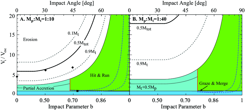
Figure 1.— Predicted collision outcome maps using the analytic model for strengthless planets (with material parameters $c^{*}=1.9$ and $\bar{\mu}=0.36$) for two projectile-to-target mass ratios of (A) $M_{\rm p}:M_{\rm t}=1:10$ and (B) 1:40. Impact velocity is normalized by the mutual surface escape velocity; impact parameter is spaced according to probability. Colored regions denote perfect merging (dark blue), partial accretion to the target (medium blue), net erosion to the target (white), hit-and-run (green), and graze-and-merge (blue-green). Vertical red line at $b_{\rm crit}$ denotes the transition between non-grazing and grazing events. Thick black curve – critical velocity for catastrophic disruption; dashed grey curves – 10% and 90% of target mass in largest remnant; dotted black curve – 50% of projectile accreted; dot-dashed blue curve – catastrophic disruption of the projectile in a hit-and-run; dashed blue curve – onset of erosion of projectile in a hit-and-run. Symbols denote proposed giant impact events: $\blacklozenge$ – Mercury (Benz et al., 2007); $\blacksquare$ – Earth-Moon (Canup, 2004).

The outcome of a collision in the gravity regime was predicted using the new analytic collision physics model from Leinhardt & Stewart (2012), hereafter LS12. The model is summarized here; refer to LS12 for the full details and limitations. In the gravity regime, erosive outcomes are primarily controlled by overcoming gravitational forces rather than overcoming material strength; bodies larger than about 100 to 1000 m in size are dominated by gravity (e.g., Melosh & Ryan, 1997). The model predicts the collision outcome as a function of projectile-to-target mass ratio ($\gamma=M_{\rm p}/M_{\rm t}$), impact angle ($\theta$), and impact velocity ($V_{i}$). By convention, the projectile is less massive than the target ($M_{\rm p}\leq M_{\rm t}$). The following equations were used to generate the boundaries and contours on the example collision outcome maps shown in Figure 1.

Partial accretion and erosive outcomes are defined by the catastrophic disruption criteria ($Q^{*}_{RD}$), which is the specific impact energy required to disrupt and gravitationally disperse half the total mass. For a particular collision, the total specific impact energy in the center of mass frame is given by

$$Q_{R}=\frac{\mu V_{i}^{2}}{2M_{\rm tot}},$$ (1)

where $M_{\rm tot}=M_{\rm p}+M_{\rm t}$ and $\mu=M_{\rm p}M_{\rm t}/M_{\rm tot}$ is the reduced mass. For bodies in the gravity regime, the head-on disruption criteria increases with increasing mass and follows the general form derived by Housen & Holsapple (1990):

$$Q^{*}_{RD}=q_{g}\left(\rho_{1}G\right)^{3\bar{\mu}/2}R_{C1}^{3\bar{\mu}}V^{*(2-3\bar{\mu})},$$ (2)

where $R_{C1}$ is the spherical radius of the combined projectile and target masses at a density of $\rho_{1}\equiv 1000$ kg m^-3 and $G$ is the gravitational constant. At the critical impact velocity $(V_{i}=V^{*})$, the specific impact energy is equal to the catastrophic disruption threshold $(Q_{R}=Q^{*}_{RD})$ for the particular impact scenario ($R_{C1}$ and mass ratio). Instead of target radius, the variable $R_{C1}$ was introduced by Stewart & Leinhardt (2009) in order to generalize the dependence of $Q^{*}_{RD}$ on size for different density bodies and for different projectile-to-target mass ratios. The coefficient $q_{g}$ is of order 1 and defined below. $\bar{\mu}$ is the velocity exponent in the point source coupling parameter from Housen & Holsapple (1990). LS12 fit a value of $\bar{\mu}=0.36\pm 0.01$ using the results from several numerical studies of disruption in the gravity regime on a wide variety of materials (weak rock, ice, rubble piles).

LS12 derived the disruption criteria for a reference case of a head-on impact between two equal-mass bodies, which represents the minimum energy scenario to disrupt a particular target. The critical impact velocity for head-on equal mass collisions is given by

$$V^{*}_{\gamma=1}=\left(\frac{32\pi c^{*}}{5}\right)^{1/2}(\rho_{1}G)^{1/2}R_{C1},$$ (3)

where $c^{*}$ is a nondimensional material parameter that is fitted to simulation data. LS12 fit $c^{*}=1.9\pm 0.3$ for fluid planets and $c^{*}=5\pm 2$ for various solid planetesimal analogs using the results from several numerical studies. $c^{*}$ is defined such that it represents the value of the equal-mass head-on disruption criteria in units of the specific gravitational binding energy of the combined mass:

$$Q^{*}_{RD,\gamma=1}=c^{*}\frac{4}{5}\pi\rho_{1}GR_{C1}^{2}.$$ (4)

Equation 4 is named the “principal disruption curve.” Combining the previous equations gives the coefficient for Equation 2:

$$q_{g}=\frac{1}{8}\left(\frac{32\pi c^{*}}{5}\right)^{3\bar{\mu}/2}.$$ (5)

The derivation of Equation 2 assumed that all of the projectile’s kinetic energy is deposited in the target. This assumption is often invalid as a portion of the projectile misses the target for many combinations of projectile-to-target mass ratio and impact angle. For an oblique impact, LS12 derived the mass fraction of the projectile that geometrically overlaps with the target,

$$\alpha=\begin{cases}1&\text{if $R_{\rm t}>b(R_{\rm p}+R_{\rm t})+R_{\rm p}$,}\\ \rho(\pi R_{\rm p}l^{2}-\pi l^{3}/3)&\text{otherwise,}\end{cases}$$ (6)

where $\rho$ is the density of the projectile, $b=\sin\theta$ is the impact parameter ($b=0$ for head-on impacts) and $l/(2R_{\rm p})$ is the fraction of the projectile diameter that overlaps the target. The impact angle and overlapping mass fraction are defined at the point of first contact assuming spherical bodies. Using just the interacting fraction the projectile, the angle-adjusted reduced mass is

$$\mu_{\alpha}=\frac{\alpha M_{\rm p}M_{\rm t}}{\alpha M_{\rm p}+M_{\rm t}}.$$ (7)

The disruption criteria and critical impact velocity for a specific mass ratio and impact angle are calculated by adjustments to the head-on equal-mass principal disruption curve. To achieve disruption with a smaller projectile, the impact velocity rises to

$$V^{*}=\left[\frac{1}{4}\frac{(\gamma+1)^{2}}{\gamma}\right]^{1/(3\bar{\mu})}V^{*}_{\gamma=1},$$ (8)

and, from Equation 2, the catastrophic disruption criteria increases by

$$Q^{*}_{RD} = Q^{*}_{RD,\gamma=1}\left(\frac{V^{*}}{V^{*}_{\gamma=1}}\right)^{2-3\bar{\mu}},$$ (9)

$$= Q^{*}_{RD,\gamma=1}\left[\frac{1}{4}\frac{(\gamma+1)^{2}}{\gamma}\right]^{2/(3\bar{\mu})-1}.$$

Next, accounting for the projectile interacting mass fraction for oblique impacts,

$$Q^{\prime*}_{RD}=\left(\frac{\mu}{\mu_{\alpha}}\right)^{2-3\bar{\mu}/2}Q^{*}_{RD},$$ (10)

where the prime notation indicates the value for an oblique impact. Finally, from Equation 1, the critical impact velocity adjusted for both the mass ratio and impact angle is

$$V^{\prime*}=\sqrt{2Q^{\prime*}_{RD}M_{\rm tot}/\mu}.$$ (11)

The equations for $Q^{\prime*}_{RD}$ and $V^{\prime*}$ are curves as a function of $R_{C1}$, impact angle (within $\mu_{\alpha}$), mass ratio (within $\mu$), and two material parameters, $c^{*}$ and $\bar{\mu}$.

The specific collision outcome regime is determined using the mutual escape velocity, disruption criteria, and impact parameter. When the impact velocity is below the mutual escape velocity of the interacting mass ($M^{\prime}_{\rm tot}=\alpha M_{\rm p}+M_{\rm t}$), the two bodies are assumed to merge completely (perfect merging). Above $V^{\prime}_{\rm esc}=\sqrt{2GM^{\prime}_{\rm tot}/(R_{\rm p}+R_{\rm t})}$, the collisions outcomes are divided into two groups: grazing and non-grazing.

The transition between non-grazing and grazing outcomes is demarcated by a critical impact parameter, $b_{\rm crit}$. Following Asphaug (2010), the center of the projectile is tangent to the target at the critical impact parameter,

$$b_{\rm crit}=\left(\frac{R}{R+r}\right).$$ (12)

Non-grazing ($b<b_{\rm crit}$) collisions transition from perfect merging to the disruption regime with increasing impact velocity. In the disruption regime, the outcome may be partial accretion or partial erosion depending on the mass of the largest remnant, $M_{\rm lr}$. The largest remnant mass is calculated using the impact energy and the catastrophic disruption criteria. For collisions with $0<Q_{R}/Q^{\prime*}_{RD}<1.8$, $M_{\rm lr}$ is proportional to impact energy:

$$\frac{M_{\rm lr}}{M_{\rm tot}}=-0.5\left(\frac{Q_{R}}{Q^{\prime*}_{RD}}-1\right)+0.5.$$ (13)

Because a single line fit a wide variety of simulation results, we named this linear relationship the “universal law for the mass of the largest remnant” (Stewart & Leinhardt, 2009). In the case of super-catastrophic disruption, $Q_{R}/Q^{\prime*}_{RD}\geq 1.8$, the largest remnant follows a power law,

$$\frac{M_{\rm lr}}{M_{\rm tot}}=\frac{0.1}{1.8^{\eta}}\left(\frac{Q_{R}}{Q^{\prime*}_{RD}}\right)^{\eta},$$ (14)

where $\eta\sim-1.5$ based on laboratory disruption experiments, as discussed in LS12.

Grazing ($b>b_{\rm crit}$) collisions transition from perfect merging to a graze-and-merge regime, where the two bodies hit and separate (cleanly or not) but are gravitationally bound and ultimately merge (Leinhardt et al., 2010). The boundary between graze-and-merge and hit-and-run, where the two bodies hit and then escape each other with the target relatively intact, is difficult to define. From over a thousand hydrocode collision simulations, Kokubo & Genda (2010) fit an empirical relation for the velocity of transition to hit-and-run, $V_{\rm hr}$,

$$\frac{V_{\rm hr}}{V_{\rm esc}}=c_{1}\zeta^{2}(1-b)^{5/2}+c_{2}\zeta^{2}+c_{3}(1-b)^{5/2}+c_{4},$$ (15)

where $\zeta=(M_{\rm t}-M_{\rm p})/M_{\rm tot}$, $c_{1}=2.43$, $c_{2}=-0.0408$, $c_{3}=1.86$, and $c_{4}=1.08$ (see also Genda et al. (2012)). We stress that the transition between graze-and-merge and hit-and-run is likely to depend on material properties of the planet. These coefficients are fit to smoothed particle hydrodynamics simulations of fluid Earth-mass planets.

In $N$-body simulations, bodies are described by their mass, and radii are usually estimated assuming a constant bulk density in order to calculate the impact angle and mutual surface escape velocity, $V_{\rm esc}=\sqrt{2GM_{\rm tot}/(R_{\rm p}+R_{\rm t})}$. A bulk density of 3 g cm^-3 was used in the two studies considered here, so we adopted the same value to calculate $R_{\rm p}$ and $R_{\rm t}$ in this work.

For grazing collisions with impact velocities exceeding $V_{\rm hr}$, the outcome transitions to the hit-and-run regime. In a hit-and-run event, the target retains approximately its original mass (although there may be some material exchange between the two bodies) but the escaping projectile may be disrupted or intact. Projectile disruption is calculated for the reverse impact situation: the interacting mass of the target onto the total projectile mass. The interacting mass of the target is approximated by the overlapping cross sectional area of the projectile times the chord length through the target. The rest of the target mass is assumed to escape completely and is neglected in the reverse calculation. The same procedure is used to determine the disruption criteria for the reverse problem as described above; the full derivation of the reverse impact is presented in LS12. When the projectile mass is less than about 10% of the target, the projectile experiences disruption during most hit-and-run events.

For grazing collisions with impact velocities approaching $V^{\prime*}$, the collision outcome transitions from hit-and-run to erosion of the target. For such grazing collisions in the disruption regime, the outcome is defined by the catastrophic disruption criteria $Q^{\prime*}_{RD}$ and Equation 13 or 14 only for $M_{\rm lr}<M_{\rm t}$.

In the disruption regime, recent hydrocode simulations of collisions between differentiated bodies showed that the core is preferentially incorporated into the largest remnant (Marcus et al., 2009, 2010). Consider two idealized models:

1. Model 1 – Cores always merge: Given the original $M_{\rm core,t}$ and $M_{\rm core,p}$, the post-impact core is $M_{\rm core,lr}={\rm min}(M_{\rm lr},M_{\rm core,t}+M_{\rm core,p})$.

2. Model 2 – Cores only merge on accretion: When $M_{\rm lr}>M_{\rm t}$, $M_{\rm core,lr}=M_{\rm core,t}+{\rm min}(M_{\rm core,p},M_{\rm lr}-M_{\rm t}$). When $M_{\rm lr}<M_{\rm t}$, assume that none of the projectile accretes and the mantle is stripped first. Then, $M_{\rm core,lr}={\rm min}(M_{\rm core,t},M_{\rm lr})$.

Marcus et al. (2010) found that the core mass fraction in the largest remnant in the hydrocode simulations fell between these two idealized models. Hence, in this work, we averaged the predicted core fractions from the two models to calculate the change in core mass fraction, $f_{\rm core}$. We assumed that the initial $f_{\rm core}=1/3$ to be comparable to Earth.

Collision outcome maps are shown in Figure 1 for a mass ratio of 1:10, which is typical for the late giant impacts onto Earth-mass planets, and a mass ratio of 1:40, representing the initial mass ratio of planetesimals colliding with embryos in the $N$-body simulations discussed below. The impact velocity is normalized to the mutual surface escape velocity, and the impact angle axis is spaced by equal probability according to $\sin\theta\cos\theta d\theta$ (Shoemaker, 1962). Collision outcomes are divided into 6 groups (Figure 1):

1. Perfect merging when $V_{i}<V^{\prime}_{\rm esc}$ (dark blue region in Figure 1),

2. Graze-and-merge when $b>b_{\rm crit}$ and $V^{\prime}_{\rm esc}<V_{i}<V_{\rm hr}$ (blue-green region),

3. Hit-and-run when $b>b_{\rm crit}$, $V_{i}>V_{\rm hr}$ and $M_{\rm lr}=M_{\rm t}$ (green region),

4. Partial accretion when $b<b_{\rm crit}$ and $M_{\rm lr}>M_{\rm t}$ (medium blue region),

5. Partial erosion when $0.1M_{\rm tot}<M_{\rm lr}<M_{\rm t}$ (e.g., thick black line denotes $0.5M_{\rm tot}$),

6. Super-catastrophic when $M_{\rm lr}<0.1M_{\rm tot}$.

Note that collisions with impact parameters near $b_{\rm crit}$ are difficult to predict (red vertical lines in Figure 1), and outcomes near $b_{\rm crit}$ display a mix of features from both the accretion-to-erosion regimes and the merging-to-hit-and-run regimes.

In the collision outcome maps, contours of constant final mass are shown by deriving the corresponding impact velocity as a function of impact angle, $V_{i,\rm lr=const}$. Using the angle-dependent $Q^{\prime*}_{RD}$ for the desired mass ratio, the impact energy contour is

$$Q_{R,\rm lr=const}=Q^{\prime*}_{RD}\left[-2\left(\frac{M_{\rm lr}}{M_{\rm tot}}={\rm const}\right)+2\right],$$ (16)

using the universal law (Equation 13) for $0.1<M_{\rm lr}/M_{\rm tot}<1$. For super-catastrophic events, the impact energy contour is

$$Q_{R,\rm lr=const}=Q^{\prime*}_{RD}\left(\frac{1.8^{\eta}}{0.1}\left(\frac{M_{\rm lr}}{M_{\rm tot}}={\rm const}\right)\right)^{1/\eta}.$$ (17)

from Equation 14. Using Equation 1, the corresponding impact velocity as a function of impact angle is given by

$$V_{i,\rm lr=const}=\sqrt{2Q_{R,\rm lr=const}M_{\rm tot}/\mu}.$$ (18)

The onset of collisional erosion is determined by the value of the material parameter $c^{*}$. With $c^{*}=1.9$ and the initial mass ratios in typical $N$-body simulations, erosion begins with impact velocities of about 2 to 3 times the mutual escape velocity for head-on collisions and increases with impact parameter (Figure 1). For collisions between similarly sized bodies, the transition between accretion and catastrophic disruption occurs over a very small range in impact velocity. For example, the critical impact velocities required to begin eroding and to catastrophically disrupt an embryo by a body half its mass are only $2.0V_{\rm esc}$ and $2.5V_{\rm esc}$ at $b=0$, respectively. As the mass ratio becomes more extreme, the impact velocities required to reach catastrophic disruption increase significantly. In Figure 1A, erosion begins at $2.5V_{\rm esc}$ and disruption at $5.9V_{\rm esc}$ for a mass ratio of 1:10. For the 1:40 mass ratio shown in Figure 1B, the disruption of an embryo by a planetesimal would require an impact velocity of at least $18V_{\rm esc}$.

The contours of constant largest remnant have a different shape for the reverse impact in the hit-and-run regime compared to the forward scenario. For impact parameters near $b_{\rm crit}$ and $M_{\rm p}/M_{\rm t}\leq 0.1$, the interacting mass of the target is approximately equal to the projectile mass. As the impact angle increases, the reverse projectile-to-target mass ratio decreases. Hence, the total interacting mass in the reverse impact decreases with increasing impact angle. The velocity contours correspond to constant remnant mass divided by total interacting mass. The changing total mass and mass ratio leads to the intersection of the catastrophic disruption contour (blue dot-dashed lines in Figure 1) and onset of projectile erosion contour (blue dotted lines) near $b_{\rm crit}$ and divergence at larger impact angles. Futhermore, there is a minimum in the projectile erosion contour at an optimum interacting mass fraction from the target.

3. Analysis of $N$-body Planet Formation Simulations

We examined the collisions in two recent $N$-body studies of the late stages of terrestrial planet formation. O’Brien et al. (2006) performed 8 simulations of terrestrial planet formation beginning with 25 Mars-mass embryos and an equal mass of material in a population of 1000 0.00233-$M_{\rm Earth}$ planetesimals in a zone from 0.3 to 4 AU. Raymond et al. (2009) performed 40 simulations beginning with 85-90 planetary embryos (0.005 to 0.1 $M_{\rm Earth}$) and 1000 or 2000 0.0025-$M_{\rm Earth}$ planetesimals between 0.5 and 4.5 AU.

The beginning stage of each study approximates the end of oligarchic growth and the onset of stochastic growth. When the total mass in planetary embryos is equal to the total mass in smaller planetesimals, viscous stirring by the embryos cannot be damped by dynamical friction from the planetesimals, which marks the end of oligarchic growth (Kokubo & Ida, 1998; Goldreich et al., 2004). It was assumed that the nebular gas had dissipated and Jupiter and Saturn were fully formed at the start of the simulations. The orbital configurations of Jupiter and Saturn were varied over a plausible range to consider their influence on the final state of planets in the terrestrial zone. Not all cases result in terrestrial planets in agreement with our Solar System; moreover, the dynamical history of the giant planets in our Solar System is still an active area of research with new ideas that have not yet been incorporated into detailed accretion studies of the terrestrial planets (e.g., Walsh et al., 2011; Morbidelli, 2010). Hence, the set of simulations are representative of the general dynamics of terrestrial planet growth in the presence of two outer gas giant planets.

The study by O’Brien et al. (2006) used the SyMBA $N$-body code (Duncan et al., 1998), and (Raymond et al., 2009) used the Mercury $N$-body code (Chambers, 1999). Both codes are similar symplectic integrators that calculate close encounters between planetary bodies. For every collision, the two bodies were merged and linear momentum was conserved. In these simulations, the embryos gravitationally interacted with all other bodies. The gravitational influence of planetesimals upon embryos was calculated; however, planetesimals did not influence other planetesimals and could not collide with each other. In this work, we present a retrospective analysis of the simulations to assess the range of true collision outcomes during the end stage of terrestrial planet formation.

3.1. Collision outcomes

Table 1 Predicted collision outcome statistics from recent $N$-body simulations of the end stage of terrestrial planet formation using the new collision physics model with material parameters $c^{*}=1.9$ and $\bar{\mu}=0.36$. The $N$-body simulations began with a population of planetary embryos and non-interacting planetesimals and all collisions resulted in perfect merging. Giant impacts are collisions between embryos.

	Group 1				Group 2				Group 3
	O’Brien et al. 2006				Raymond et al. 2009				Raymond et al. 2009
	15 Large Planets from 8 Sims.				52 Large Planets from 40 Sims.				161 Total Planets from 40 Sims.
	$0.74-1.58M_{\rm Earth}$				$0.70-1.45M_{\rm Earth}$				$0.05-1.45M_{\rm Earth}$
	Planetesimal		Giant		Planetesimal		Giant		All Giant		Last Giant
Collision outcome	$N=1140$	%	$N=67$	%	$N=3142$	%	$N=544$	%	$N=1165$	%	$N=161$	%
Super-catastrophic	0	0	1	1	0	0	0	0	4	$<1$	3	2
Partial erosion	0	0	1	1	61	2	3	$<1$	11	$<1$	5	3
Partial accretion	828	73	18	27	2180	69	213	39	421	36	62	39
Perfect merging	0	0	0	0	18	$<1$	4	$<1$	7	$<1$	0	0
Graze-and-merge	43	4	26	39	85	3	173	32	394	34	31	19
Hit-and-run (H&R)	269	24	21	31	798	25	151	28	328	28	60	37
Special cases
H&R with proj. erosion	253	22	2	3	778	25	75	14	138	12	35	22
$5-10$% increase in $f_{\rm core}$	0	0	7	10	0	0	132	24	128	11	14	9
$>10$% increase in $f_{\rm core}$	0	0	4	6	2	$<1$	90	17	75	6	19	12

We divided the collision outcomes from the $N$-body studies into three groups, described in Table 1. Group 1 consists of all collisions leading to the growth of 15 planets with final masses of 0.74 to 1.58 $M_{\rm Earth}$ from 8 different simulations in O’Brien et al. (2006). These 15 planets were also studied by Nimmo et al. (2010) to investigate the evolution of the hafnium-tungsten isotopic system during planet growth. Group 2 includes all collisions leading to the growth of 52 planets with final masses between 0.70 and 1.45 $M_{\rm Earth}$ from 40 simulations by Raymond et al. (2009). Group 3 considers only the giant impacts onto all 161 planets from the 40 simulations in Raymond et al. (2009). Giant impacts are defined as collisions between planetary embryos. A final planet experiences at least one giant collision; hence, group 3 excludes surviving embryos that only accrete planetesimals (26 embryos survived without a giant impact in 40 simulations).

In each case, the simulation collision parameters were used to calculate the outcome based on our analytic model. The outcome depends on the mass ratio of the two bodies, the impact angle, the impact velocity normalized to the mutual escape velocity, and the catastrophic disruption criteria. Here, we used values of $c^{*}=1.9$ and $\bar{\mu}=0.36$ to calculate the catastrophic disruption criteria, which are appropriate for strengthless planets as we assumed that the planets are hot and possibly partially molten during the late stage of planet formation.

3.1.1 Group 1

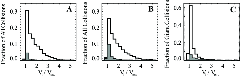
Figure 2.— Distribution of impact velocities normalized to mutual surface escape velocity for (A) all collisions (black line) and all giant impacts (filled grey) in group 1; (B) all collisions (black line) and all giant impacts (filled grey) in group 2; (C) all giant impacts (black line) and last giant impact (filled grey) in group 3 $N$-body simulations.

There were a total of 1207 collisions by planetesimals and embryos during the growth of the 15 planets in group 1. Of these, 1140 collisions were by planetesimals. The analytic model predicts that the majority of planetesimal collisions will lead to partial accretion (73%). The dominance of accretionary events is foremost a reflection of the impact velocity distribution, which is peaked between 1 and $2V_{\rm esc}$ (Figure 2A). Note that only half of the planetesimal is accreted onto an embryo when $V_{i}=2V_{\rm esc}$ (the critical velocity for accretion of half the projectile rises slightly with increasing impact angle, see Figure 1B). The distribution of accretion efficiencies ($(M_{\rm lr}-M_{\rm t})/M_{\rm p}$) from Asphaug, 2009) is shown in Figure 3A. The most common outcome of a planetesimal encounter was accretion of $>90$% of the mass, although there were a significant number of events where less material was accreted. For collisions between embryos, a smaller fraction of the projectile is accreted (70 to 90% for the 18 partial accretion events).

Beginning with Mars-sized embryos, there were no cases of erosion of the growing planet from planetesimal encounters. Notably, a substantial fraction of planetesimal encounters were hit-and-run events. For the initial 1:43 mass ratio between the planetesimals and embryos, the critical impact parameter is about 0.78 (51^∘). Given the probability distribution of impact angles, about 40% of outcomes for 1:43 mass ratio collisions are in the grazing regime, and the probability decreases as the embryos grow and the mass difference increases. Of all the impacts by planetesimals during the growth of Earth-mass planets, about 4% were graze-and-merge and 24% were hit-and-run. Erosion of the planetesimal occurred in nearly all of the hit-and-run collisions (253 out of 269), and catastrophic disruption of the planetesimal occured in about 85% of these events (Figure 1B).

Next, we consider only the giant impacts in group 1. Giant collision outcomes are approximately evenly split between partial accretion, graze-and-merge, and hit-and-run. Only a few of the embryo projectiles in hit-and-run events are eroded; in these collisions, the target and projectile have comparable masses ($\gamma\geq 0.1$) and neither body is disrupted.

The largest impact velocities ($>6V_{\rm esc}$), although rare, are high enough for embryos to catastrophically disrupt each other. There are notable examples of partial erosion (planet CJS1.4) and super-catastrophic (planet EJS1.4) outcomes. The last giant impact (at 222 Myr) onto a $1.05M_{\rm Earth}$ planet by a $0.1M_{\rm Earth}$ embryo at $3.2V_{\rm esc}$ and $35^{\circ}$ resulted in erosion of about 1% of the target mass (Figure 1A). The second giant impact (at 9.7 Myr) onto a $0.21M_{\rm Earth}$ body by a $0.147M_{\rm Earth}$ embryo at $6.2V_{\rm esc}$ and $26^{\circ}$ super-catastrophically disrupted the target leaving a largest remnant of only $0.008M_{\rm Earth}$.

3.1.2 Group 2

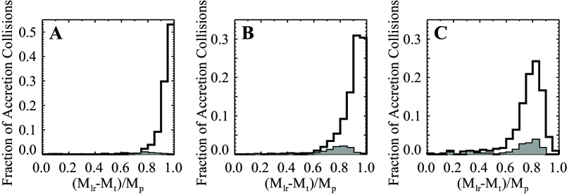
Figure 3.— Distribution of accretion efficiency ($(M_{\rm lr}-M_{\rm t})/M_{\rm p}$) for collisions that result in partial accretion: (A) all collisions (black line) and giant impacts (filled grey) in group 1; (B) all collisions (black line) and all giant impacts (filled grey) in group 2; (C) all giant impacts (black line) and last giant impact (filled grey) in group 3 $N$-body simulations.

There were a total of 3686 collisions by planetesimals and embryos during the growth of the 52 planets in group 2. Of these, 3142 collisions were by planetesimals. As in group 1, the analytic model predicts that about 70% of planetesimal collisions will lead to partial accretion. The simulations by Raymond et al. (2009) considered a wider range of dynamical configurations for Jupiter and Saturn, which produced a slightly wider distribution of impact velocities (Figure 2B) compared to group 1. In addition, the initial masses of the embryos was smaller. As a result, a couple of percent of planetesimals impacts led to erosion of the growing planet. For collisions in the partial accretion regime, the mean accretion efficiency is slightly lower in group 2 and the tail of low efficiency events is more pronounced than in group 1 (Figure 3B).

Overall, the probabilities of different collision outcomes for planetesimal impacts are similar in groups 1 and 2 because of the similar mass ratios and impact velocity distributions (Table 1). Again, most of the planetesimal hit-and-run events result in catastrophic disruption of the projectile.

Compared to the giant impacts in group 1, group 2 giant impacts have more partial accretion events and significantly more embryos are eroded in hit-and-run events. The difference is primarily a result of the fact that the initial embryos were smaller in the simulations by Raymond et al. (2009). The larger mass ratio between the embryos and growing planet leads to more cases of fragmentation of the smaller body and fewer grazing impacts. 22% of giant impacts in group 2 have $\gamma<0.1$, but only 4% of group 1 giant impacts have such a large mass contrast (Figure 4).

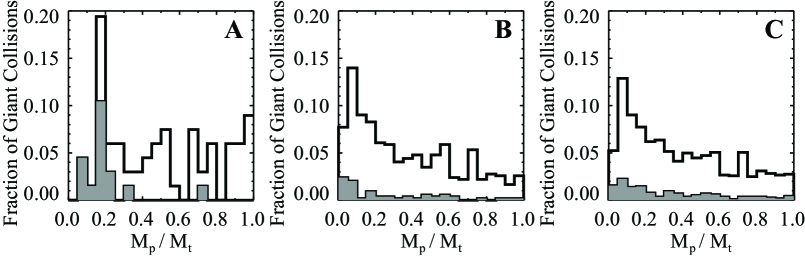
Figure 4.— Distribution of projectile-to-target mass ratio for all giant impacts (black lines) and last giant impact (filled grey) for (A) group 1; (B) group 2; (C) group 3 $N$-body simulations.

Of the 151 hit-and-run giant impacts in group 2, 75 projectiles were eroded (50%), and 29 projectiles suffered catastrophic disruption level fragmentation (19%). The three erosive giant impacts in this group removed 16, 6, and 1% of the material from target bodies with initial masses of 0.08, 0.50 and $0.72M_{\rm Earth}$, respectively. The erosive events all occurred in the eccentric Jupiter and Saturn (EJS) group of simulations with impact velocities between 2.1 and $3.2V_{\rm esc}$.

Because partial accretion is the most common outcome of non-grazing collisions, a significant fraction of giant impacts result in potentially observable changes in the bulk composition of a planet (Table 1). For collisions between differentiated bodies, the core-to-mantle mass ratio changes during both partial accretion and erosion events. For the large final planets in group 2, a 5% or greater increase in the mass fraction of the core, $f_{\rm core}$, occured in about 41% of all giant impacts and in about 20% of last giant impacts.

3.1.3 Group 3

Considering all 1165 giant impacts onto 161 planets in 40 planet formation simulations, the outcomes are approximately evenly split between partial accretion, graze-and-merge, and hit-and-run. Erosive events, including super-catastrophic disruption, occur about 1% of the time. In the hit-and-run events, about half of the projectiles are eroded and about 20% are catastrophically disrupted.

The equal likelihood of partial accretion, graze-and-merge, and hit-and-run is a result of the range of mass ratios and impact velocities for giant impacts. Given the impact velocity distribution in group 3, the velocity axis of a collision outcome map may be scaled by probability. In Figure 5, both axes are scaled by probability; hence, the area of each collision outcome (denoted by colors) is directly proportional to their probability.

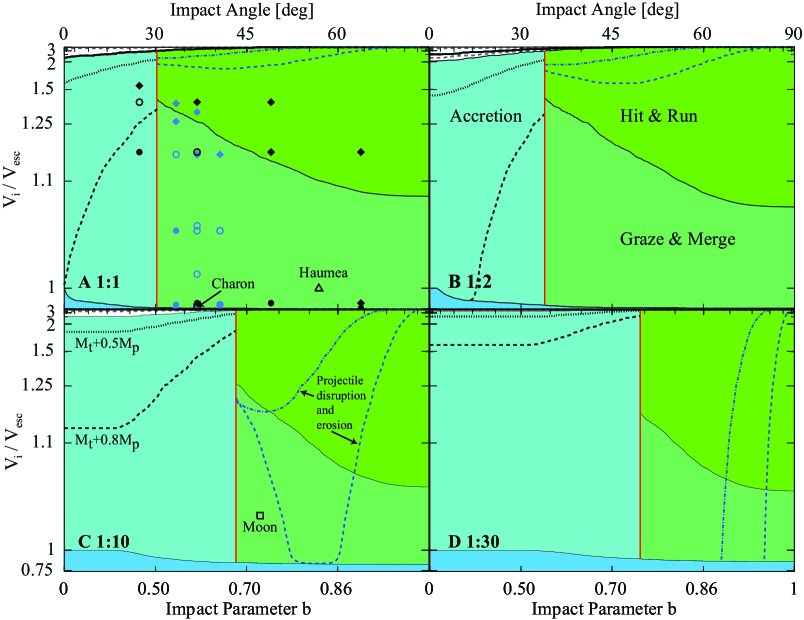
Figure 5.— Collision outcome maps with area scaled by outcome probability. Collision maps for planetary embryos, using material parameters $c^{*}=1.9$, $\bar{\mu}=0.36$, for projectile-to-target mass ratios of (A) $M_{\rm p}:M_{\rm t}=1:1$, (B) 1:2, (C) 1:10, and (D) 1:30. Vertical axis is scaled by velocity distribution of giant impacts in group 3 $N$-body simulations (Figure 2). Colors are the same as in Figure 1. Dotted black curve – 50% of projectile accreted; dashed black curve – 80% of projectile accreted; dot-dashed blue curve – catastrophic disruption of projectile in a hit-and-run; dashed blue curve – onset of erosion of projectile in a hit-and-run. Example results from numerical simulations: filled circles are merging, open circles and graze-and-merge, diamons are hit-and-run. Black – planetesimal collisions from Leinhardt et al. (2000); blue – Haumea formation simulations and favored Haumea impact scenario (triangle) from Leinhardt et al. (2010); arrow – disk-origin scenario for Charon from Canup (2005); square – typical moon formation scenario from Canup (2004).

The 4 panels span the range of giant impact mass ratios in group 3 (99% of events have $\gamma>0.03$ but a few embryo-embryo collisions have mass ratios as extreme as 1:55). Note that, over the course of the entire simulation, the mass ratio of a giant impact is about equally likely to fall anywhere between 0.03 and 1 (Figure 4C). Even when considering just the largest final planets (group 2), giant impacts may be any mass ratio (e.g., a collision between two $0.4M_{\rm Earth}$ bodies). However, the last giant impact onto target bodies greater than about $0.8M_{\rm Earth}$ are dominated by mass ratios less than 0.1 (Figure A.2F).

The collision maps fully scaled by probability emphasize the importance of the graze-and-merge regime even though it is a narrow regime in absolute impact velocity. The scaled figures also emphasize that partial accretion of the projectile is the most common outcome for non-grazing collisions; recall that the accretion efficiency peaks at about 80% for all giant impacts (Figure 3C). As shown in Figure 5, hit-and-run events occur about 1/3 of the time and the projectile is eroded when the projectile mass is less than about 10% of the target.

Note that the boundary between graze-and-merge and the adjacent partial accretion and hit-and-run regimes derived by Kokubo & Genda (2010) is generally in good agreement with other simulations with $\gamma=1$. However, the simulations of rubble pile collisions with $\gamma=0.5$ using the pkdgrav code (Leinhardt et al., 2010) found a much narrower graze-and-merge regime compared to the boundary derived from SPH simulations of fluid bodies. More work is needed to understand the boundaries of the graze-and-merge regime and its dependence on material properties.

As shown in Table 1, the last giant impact was more likely to be erosive (5%) or to be a hit-and-run (37%) compared to all giant impacts. The dynamical stirring by the last remaining planets leads to higher impact velocities near the end of planet formation compared to the total time average. In Figure 2C, note that the distribution of impact velocites is more weighted to values $>1.25V_{\rm esc}$ for the last impact (grey filled histogram) compared to all giant impacts (black histogram). For the same reason, more of the projectiles in the last giant hit-and-run event are eroded compared to all giant impacts (35 out of 60 events).

3.2. Collisions between planetesimals

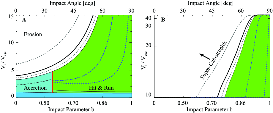
Figure 6.— Collision outcome maps for collisions between planetesimals with projectile-to-target mass ratio $M_{\rm p}:M_{\rm t}=1:2$ and material parameters of $c^{*}=5$ and $\bar{\mu}=0.37$, which are appropriate for a wide range of solid compositions. (A) Map with linear impact velocity normalized to planetesimal escape velocity and impact angle scaled by probability, and (B) map with area scaled to outcome probability for typical collision velocities stirred up by the presence of growing planets. Colors are the same as in Figure 1. Thick black curve – critical velocity for catastrophic disruption ($M_{\rm lr}=0.5M_{\rm tot}$); dashed grey curves – 10% and 90% of target mass in largest remnant; dotted black curve – 50% of projectile accreted; dot-dashed blue curve – catastrophic disruption of projectile in a hit-and-run; dashed blue curve – onset of erosion of projectile in a hit-and-run.

Note that the collisions considered in groups 1–3 are only those that contributed to the formation of the final planets. At the beginning of the simulation, there should have been many collisions between planetesimals, but they were not modeled. The collision outcome map for impacts between planetesimals with a mass ratio of 1:2 is shown in Figure 6. Typical planetesimal-planetesimal impact velocities will be similar to their collision velocities onto the embryos (about the escape velocity from the embryo, Figure 2). The surface escape velocity from an Earth-mass body is about 10 times the escape velocity from a $0.0025M_{\rm Earth}$ planetesimal. Erosion during collisions between comparable mass planetesimals begins at about $3.6V_{\rm esc}$ for $c^{*}=5$, a value appropriate for a variety of solid compositions. Hence, the most common planetesimal-planetesimal collision outcome is super-catastrophic destruction of the planetesimals. The probability-scaled collision map (Figure 6B) emphasizes the extremely destructive nature of planetesimal-planetesimal collisions in the presence of growing planets.

As shown in Figure 6B, collisions more oblique than about $60^{\circ}$ are hit-and-run. If planetesimal-planetesimal collisions had been modeled in the $N$-body simulations, the probability of a hit-and-run would have been artifically high at the beginning of the calculation because of the assumed starting distribution of equal-mass planetesimals. In fact, planetesimals in a size distribution defined by a collisional cascade would have a smaller fraction of mutual hit-and-run events. The ultimate fate of the smallest fragments in the collisional cascade is determined by the competition between accretion onto the growing planets and removal from the planet’s feeding zone (e.g., via Poynting-Robertson drag).

In the $N$-body simulations, the planetesimals all had the same mass because of computational limitations that restrict the total number particles. A tractable number of particles (few thousand) was insufficient to resolve a size distribution of planetesimals. However, the fraction of planetesimal collisions onto embryos that lead to partial accretion vs. hit-and-run depends on the mass ratio. If more of the mass in planetesimals were in smaller bodies, then accretionary collisions would be more common than found in the $N$-body simulations considered here.

4. A Monte Carlo Planet Growth Model

The restrospective analysis of $N$-body simulations presented above provides a limited view into the role of more realistic collision physics on planet growth because it cannot assess the cumulative effects of different collision outcomes. Studying suites of Monte Carlo simulations of the growth of a single planet via giant collisions allows for an intermediate examination of the role of collisions that is more tractable than many new full $N$-body simulations. The purpose of this Monte Carlo simulation is to investigate the effects of the collision physics model and is not meant to replace full $N$-body planet formation models or more sophisticated statistical population synthesis models (e.g., Alibert et al., 2011; Mordasini et al., 2009a, b; Ida & Lin, 2010).

4.1. Method

Our planet growth model assumed that the overall dynamics of giant impacts is similar to the $N$-body simulations by Raymond et al. (2009). Because planetary embryos become dynamically isolated when their masses are much smaller than an Earth-mass planet (roughly one tenth the mass), most of the mass in large terrestrial planets, here defined as a final mass $\geq 0.7M_{\rm Earth}$, is accreted via giant impacts (Kokubo & Ida, 1998). Thus, the Monte Carlo simulation uses the distribution of impact parameters from the group 3 $N$-body simulations to model planet growth (summarized in Figures A.1 and A.2). In the group 3 planets, the fraction of mass accreted via planetesimal collisions varied from 0 to 48%. The distribution of mass accreted from planetesimals is sensitive to the final mass of the planet; the large planets accreted between 2 and 27% of their final mass from planetesimals in the stochastic stage of planet formation modeled in the $N$-body simulations (Figure A.1).

For each planet, the following procedure was applied:

1. Randomly choose a value from the probability distribution of initial masses (Figure A.1). The minimum initial embryo mass was $0.01M_{\rm Earth}$.

2. Randomly choose a value from the probability distribution of number of giant impacts (Figure A.1).

3. For each giant impact, randomly choose the projectile mass, impact velocity, and impact angle. Projectile mass and impact velocity distributions are dependent on target mass (Figure A.2).

4. Three sets of simulations were run: (i) perfect merging for all collisions for comparison to the $N$-body results; (ii) collision physics assuming no re-impact by the projectile in hit-and-run events (group A); and (iii) collision physics assuming re-impact by the projectile in hit-and-run events (group B).

5. Add a randomly chosen value from the probability distribution of mass contributions from planetesimals. The planetesimal contribution distribution is also dependent on target mass (Figure A.1).

For each simulation set, we modeled the growth of 200 planets. When using the collision physics model, we tracked the core mass fraction assuming that all embryos have an initial value of 1/3 to be comparable to the bulk Earth. The core mass fraction of planetesimals was assumed to be the same as the initial embryos. We recorded the mass of debris produced by each giant impact. For the purpose of comparing perfect merging and the collision model, we assumed that all debris was lost and not reaccreted later. This end member assumption represents the maximum effect of fragmentation on inhibiting planet growth in the giant impact stage.

The distributions of impact velocities and projectile-to-target mass ratios are significantly dependent on the target mass (see Figure A.2). The population of initial embryos collides with each other to grow the first mid-size planets. The most common collision mass ratio depends on the initial size distribution of embryos assumed in a particular $N$-body simulation. During this early period of growth in the group 3 simulations, the mass ratios of the two bodies was about equally distributed between $0<\gamma<1$ (Figure A.2D). At the same time, the impact velocities are strongly peaked just above $1V_{\rm esc}$ (Figure A.2A) and few collisions lead to erosion (Figure A.2G). As the planets continue to grow, impacts onto the larger bodies are dominated by smaller embryos, and the distribution of mass ratios is strongly peaked with $\gamma<0.2$ for Earth-mass targets (Figure A.2F). The largest planets are strong perturbers on the remaining small embryos and the distribution of impact velocities becomes wider compared to earlier planet growth, spanning $1-3V_{\rm esc}$ (Figure A.2C).

If these mass-dependent effects were not included and the mean distributions were utilized instead, then the Monte Carlo model would predict too many very large planets ($>1.5M_{\rm Earth}$). In other words, the very end of terrestrial planet growth has distinct dynamical differences from earlier parts of the stochastic giant impact phase. To account for the variations with time, the values for impact velocity and mass ratio were chosen from the subset of group 3 collisions within $\pm 0.1M_{\rm Earth}$; when the target had a mass greater than one Earth mass, the distribution was based on the group 3 data with $M_{\rm t}>0.9M_{\rm Earth}$.

The projectile mass may be eroded during hit-and-run events. Therefore, in the group B set, we calculated the mass of the largest projectile remnant using the reverse collision scenario. The returning projectile had the mass of the largest remnant and the rest of the projectile debris was neglected. The re-impact had a randomly chosen impact angle and an impact velocity given by the greater of $V_{i}\sin\theta$ or $V_{\rm esc}$ after Kokubo & Genda (2010). The monotonically lowering re-impact velocity is an idealization that assumes that no interactions with other embryos led to an increase in the re-impact velocity. A projectile may hit-and-run several times before finally accreting or being disrupted. The hit-and-run sequence ended when the collision outcome was partial erosion, partial accretion, merging, or graze-and-merge. If the hit-and-run sequence eroded the projectile to less than one third of its original mass, it was assumed to be debris and neglected. As material was stripped from the escaping projectile, it was assumed to be derived from the projectile’s mantle, which raised its core mass fraction. In this way, the core mass fraction of a planet may be enriched after a sequence of hit-and-run events followed by a merging event.

4.2. Results

Table 2 Monte Carlo planet growth simulation results for 200 planets using the collision physics model and assuming (group A) no re-impact by a hit-and-run projectile and (group B) with re-impact. Assuming perfect merging only, 1455 giant impacts grew 200 planets with final masses up to $2.0M_{\rm Earth}$. Of these, 50 planets with masses $\geq 0.7M_{\rm Earth}$ grew from 651 giant impacts. For comparison, in the group 3 $N$-body simulations, 52 of 161 planets had final masses $\geq 0.7M_{\rm Earth}$. Collision material parameters were $c^{*}=1.9$ and $\bar{\mu}=0.36$ for hydrodynamic planets.

	Group A				Group B
	No hit-and-run return				With hit-and-run return
	15 Planets $0.7-1.31M_{\rm Earth}$				34 Planets $0.7-1.61M_{\rm Earth}$
	200 Planets		$\geq 0.7M_{\rm Earth}$		200 Planets		$\geq 0.7M_{\rm Earth}$
Collision outcome	$N=1455$	%	$N=190$	%	$N=1805$	%	$N=570$	%
Super-catastrophic	3	$<1$	0	0	5	$<1$	0	0
Partial erosion	9	$<1$	1	$<1$	17	$<1$	6	1
Partial accretion	489	34	70	37	619	34	194	34
Perfect merging	106	7	17	9	103	6	31	5
Graze-and-merge	571	39	56	29	671	37	166	29
Hit-and-run (H&R)	277	19	31	16	390	22	139	24
Special cases
H&R with proj. erosion	110	8	14	7	185	10	76	13
$5-10$% increase in final $f_{\rm core}$	43/200	22	4/15	27	45/200	23	9/34	26
$>10$% increase in final $f_{\rm core}$	53/200	27	9/15	60	71/200	36	19/34	56

Figure 7.— Monte Carlo planet growth simulation results. Mass distributions, core mass fractions, and debris mass (grey filled histograms) for 200 planet growth calculations assuming (A) perfect merging, (B,D,F) collision physics model with no hit-and-run return collisions, and (C,E,G) collision physics model with re-impact by hit-and-run projectile. Black line histogram in A-C is mass distribution of planets from group 3 $N$-body simulations. Black filled histograms in D-G are for planets with final masses $\geq 0.7M_{\rm Earth}$.

The distribution of final planet masses was calculated for each simulation set. The random number seed was the same for each group, so the differences are entirely a results of the collision model assumptions. The Monte Carlo simulations results are summarized in Table 2 and Figure 7. Details of the simulation parameters in each set is given in appendix figures A.3, A.4, and A.5. Here, we focus on the properties of the largest planets with final masses $>0.7M_{\rm Earth}$. The time between giant impacts was not considered here because the collision physics model may change the time scale for planet growth (see § 5).

In Figure 7, the mass distribution of final planets in the perfect merging simulation is similar to the group 3 $N$-body results, although the Monte Carlo model does not produce the same number of mid-size planets. The distribution of final planet masses is significantly smaller when the collision physics model is included and hit-and-run returns are neglected (group A). In the group 3 set of $N$-body simulations, 52 of the 161 planets (32%) had final masses $>0.7M_{\rm Earth}$. In the perfect merging Monte Carlo simulation, 50 of 200 planets (25%) reach final masses $>0.7M_{\rm Earth}$; however, in group A, the number of large planets drops to only 15 (7.5%). When hit-and-run return impacts are considered (group B), the final mass distribution of planets is between perfect merging and group A. In this case, 34 large planets are produced (17%).

During collisional growth and fragmentation, material is preferentially lost from the silicate mantle, thus raising the core mass fraction (Figure 7D,E). In simulation groups A and B, the maximum core mass fractions are 0.87 and 0.96, respectively, in bodies that experienced catastrophic impact events. Such core-dominated bodies are rare, and most (90-95%) final core mass fractions fall in the range of 0.33 to 0.4. In other words, most of the iron enrichment is within 20% of the initial value of $f_{\rm core}$. However, as a group, the largest planets are more likely to be enriched in core mass fraction compared to smaller planets. In both group A and B simulations, about 2/3 of the largest planets have core mass fractions greater than 10% of the initial value, compared to about 1/3 of all planets (Table 2). The largest planets experience a larger number of collisions which results in more cumulative erosion of the mantle.

The mass of debris produced during planetary growth by giant impacts can be significant. While there were planets that suffered only merging collisions that produced negligible debris (34 planets in group A and 25 in group B), they all had final masses of less than $0.38M_{\rm Earth}$ and an average of only 2 giant impacts. For comparison, the mean number of giant impacts was 7 and 9 for all planets in groups A and B, respectively. During the growth of large planets, debris production averaged 11% of the final planet mass in group A and 15% in group B (Figure 7F,G). The mass of debris reported in Figure 7 only includes debris from giant impacts; planetesimal collisions would also have contributed to the debris during planet growth.

In group A, the growth sequence that produced the most debris ($0.28M_{\rm Earth}$) suffered a penultimate erosive giant impact on a planet with final mass of only $0.22M_{\rm Earth}$. The most debris produced from one of the largest planets was 18% of a $1.31M_{\rm Earth}$ planet. Notably, there is a case of a $1.2M_{\rm Earth}$ planet in group B that produced $0.83M_{\rm Earth}$ of debris during its growth. In some cases, the growth sequence includes a step where the largest remnant is smaller than the initial embryo. Such destructive sequences occured for 4 planets in group A and 7 planets in group B.

An average of 12 giant impacts grew the largest planets in group A. With the inclusion of hit-and-run return events, an average of 16 giant impacts grew the largest planets in group B. In group B, the largest number of giant impacts for any planets was 26 (an ultimately $0.89M_{\rm Earth}$ planet), in contrast to the maximum of 18 giant impacts in group A. Hit-and-run return collisions often led to multiple re-impact events before the final merging or disruption of the projectile. The number of excess giant impacts in group B is shown in Figure 8. The mean number of extra collisions on the largest planets was 4 and ranged from 0 to 8.

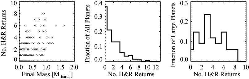
Figure 8.— Number of return hit-and-run (H&R) events in the group B Monte Carlo planet growth calculations. (A) Number of hit-and-run returns vs. final planet mass. Histogram of number of return events for (B) all 200 planets and (C) 34 planets with final masses $\geq 0.7M_{\rm Earth}$.

5. Discussion

This work demonstrates that the final, stochastic stage of terrestrial planet formation encompasses a diversity of collision outcomes. All types of collisions, from super-catastrophic disruption to perfect merging, are possible. Previous work that assumed perfect merging for all collisions were not capturing the full complexity of the giant impact phase. For the expected dynamical conditions for the terrestrial planets in our early Solar System, the principal collisions outcomes are approximately evenly split between partial accretion, hit-and-run, and graze-and-merge.

Because the collision outcome depends on mass ratio, the initial growth of planets via giant impacts is sensitive to the assumed mass distribution of planetary embryos. Because different numerical methods are typically used to model the growth of embryos (the oligarchic phase) and the end stage of planet formation (the stochastic phase), the discontinuity in technique has led to significant variation in the assumed initial number of embryos spread over different radial distances in different $N$-body studies. For example, Raymond et al. (2009) began with 85 to 90 embryos between 0.5 and 4.5 AU and O’Brien et al. (2006) assumed 25 embryos between 0.3 and 4 AU. Both included a population of equal-sized planetesimals. In contrast, Kokubo et al. (2006) began with 5 to 30 embryos between 0.5 and 1.5 AU and no planetesimals, and Kokubo & Genda (2010) assumed 16 initial embryos with no planetesimals over the same distance from the Sun.

In all $N$-body simulations, the initial masses and radial distributions of embryos are motivated by the isolation mass achieved at the end of oligarchic growth (e.g., Kokubo & Ida, 1998). However, the time scale to reach isolation is a function of radial distance and surface density, whereas the initial state of $N$-body simulations implies that the isolation masses have been reached everywhere at the same time. As a result, the number and size distributions of embryos and planetesimals are not perfectly linked to earlier stages of planet formation.

To address this problem, a few groups have recently developed hybrid computational techniques that may link more seamlessly the oligarchic growth and the stochastic end stage of planet formation (Levison et al., 2005; Bromley & Kenyon, 2006, 2011; Morishima et al., 2010). The current suite of hybrid techniques are based on very different approaches with different strengths and weaknesses. In this work, we have demonstrated that the end stage of planet formation involves significant fragmentation. Because the number of gravitationally interacting particles is limited in direct $N$-body techniques, hybrid methods that may include large numbers of smaller bodies (dust to planetesimals) are required to be able to fully model the giant impact stage.

5.1. Fragmentation during the giant impact stage

Fragmentation is a significant component of the giant impact stage of terrestrial planet formation. Fragmentation occurs primarily during partial accretion events and in erosion of the projectile in hit-and-run events. About 1/3 of giant impacts lead to partial accretion and about 1/3 are hit-and-run events. Of the hit-and-run events, about half are energetic enough to erode the projectile (Table 2). A small amount of escaping debris is created in some graze-and-merge events; however, the amount has not been quantified in our simulations as it is comparable to the resolution limit (of order 1% of the mass) (Leinhardt & Stewart, 2012). In Figure 5, the contours for projectile erosion (blue dashed line) extend into the graze-and-merge regime for collisions with a mass ratio more extreme than 1:7. Overall, about half of all giant impacts create significant (greater than about 1% of the total mass) debris.

In contrast, events that lead to erosion of the larger body are rare. All types of target erosion events (partial erosion to super-catastrophic disruption) occur about 1% of the time. Although infrequent, the conditions required to strip Mercury’s mantle by a single giant impact are included in the range of collision outcomes in the early Solar System.

To date, numerical simulations that include full fragmentation models have focused on earlier stages of planet formation, from dust to planetesimals to oligarchs (e.g., Kenyon & Luu, 1999; Bromley & Kenyon, 2011; Leinhardt & Richardson, 2005; Leinhardt et al., 2009; Chambers, 2008; Kobayashi et al., 2010). In these studies, fragmentation laws were defined by a size-dependent catastrophic disruption criteria such as derived by Benz & Asphaug (1999) (similar to equation 2 but including a strength regime for bodies smaller than about 1 km in radius). The previous fragmentation models have assumed that the disruption criteria follows pure energy scaling. Under pure energy scaling, the magnitude of the impact velocity does not influence the threshold energy for disruption (and $\bar{\mu}=2/3$ in equation 2). In other words, the disruption criteria for a particular size target only depended on the specific energy of the impact $M_{\rm p}V^{2}_{i}/M_{\rm t}$. In Stewart & Leinhardt (2009) and Leinhardt & Stewart (2012), we showed that this assumption is invalid.

In fact, catastrophic disruption follows nearly pure momentum scaling, where $\bar{\mu}=1/3$ (Leinhardt & Stewart, 2012). As a result, the disruption threshold is sensitive to the magnitude of the impact velocity by the factor $V^{*(2-3\bar{\mu})}$ in equation 2. Because most numerical and laboratory disruption experiments have involved projectiles that are much smaller than the target, most of the published disruption criteria are specifically for high impact velocities and extreme projectile-to-target mass ratios. Hence, when the collision involves two bodies that are more similar in mass, the applied disruption criteria are too high and the frequency of disruption is underestimated.

Stewart & Leinhardt (2009) compiled disruption data over a wide range of mass ratios in both the strength and gravity regimes to conclude that energy scaling was incorrect and the results were closer to momentum scaling. In Leinhardt & Stewart (2012), we derived a general analytic model for the disruption criteria in the gravity regime and fit material parameters for a range of target body types from solid planetesimals to fluid planets. Future work will tackle catastrophic disruption in the strength regime.

Now, future models of planet formation have a robust analytic model for fragmentation during collisions between gravity-dominated bodies. Our estimate of the magnitude of debris production, on average 15% of the mass in the largest planets, is in excellent agreement with preliminary results from multi-scale $N$-body and hydrocode calculations. Genda et al. (2011) calculated the very end stage of planet formation, beginning with 16 embryos and a total mass of 2.3 $M_{\rm Earth}$, using an $N$-body code. For each collision, the outcome was calculated by an SPH hydrocode simulation. The largest remnant or the two hit-and-run bodies were re-inserted into the $N$-body calculation and the debris was neglected. The cumulative mass of the fragments was about 22% of the total mass ($0.48M_{\rm Earth}$). Such multi-scale calculations are extremely computationally expensive, and the analytic model will allow for more and more detailed investigations of planet formation.

The need to track many small fragments is a significant challenge in models of the end stage of planet formation. The dynamical interactions between the protoplanets must be calculated by direct $N$-body techniques, but the smaller fragments will need to be treated statistically. As a result, detailed models of the giant impact stage must adopt new methods, such as the hybrid codes mentioned above. Hybrid models are needed to be able to calculate what fraction of the debris is reaccreted onto the final planets and what fraction is removed (e.g., via Poynting-Robertson drag). For fragments ground down below about 1 km in size, new disruption criteria are still needed in the strength regime that fully account for material properties, impact angle, mass ratio, and impact velocity.

5.2. Time scale of planet formation

The influence of more realistic collision physics on the time scale of terrestrial planet formation is difficult to predict because of competing factors. On one hand, the growth rate of planets is slower when outcomes other than perfect merging are included. On the other hand, the debris produced by collisions can influence the overall dynamics of the embryos and planetesimals (e.g., via dynamical friction, which could lead to more lower velocity collisions and more frequent merging outcomes).

The time scale for the end stage of planet formation was investigated in a recent study that included two collision outcomes. Kokubo & Genda (2010) conducted $N$-body simulations with a collision model that allowed for either perfect merging or an ideal hit-and-run event using their empirical boundary presented in equation 15 (which they applied at all impact angles). In a hit-and-run collision, neither body lost mass (there was no fragmentation) but the relative velocities of the bodies decreased. In simulations that began with 16 equal-mass embryos between 0.5 and 1.5 AU, they found that about half of the collisions were hit-and-run events. After a hit-and-run encounter, the reduced relative velocities led to a high probability of merging on the subsequent encounter. As a result, the time scale for planet growth was essentially the same as in simulations with the same starting conditions that assumed perfect merging.

The magnitude of any changes to planet growth time scales from different collision outcomes is sensitive to the initial conditions in the simulation. The simulations by Kokubo & Genda (2010) began with few relatively large embryos ($0.15M_{\earth}$) and no planetesimals. With this initial distribution of embryos, all collisions were between comparable mass bodies ($M_{\rm p}/M_{\rm t}>0.1$), which are the most likely to be graze-and-merge or hit-and-run events (Figure 5). Since the hit-and-run bodies are likely to recollide on time scales comparable to the orbital period, the overall effect of hit-and-run events on this very end stage of planet growth was found to be negligible. If fragmentation were included or if the sizes of the bodies were more diverse (e.g., with the inclusion of planetesimals or smaller initial embryos), more realistic collision outcomes would have a larger effect on planet growth. As mentioned above, using the same initial conditions in their multi-scale calculations, Genda et al. (2011) found that fragmentation was a significant process.

Although fragmentation makes planet growth from an individual collision less efficient, other effects from the debris may lead to faster planet growth overall or faster stages of planet growth. For example, during oligarchic growth, Chambers (2008) found that fragmentation led to faster growth of embryos because smaller fragments are more easily captured. However, fragmentation also decreased the surface density of solids in the disk (which limits the embryo’s final mass) because fragments were lost more quickly by drag processes as they were ground down in size. During the giant impact stage, O’Brien et al. (2006) found that the strong dynamical friction from 1000 planetesimals led to overall faster planet growth compared to studies without any planetesimals. However, their study assumed perfect merging for all collision outcomes and non-interacting planetesimals. If dynamical friction becomes very large, a gap could form in the planetesimal disk around an embryo, which would effectively halt the growth of that embryo. Hence, the role of fragmentation on planet growth time scales is not independent of other processes acting at the same time. Ultimately, because fragmentation is a critical process that feeds back into the dynamics of planet growth, new simulations that include both embryos and a fully interacting population of small bodies are needed to investigate how more realistic collision outcomes affect formation time scales.

5.3. Composition and chemistry of planets

We found that the core-to-mantle mass fraction increases during the growth of planets via fragmentation during collisions between differentiated embryos. Loss of the silicate mantle primarily occurred during partial accretion and erosion of the projectile in hit-and-run events. From our group B Monte Carlo calculations, the mean increase in the core mass fraction was 15% for the 34 largest planets (Figure 7E, black histogram). The magnitude of the core fraction increase is potentially observable in the study of the chemical composition of planets and early Solar System materials.

O’Neill & Palme (2008) argue that the Earth’s bulk iron to magnesium (Fe/Mg) ratio is significantly larger than the solar ratio. They propose that the Earth lost a portion of its silicate mantle during the giant impact stage, which raised the Fe/Mg ratio of the final planet compared to the more primitive (closer to nebular composition) materials that formed the planetary embryos. O’Neill & Palme (2008) estimate that the whole-Earth Fe/Mg mass ratio is $2.1\pm 0.1$. The Fe/Mg value for primitive materials is not known precisely. The solar photosphere value, $1.87\pm 0.4$ (Asplund et al., 2005), is too poorly constrained to be useful for such detailed comparisons. The Fe/Mg ratio for the solar wind will be constrained by Genesis mission. Early results suggested a lower value than the solar photosphere ($1.61\pm 0.23$, Jurewicz et al., 2011); however, final data calibration is still in progress (A. Jurewicz, pers. comm.). The Fe/Mg ratio for carbonaceous chondrites, the most primitive type of meteorite, is $1.92\pm 0.08$ (Palme & Jones, 2005). The available data suggest that the Earth is enriched in Fe/Mg compared to solar composition by approximately 10%.

Our Monte Carlo calculations of the cumulative effects of realistic collision outcomes are in excellent agreement with the collisional erosion idea proposed by O’Neill & Palme (2008). Although our planet growth models are not detailed enough to track individual elements, we use the core-to-mantle mass ratio as a proxy for the Fe/Mg ratio. About half of the largest planets in the group B calculations have core mass fraction enrichments of 10-30%. The mean is likely to be slightly lower than this range because some of the mantle fragments will be reaccreted. Assuming that the reaccretion process is less than 100% efficient, the largest terrestrial planets have a larger core mass fraction compared to the initial embryo composition as a result of fragmentation during giant impacts.

Bulk elemental ratios are difficult to derive for a planet, and more detailed information can be derived from examination of isotopic systems. The hafnium-tungsten (Hf-W) system, with a half life of 9 Myr, is a major constraint on the timing of planet formation. Both elements are refractory (high condensation temperatures); Hf is lithophile and is retained in the silicate mantle, while W is moderately siderophile and prefers the iron core. With assumptions about the extent of chemical equilibration between the metals and silicates within the growing planet, measurements of the present-day ratios of Hf and W isotopes constrain the time scale for planet formation, including the timing of the proposed Moon-forming impact (Jacobsen, 2005; Kleine et al., 2009).

Using 15 planets from the $N$-body simulations by O’Brien et al. (2006) (Group 1 in Table 1), Nimmo et al. (2010) calculated the evolution of the Hf-W system during planet growth in the giant impact stage and compared the results to observed values for Earth, the Moon, and Mars. The study varied the equilibration factor between two idealized end members: no equilibration, where the core from the projectile merges with the target core without any equilibration with the mantle, to perfect equilibration, where the projectile core completely equilibrates with the mantle. The equilibration factor was held constant during the entire growth of a planet; in reality, the extent of equilibration depends on the physics of material mixing during giant impacts, which is still rather poorly understood (e.g., Dahl & Stevenson, 2010). Nimmo et al. (2010) found that Earth-like Hf-W ratios could be generated if the iron cores partially equilibrated with the mantle; however, they could not simultaneously match both the Earth and the Moon. They suggest that either that the Earth and Moon equilibrated after the giant impact (Pahlevan & Stevenson, 2007) or that the time scales for planet growth are too short in the $N$-body simulations.

With more realistic collision physics in planet formation simulations, calculations of the evolution of the Hf-W system will be more robust. In particular, the collision model estimates the fraction of core and mantle incorporated during partial accretion of the projectile and following hit-and-run events with projectile erosion. Improving the time scale for planet growth, as discussed above, is essential for interpretation of the Hf-W system. Finally, improved physical models for mixing of metals and silicates during giant impacts are still needed.

Fragmentation during planet formation may also affect the final volatile content. Several studies have investigated possible sources of water in the Earth by assuming that the water content in condensed material varies monotonically with distance from the Sun. The initial locations of material that accretes into terrestrial planets have been used to investigate the formation of Earth-like planets under the assumption of perfect merging (e.g., Morbidelli et al., 2000; Raymond et al., 2004, 2007). The accretion of water to the Earth may now be investigated in greater detail.

The incorporation of volatiles in planets not only depends on the source location of the incoming material but also the specific collision scenario. Asphaug (2010) proposed that the volatile content of planetary bodies may be affected by hit-and-run events. Because erosion of the projectile is common in hit-and-run events, the projectile may be stripped of volatile-rich outer layers (including an atmosphere). If the hit-and-run projectile is later incorporated into a growing planet, the planet would be depleted in both volatiles and mantle material compared to the initial embryos.

The process of compositional changes via fragmentation is not restricted to the inner Solar System. The dwarf planets in the outer Solar System have higher bulk densities than smaller Kuiper Belt objects (Brown, 2008; Fraser & Brown, 2010). The bulk densities of dwarf planets may have increased during collisional growth by preferential stripping of the icy mantles from projectiles, possibly by partial accretion of planetesimals during runaway growth in addition to the limited number of giant impacts experienced by dwarf planets.

5.4. The graze-and-merge regime

The boundary between the graze-and-merge and hit-and-run regimes is not precisely known. In this work, we used the boundary defined from a single set of calculations for differentiated iron-silicate planets (Kokubo & Genda, 2010; Genda et al., 2012). The boundary is slightly different in the few other studies that have focused on this regime. In Figure 5, the results from different studies are plotted as symbols for comparison to the Kokubo & Genda (2010) graze-and-merge boundary.

Leinhardt et al. (2000) calculated the outcome of collisions between equal-mass rubble piles (black symbols). The collision velocities were subsonic between the 1-km radius bodies, so the study utilized the pkdgrav $N$-body code rather than a shock hydrocode. The results show that grazing outcomes extend to impact parameters slightly below $b_{\rm crit}$. For impact angles between about 30 and 50 degrees, the transition to hit-and-run is in good agreement with (Kokubo & Genda, 2010). However, at higher impact angles ($64^{\circ}$), the rubble pile collisions transitioned to hit-and-run at much lower impact velocities. Using the same code, Leinhardt et al. (2010) modeled collisions onto $\sim 700$ km radius bodies with equal mass and half mass projectiles (blue symbols in Figure 5A and B). The results for equal mass bodies support the same boundary as (Kokubo & Genda, 2010) for the 30 to $40^{\circ}$ impacts. However, the simulations for a mass ratio of 1:2 show a much faster transition to hit-and-run at an impact angle of $53^{\circ}$.

The different boundaries between graze-and-merge and hit-and-run may be primarily attributed to the relatively low resolution for all three studies. The studies were focused on other aspects of collisions and not to designed to resolve the interaction of very thin layers of material at high impact angles. In addition, small differences in dissipation of energy and momentum are likely to influence the transition to hit-and-run at high impact angles. If the graze-and-merge regime is smaller than considered here, the collisions would increase the fraction of hit-and-run events.

The graze-and-merge regime is believed to have left a strong mark in our Solar System. The formation of Earth’s Moon (Canup, 2004), the Pluto system (Canup, 2005), and the Haumea system (Leinhardt et al., 2010) are all attributed to graze-and-merge regime events (Figure 5). More work is needed to understand the details of moon formation in the graze-and-merge regime and the factors that control the transition between the graze-and-merge and hit-and-run regimes.

6. Conclusions

Using a new analytic collision physics model (Leinhardt & Stewart, 2012), we have investigated the range of collision outcomes during the stochastic end stage of planet formation. For the dynamical conditions expected in our early Solar System, the outcome of giant impacts span all possible regimes: hit-and-run, merging, partial accretion, partial erosion, and catastrophic disruption. Fragmentation during giant impacts is significant. During the formation of planets larger than $0.7M_{\rm Earth}$, the total mass of debris is about 15% of the final planet mass. Fragmentation occurs primarily by erosion of the smaller body in partial accretion and hit-and-run events. Future simulations of the end stage of planet formation will need to utilize hybrid techniques that are able to track both massive planets and a large population of smaller bodies. Assuming that fragments are not completely reaccreted, growth via giant impacts creates final planets are that depleted in volatiles and mantle material compared to the initial planetary embryos.

Acknowledgements. We thank D. O’Brien and S. Raymond for the $N$-body simulation data and valuable discussions. STS is supported by NASA grant # NNX09AP27G, ZML by a STFC Advanced Fellowship.

APPENDIX FIGURES

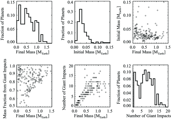
Figure A.1.— Distribution of parameters from group 3 $N$-body simulations. Distributions for initial mass, number of giant impacts, and mass contribution from planetesimals used in Monte Carlo planet growth simulations.

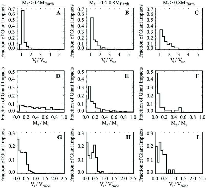
Figure A.2.— Distribution of impact velocities (A-C), projectile-to-target mass ratios (D-F), and ratio of impact velocity to velocity needed for onset of target erosion ($V_{\rm erode}$) (G-I) for all giant impacts in group 3 for $M_{\rm t}<0.4M_{\rm Earth}$ (left column), $0.4M_{\rm Earth}<M_{\rm t}<0.8M_{\rm Earth}$ (middle column), and $M_{\rm t}>0.8M_{\rm Earth}$ (right column). Target mass-dependent values for impact velocity and projectile-to-target mass ratios used in Monte Carlo planet growth simulations.

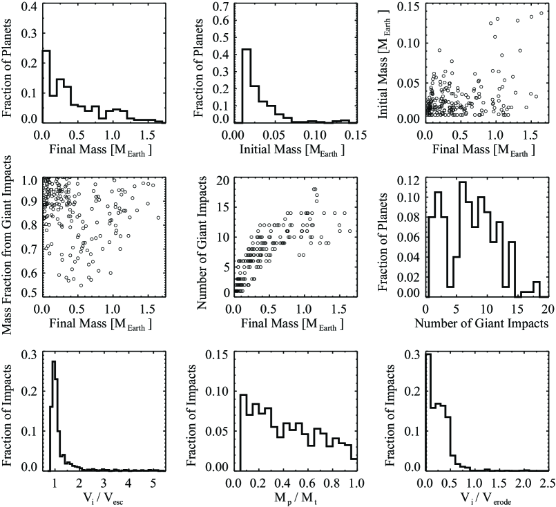
Figure A.3.— Distribution of parameters for 200 Monte Carlo planet growth simulations with perfect merging.

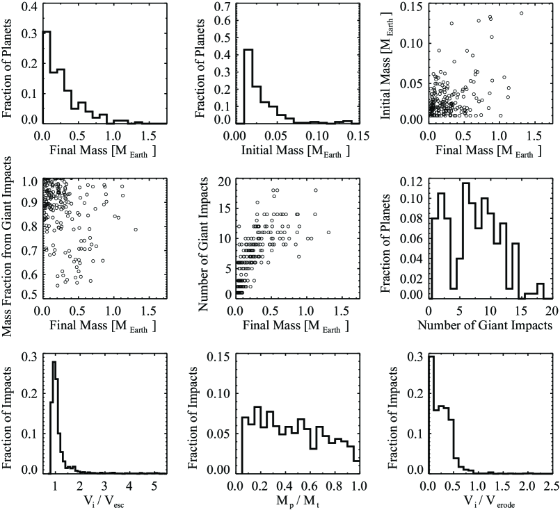
Figure A.4.— Distribution of parameters for 200 Monte Carlo planet growth simulations with collision physics model and assuming no re-impact by a hit-and-run projectile (group A).

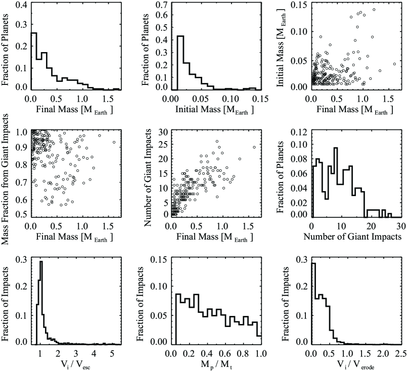
Figure A.5.— Distribution of parameters for 200 Monte Carlo planet growth simulation with collision physics model with re-impact by a hit-and-run projectile (group B). Note the increase in number of giant impacts compared to group A.

References

- Agnor & Asphaug (2004) Agnor, C., & Asphaug, E. 2004, ApJL, 613, L157
- Agnor et al. (1999) Agnor, C. B., Canup, R. M., & Levison, H. F. 1999, Icarus, 142, 219
- Alibert et al. (2011) Alibert, Y., Mordasini, C., & Benz, W. 2011, A&A, 526, A63
- Asphaug (2009) Asphaug, E. 2009, Ann. Rev. Earth Planet Sci., 37, 413
- Asphaug (2010) —. 2010, Chemie der Erde, 70, 199
- Asphaug et al. (2006) Asphaug, E., Agnor, C. B., & Williams, Q. 2006, Nature, 439, 155
- Asplund et al. (2005) Asplund, M., Grevesse, N., & Sauval, A. J. 2005, in ASP Conf. Series, Vol. 336, Cosmic Abundances as Records of Stellar Evolution and Nucleosynthesis, ed. T. G. Barnes III & F. N. Bash, 25–38
- Benz et al. (2007) Benz, W., Anic, A., Horner, J., & Whitby, J. A. 2007, Space Sci. Rev., 132, 189
- Benz & Asphaug (1999) Benz, W., & Asphaug, E. 1999, Icarus, 142, 5
- Bromley & Kenyon (2006) Bromley, B. C., & Kenyon, S. J. 2006, AJ, 131, 2737
- Bromley & Kenyon (2011) —. 2011, ApJ, 731, 101
- Brown (2008) Brown, M. E. 2008, The Solar System Beyond Neptune (U. Arizona Press), 335–344
- Canup (2004) Canup, R. M. 2004, Icarus, 168, 433
- Canup (2005) —. 2005, Science, 307, 546
- Canup & Asphaug (2001) Canup, R. M., & Asphaug, E. 2001, Nature, 412, 708
- Chambers (2008) Chambers, J. 2008, Icarus, 198, 256
- Chambers (1999) Chambers, J. E. 1999, MNRAS, 304, 793
- Chambers (2004) Chambers, J. E. 2004, Earth Planet. Sci. Lett., 223, 241
- Dahl & Stevenson (2010) Dahl, T. W., & Stevenson, D. J. 2010, Earth Planet. Sci. Lett., 295, 177
- Duncan et al. (1998) Duncan, M. J., Levison, H. F., & Lee, M. H. 1998, ApJ, 116, 2067
- Fraser & Brown (2010) Fraser, W. C., & Brown, M. E. 2010, ApJ, 714, 1547
- Genda et al. (2011) Genda, H., Kokubo, E., & Ida, S. 2011, Lunar Planet. Sci. Conf., 42, 2090
- Genda et al. (2012) —. 2012, ApJ, 744, 137
- Goldreich et al. (2004) Goldreich, P., Lithwick, Y., & Sari, R. 2004, ApJ, 614, 497
- Housen & Holsapple (1990) Housen, K. R., & Holsapple, K. A. 1990, Icarus, 84, 226
- Ida & Lin (2010) Ida, S., & Lin, D. N. C. 2010, ApJ, 719, 810
- Jacobsen (2005) Jacobsen, S. B. 2005, Ann. Rev. Earth Planet Sci., 33, 531
- Jurewicz et al. (2011) Jurewicz, A. J. G., Burnett, D. S., Woolum, D. S., McKeegan, K. D., Heber, V., Guan, Y., Humayun, M., & Hervig, R. 2011, Lunar Planet. Sci. Conf., 42, 1917
- Kenyon & Luu (1999) Kenyon, S. J., & Luu, J. X. 1999, AJ, 118, 1101
- Kleine et al. (2009) Kleine, T., Touboul, M., Bourdon, B., Nimmo, F., Mezger, K., Palme, H., Jacobsen, S. B., Yin, Q.-Z., & Halliday, A. N. 2009, Geochim. Cosmochim. Acta, 73, 5150
- Kobayashi et al. (2010) Kobayashi, H., Tanaka, H., Krivov, A. V., & Inaba, S. 2010, Icarus, 209, 836
- Kokubo & Genda (2010) Kokubo, E., & Genda, H. 2010, ApJL, 714, L21
- Kokubo & Ida (1998) Kokubo, E., & Ida, S. 1998, Icarus, 131, 171
- Kokubo et al. (2006) Kokubo, E., Kominami, J., & Ida, S. 2006, ApJ, 642, 1131
- Leinhardt et al. (2010) Leinhardt, Z. M., Marcus, R. A., & Stewart, S. T. 2010, ApJ, 714, 1789
- Leinhardt & Richardson (2005) Leinhardt, Z. M., & Richardson, D. C. 2005, ApJ, 625, 427
- Leinhardt et al. (2009) Leinhardt, Z. M., Richardson, D. C., Lufkin, G., & Haseltine, J. 2009, MNRAS, 396, 718
- Leinhardt et al. (2000) Leinhardt, Z. M., Richardson, D. C., & Quinn, T. 2000, Icarus, 146, 133
- Leinhardt & Stewart (2012) Leinhardt, Z. M., & Stewart, S. T. 2012, ApJ, 745, 79
- Levison et al. (2005) Levison, H., Nesvorny, D., Agnor, C., & Morbidelli, A. 2005, BAAS, 37, 666
- Lissauer (1993) Lissauer, J. J. 1993, Ann. Rev. Astron. & Astrophys., 31, 129
- Marcus et al. (2010) Marcus, R. A., Sasselov, D., Stewart, S. T., & Hernquist, L. 2010, ApJL, 719, L45
- Marcus et al. (2009) Marcus, R. A., Stewart, S. T., Sasselov, D., & Hernquist, L. 2009, ApJL, 700, L118
- Melosh & Ryan (1997) Melosh, H. J., & Ryan, E. V. 1997, Icarus, 129, 562
- Morbidelli (2010) Morbidelli, A. 2010, Comptes Rendus Physique, 11, 651
- Morbidelli et al. (2000) Morbidelli, A., Chambers, J., Lunine, J. I., Petit, J. M., Robert, F., Valsecchi, G. B., & Cyr, K. E. 2000, Met. Planet. Sci., 35, 1309
- Mordasini et al. (2009a) Mordasini, C., Alibert, Y., & Benz, W. 2009a, A&A, 501, 1139
- Mordasini et al. (2009b) Mordasini, C., Alibert, Y., Benz, W., & Naef, D. 2009b, A&A, 501, 1161
- Morishima et al. (2010) Morishima, R., Stadel, J., & Moore, B. 2010, Icarus, 207, 517
- Nimmo et al. (2010) Nimmo, F., O’Brien, D. P., & Kleine, T. 2010, Earth Planet. Sci. Lett., 292, 363
- O’Brien et al. (2006) O’Brien, D. P., Morbidelli, A., & Levison, H. F. 2006, Icarus, 184, 39
- O’Neill & Palme (2008) O’Neill, H. S., & Palme, H. 2008, Phil. Trans. R. Soc. Lond. A., 28, 4205
- Pahlevan & Stevenson (2007) Pahlevan, K., & Stevenson, D. J. 2007, Earth Planet. Sci. Lett., 262, 438
- Palme & Jones (2005) Palme, H., & Jones, A. 2005, Meteorites, Comets and Planets: Treatise on Geochemistry, Vol. 1 (Elsevier), 41–61
- Raymond et al. (2009) Raymond, S. N., O’Brien, D. P., Morbidelli, A., & Kaib, N. A. 2009, Icarus, 203, 644
- Raymond et al. (2004) Raymond, S. N., Quinn, T., & Lunine, J. I. 2004, Icarus, 168, 1
- Raymond et al. (2007) —. 2007, Astrobiology, 7, 66
- Shoemaker (1962) Shoemaker, E. M. 1962, Physics and Astronomy of the Moon (Academic Press), 283–359