Cosmokinetics: A joint analysis of Standard Candles, Rulers and Cosmic Clocks

Abstract

We study the accelerated expansion of the Universe by using the kinematic approach. In this context, we parameterize the deceleration parameter, $q(z)$, in a model independent way. Assuming three simple parameterizations we reconstruct $q(z)$. We do the joint analysis with combination of latest cosmological data consisting of standard candles (Supernovae Union2 sample), standard ruler (CMB/BAO), cosmic clocks (age of passively evolving galaxies) and Hubble ($H(z)$) data. Our results support the accelerated expansion of the Universe.

1 Introduction

Mapping the cosmic expansion history with accelerated expansion is one of the major challenges faced by modern cosmology. Various observations, directly (Type Ia Supernovae, SNe Ia) and indirectly (CMB, BAO, lookback time) provide evidence for the recently observed accelerated expansion of the Universe [1, 2, 3, 4, 5]. The phenomenon of acceleration is usually attributed to some sort of dark energy [6]. The effect of dark energy is to change the sign of ”deceleration parameter” $q(z)$. Whether estimates of $q(z)$ point towards accelerated or decelerated expansion, strongly depends on quality and quantity of the observational data at various redshifts. Therefore, one of the simple ways to understand the kinematics of the Universe is by phenomenologically parameterizing $q(z)$.

The phenomenological approach is advantageous since it does not rely on model specific assumptions like the composition of the Universe. It is assumed that our Universe is homogeneous and isotropic at large scales and is described by a metric theory of gravity. This type of approach is explained in literature in a variety of ways [7, 8, 9, 10, 11].

Following the same line of thought we reconstruct the deceleration parameter using the Supernovae Union2 data set, CMB/BAO, Hubble parameter data (H(z)), and lookback time (LBT). Since the nature of the driving force of the Universe is still a mystery, therefore the choice of parameterization of $q(z)$ is arbitrary. We use two two-parameter models of $q(z)$ and and one one-parameter model to reconstruct the deceleration parameter. Riess et al. [12] showed using Gold (SNe Ia) data set that $q(0)<0$ at $99\%$ confidence level, and there was a transition from recent acceleration to past deceleration. In this context the phenomenological approach to parameterize the $q(z)$ is an easy way to find out $q(0)$, and the transition redshift, $z_{t}$, where expansion switches from being decelerated to accelerated.

In addition to the data sets used in previous works, we have used the age of slowly evolving passive galaxies (lookback time) in our analysis. The addition of the LBT is significant as it is complementary to the observations used in previous works and may help us to obtain more realistic constraints on the expansion history.

The paper is organized as follows. In section II, we discuss the $q(z)$ parameterizations, data and methodology. The results and discussion are explained in section III.

2 Model, Data and Methodology

With the assumption that Universe is homogeneous and isotropic, and spatial flatness which is motivated by inflation and WMAP measurements [13], FRW metric describes the background geometry

$$ds^{2}=-dt^{2}+a(t)^{2}\left[dr^{2}+r^{2}d\Omega^{2}\right]\;.$$

Here $a(t)$ is the scale factor. The cosmic scale factor is related to the redshift of free streaming photons in the usual way: $a(t)=1/(1+z)$ . The expansion and deceleration rates can be defined as

$$H(z) \equiv \frac{\dot{a}}{a},$$ (2.1)

$$q(z) \equiv -\frac{a\ddot{a}}{{\dot{a}}^{2}}=\frac{d}{dt}H^{-1}-1\;,$$ (2.2)

where $H$ is the Hubble parameter. We can write the Hubble parameter as

$$H=H_{0}\exp{\left[\int^{z}_{0}\frac{1+q(z^{\prime})}{1+z^{\prime}}dz^{\prime}\right]}\;.$$ (2.3)

Here $H_{0}$ is the present value of the Hubble parameter.

We parameterize the redshift dependence of $q(z)$ in the following way,

$$q_{I}(z) =q_{0}+q_{1}z\;,$$

$$q_{II}(z) =q_{2}+q_{3}\frac{z}{1+z}\;,$$

$$q_{III}(z) =\frac{1}{2}+\frac{q_{4}}{(1+z)^{2}}\;.$$

The first parameterizations is a linear Taylor series expansion of the deceleration parameter around $z=0$, where $q_{0}$ and $q_{1}$ are its present value and its first derivative, respectively. The second parameterization has an advantage that it converges at high redshift, as expected. The last parameterization is such that it converges to the value $\frac{1}{2}$ at high redshift, which is the value of the deceleration parameter at matter dominated epoch.

In general the dark energy density parameter can be expressed as a function of redshift as

$$\Omega_{X}(z)=\Omega_{X0}\exp{\left[3\int^{z}_{0}\frac{1+w(z^{\prime})}{1+z^{\prime}}dz^{\prime}\right]}\,$$ (2.4)

where $w(z)$ is the equation of state and is related to $H(z)$ by

$$w(z)=\frac{\frac{2}{3}(1+z)\frac{dlnH}{dz}-1}{1-(\frac{H_{0}}{H})^{2}\ \Omega_{m0}(1+z)^{3}}.$$ (2.5)

Substituting for $H(z)$ we can express $w(z)$ in terms of the deceleration parameter q(z) as[14]

$$w(z)=\frac{\frac{2}{3}(1+q(z))-1}{1-\exp{\left[-2\int^{z}_{0}\frac{1+q(z^{\prime})}{1+z^{\prime}}dz^{\prime}\right]}\ \Omega_{m0}(1+z)^{3}}.$$ (2.6)

2.1 Lookback time

Most of the observations used for constraining cosmological parameters like SNe Ia, angular diameter distances etc. are distance based measurements. The LBT on the other hand is based on ages of distant galaxies.

The LBT to an object at redshift $z$ is defined as the difference between the present age of the Universe and its age at redshift $z$ and can be calculated as

$$t_{L}(z,p)=H_{0}^{-1}\int_{0}^{z}\frac{dz^{{}^{\prime}}}{(1+z^{{}^{\prime}}){\cal H}(p)}\;,$$ (2.7)

where ${\cal H}(p)$ is the dimensionless Hubble parameter ${\cal H}(p)\equiv H(p)/H_{0}$ and p are the parameters of the model. The observed lookback time $t_{L}^{obs}$ to an object at redshift $z_{i}$ is defined as

$$t_{L}^{obs}(z_{i},t_{inc},t_{0}^{obs})=t_{0}^{obs}-t(z_{i})-t_{inc}\;,$$ (2.8)

where $t_{0}^{obs}$ is the observed age of the Universe. $t(z_{i})$ is the age of the object defined as the difference between the age of the Universe at redshift $z_{i}$ and the age of the Universe when the object was born at redshift $z_{f}$.

$$t(z_{i},p)=H_{0}^{-1}\left[\int_{z_{i}}^{\infty}\frac{dz^{{}^{\prime}}}{(1+z^{{}^{\prime}}){\cal H}(p)}-\int_{z_{f}}^{\infty}\frac{dz^{{}^{\prime}}}{(1+z^{{}^{\prime}}){\cal H}(p)}\right]$$ (2.9)

or

$$t(z_{i},p)=H_{0}^{-1}\int_{z_{i}}^{z_{f}}\frac{dz^{{}^{\prime}}}{(1+z^{{}^{\prime}}){\cal H}(p)}$$ (2.10)

$t_{inc}=t_{0}^{obs}-t_{L}(z_{f})$ is the incubation time of the object. Since we don’t know the formation redshift of the objects in our sample, $t_{inc}$ is treated as a nuisance parameter and we marginalize over it.

From the definition of the LBT above, we can write

$$t_{L}(z,p)=H_{0}^{-1}\int_{0}^{z}\frac{dz^{{}^{\prime}}}{(1+z^{{}^{\prime}})\exp\left(\int^{z_{{}^{\prime}}}_{0}\frac{1+q(u)}{1+u}~{}du\right)}$$ (2.11)

Now, we can substitute for $q(z)$ and write the lookback time for the three different parameterization. In the first case we get

$$t_{L}(z,p)=H_{0}^{-1}\int_{0}^{z}(1+z^{{}^{\prime}})^{q_{1}-q_{0}-2}\exp(-q_{1}z^{{}^{\prime}})~{}dz^{{}^{\prime}}$$ (2.12)

For the second parameterization the lookback time can be written as

$$t_{L}(z,p)=H_{0}^{-1}q_{2}^{-q_{2}-q_{3}-1}\left[\gamma(q_{2}+q_{3}+1,q_{3})-\gamma\left(q_{2}+q_{3}+1,\frac{q_{3}}{1+z}\right)\right]$$ (2.13)

where $\gamma$ is the incomplete gamma function. For the last case, we get

$$t_{L}(z,p)=H_{0}^{-1}\exp\left(-\frac{q_{4}}{2}\right)\int_{0}^{z}\frac{\exp\left(\frac{q_{4}}{2(1+z^{{}^{\prime}})^{2}}\right)}{(1+z^{{}^{\prime}})^{5/2}}~{}dz^{{}^{\prime}}$$ (2.14)

To constrain the parameters we use the ages of 32 passively evolving galaxies in the redshift interval $0.117\leq z\leq 1.845$ [15]. We assume a 12$\%$ one standard deviation uncertainty on the age measurements. The value of the Hubble parameter $H_{0}$ is fixed at $H_{0}=$ 74.2 km/sec/Mpc and the age of the Universe is taken to be $t_{0}^{obs}=$ 13.75 $\pm$ 0.13 Gyr.

The likelihood function is defined as

$${\cal L}\propto\exp\left(-\frac{\chi^{2}}{2}\right)$$ (2.15)

where $\chi^{2}$ is given by

$$\chi^{2}(p,H_{0},t_{inc},t_{obs})=\sum_{i=1}^{32}\frac{(t_{L}(z_{i},p,H_{0})-t_{L}^{obs}(z_{i},t_{inc},t_{0}^{obs}))^{2}}{\sigma_{i}^{2}+\sigma_{t_{0}^{obs}}^{2}}+\frac{(t_{0}(p,H_{0})-t_{0}^{obs})^{2}}{\sigma_{t_{0}^{obs}}^{2}}$$ (2.16)

Here $\sigma_{i}$ is the uncertainty in the estimate of $t(z_{i})$, $\sigma_{t_{0}^{obs}}$ is the uncertainty in the estimate of $t_{0}$ and $t_{L}(z_{i},p,H_{0})$ and $t_{0}(p,H_{0})$ are the predicted ages.

To marginalize over this nuisance parameter $t_{inc}$ we define a modified log-likelihood function [16]

$${\tilde{\chi}}^{2}=-2\ln\int_{0}^{\infty}\exp\left(-\frac{\chi^{2}}{2}\right)~{}dt_{inc}$$ (2.17)

which reduces to

$${\tilde{\chi}}^{2}_{{}_{LBT}}=A-\frac{B^{2}}{C}+D-2\ln\left[\sqrt{\frac{\pi}{2C}}~{}erfc\left(\frac{B}{\sqrt{2C}}\right)\right]$$ (2.18)

where

$$A=\sum_{i}\frac{\Delta^{2}}{\sigma_{T}^{2}},\quad B=\sum_{i}\frac{\Delta}{\sigma_{T}^{2}},\quad C=\sum_{i}\frac{1}{\sigma_{T}^{2}},\quad\Delta=t_{L}(z_{i},p,H_{0})-[t_{0}^{obs}-t(z_{i})].$$ (2.19)

We minimize the chi-squared with respect to the model parameters in the three cases to find the best fit values of the parameters.

2.2 Hubble Parameter

Measurements of the Hubble parameter as a function of redshift, $H(z)$, can also be used to constrain the deceleration parameter. Stern et al (2010) [17], gave 11 measurements of $H(z)$ in the redshift range $0.1\leq z\leq 1.75$. Further, Gaztanaga et al. (2009) [18], gave estimates of $H(z)$ determined from line-of-sight BAO peak position observations. We use the combination of these two samples to constrain our parameters. We have a total of 13 data points [19, 20, 21].

For the three parameterizations the Hubble parameter can be written in terms of the model parameter as follows:

$$H(z) =H_{0}~{}\exp(q_{1}z)~{}(1+z)^{1+q_{0}-q_{1}}$$ (2.20)

$$H(z) =H_{0}~{}\exp\left(\frac{-q_{3}z}{1+z}\right)~{}(1+z)^{1+q_{2}+q_{3}}$$ (2.21)

$$H(z) =H_{0}~{}\exp\left(\frac{q_{4}z}{1+z}\right)\exp\left(\frac{-z}{2(1+z)}\right)~{}(1+z)^{\frac{3}{2}}$$ (2.22)

We find the constraints on the model parameters by minimizing the chi-squared function

$$\chi^{2}_{{}_{Hubble}}(p,H_{0})=\sum_{i=1}^{13}\frac{(H^{th}(z_{i},H_{0},p)-H^{obs}(z_{i}))^{2}}{\sigma^{2}_{H,i}}$$ (2.23)

2.3 Supernova Union2 data

We use the Union2 compilation of 557 SNe Ia [22] for comparing the observed luminosity distance (derived from the distance modulus) with the theoretical luminosity distance. The distance modulus and the luminosity distance are related as

$$\mu_{th}=m-M=5log_{10}\frac{d_{L}}{Mpc}+25$$ (2.24)

Here $m$ and $M$ are the apparent and absolute magnitudes respectively. The luminosity distance is related to the Hubble parameter in a spatially flat Universe as

$$d_{L}(z)=(1+z)\int_{0}^{z}\frac{dz^{{}^{\prime}}}{H(z^{{}^{\prime}})}$$ (2.25)

Substituting for the Hubble parameter in terms of the deceleration parameter we get

$$d_{L} =\frac{(1+z)}{H_{0}}~{}\exp(q_{1})~{}~{}q_{1}^{q_{0}-q_{1}}~{}\gamma(q_{1}-q_{0},q_{1},q_{1}(z+1))$$ (2.26)

$$d_{L} =\frac{(1+z)}{H_{0}}~{}\exp(q_{3})~{}~{}q_{3}^{-(q_{2}+q_{3})}~{}\gamma\left(q_{3}+q_{2},\frac{q_{3}}{1+z},q_{3}\right)$$ (2.27)

$$d_{L} =\frac{(1+z)}{H_{0}}\int_{0}^{z}(1+z^{{}^{\prime}})^{-3/2}\exp\left(\frac{q_{4}}{2(1+z^{{}^{\prime}})^{2}}\right)\exp\left(\frac{-q_{4}}{2}\right)~{}dz^{{}^{\prime}}$$ (2.28)

in the case of the three parameterizations. Here $\gamma$ is the generalized incomplete gamma function. We find the constraints on the model parameters by minimizing the chi-squared function

$$\chi_{{}_{Union2}}^{2}(p,H_{0})=\sum_{i=1}^{557}\frac{(d_{L}^{th}(z_{i},H_{0},p)-d_{L}^{obs}(z_{i}))^{2}}{\sigma^{2}_{d_{L},i}}$$ (2.29)

2.4 CMB/BAO

BAO refers to a length scale in the distribution of photons and baryons by the propagation of sound waves in the plasma of the early Universe and they can be treated as cosmological standard rulers. [5, 23]. The distilled parameter $d_{z}$ [24, 25] is defined as $d_{z}\equiv\frac{r_{z}(z_{d})}{D_{V}(z)}$, where $r_{s}(z_{d})$ is the comoving sound horizon size at the baryon drag epoch and $D_{V}$ is the ‘dilation scale’ distance given by

$$D_{V}(z)=\left((1+z)^{2}D_{A}(z)^{2}\frac{cz}{H(z)}\right)^{\frac{1}{3}}$$ (2.30)

where $D_{A}$ is the angular diameter distance given by

$$D_{A}(z)=\frac{1}{(1+z)}\int_{0}^{z}\frac{dz^{{}^{\prime}}}{H(z^{{}^{\prime}})}$$ (2.31)

We can further use the measurement of the acoustic scale $l_{A}$ provided by CMB to define a ratio $R_{z}$ as

$$\frac{1}{R_{z}}\equiv\frac{l_{A}d_{z}}{\pi}=(1+z_{*})\frac{D_{A}(z_{*})}{r_{s}(z_{*})}\frac{r_{s}(z_{d})}{D_{V}(z)}$$ (2.32)

The value of the ratio between the sound horizon at last scattering and at the baryon drag epoch is nearly 1.044 [25]. So we can write

$$\frac{1}{R_{z}}\equiv\frac{l_{A}d_{z}}{\pi}\approx(1+z_{*})~{}1.044~{}\frac{D_{A}(z_{*})}{D_{V}(z)}$$ (2.33)

where $z_{*}$ is the redshift of recombination, $r_{s}(z_{*})$ is the size of the sound horizon at last scattering and $D_{A}(z_{*})$ is the physical angular diameter distance at the decoupling surface. We use six data points from SDSS LRG, 6dFGS and WiggleZ surveys. Three data points at high redshift ($z=0.44,0.6,0.73$) are from WiggelZ survey [24]. Two data points at redshift ($z=0.2,0.35$) are from SDSS LRG survey (Percival et al. [26]). The ($z=0.106$) 6dFGS data point at low redshift is taken from Beutler et al. [27]. We derive the values of ${1}/{R_{z}}$ at 6 redshift points and find the corresponding errors by using the data and the correlation coefficients provided by Blake et al. [24]. We use $l_{A}$=302.09 $\pm$0.76 [28].

The chi-squared function is given by

$$\chi^{2}_{{}_{CMB/BAO}}=(f^{obs}-f^{th})^{T}C^{-1}(f^{obs}-f^{th})$$ (2.34)

where $f\equiv\frac{1}{R_{z}}$ and C is the covariance matrix evaluated using the correlation coefficients. The combined $\chi^{2}$ is given by

$$\chi^{2}_{combined}=\chi^{2}_{{}_{Union2}}+\chi^{2}_{{}_{Hubble}}+{\tilde{\chi}}^{2}_{{}_{LBT}}+\chi^{2}_{{}_{CMB/BAO}}$$ (2.35)

2.5 Estimating parameter errors

The method for estimating errors on parameter values is given below. The 1$\sigma$ marginalized uncertainties on the two parameters and their covariance can be calculated by using the following formulae [29]:

$$\sigma_{q_{0}}^{2}=\frac{b}{c^{2}-ab},\quad\sigma_{q_{1}}^{2}={\frac{a}{c^{2}-ab}},\quad\sigma_{q_{0}q_{1}}^{2}={\frac{c}{c^{2}-ab}}\;,$$ (2.36)

where

$$a=\left.\frac{\partial^{2}L}{\partial q_{0}^{2}}\right|_{q_{0}^{f},q_{1}^{f}},\quad b=\left.\frac{\partial^{2}L}{\partial q_{1}^{2}}\right|_{q_{0}^{f},q_{1}^{f}},\quad c=\left.\frac{\partial^{2}L}{\partial q_{0}\partial q_{1}}\right|_{q_{0}^{f},q_{1}^{f}}\;.$$

Here $L$ is the log-likelihood function, and $q_{0}^{f}$ and $q_{1}^{f}$ are the best fit parameter values.

3 Results and Discussion

In this work we follow a model independent methodology to reconstruct the expansion history of the Universe. The significance of this kinematic approach lies in its simplicity because no dependence on the matter-energy contents of the Universe is assumed and further this approach does not demand any specific theory of gravity. This idea has been used in the past by many authors to prove the transition of the Universe from deceleration to acceleration phase.

In 2002 by assuming a piecewise constant acceleration model with two distinct epochs, Turner and Riess showed that Universe will accelerate today if the transition redshift is fixed between 0.4 and 0.6 [9]. In a seminal work by Reiss et al. (2004), it was shown that Universe underwent transition from deceleration to acceleration by assuming the linear parameterization of $q(z)$ [12]. Further by using Gold SNe Ia data, Shapiro and Turner applied principal component analysis of $q(z)$ and found very strong evidence ($5\sigma$) for the acceleration of the Universe in the recent past [7]. Elgaory $\&$ Multamuki (2006) [30], Gong $\&$ Wang (2006, 2007) [31], Cunha $\&$ Lima (2008) [32], and Guimares, Cunha $\&$ Lima (2009) [33] again used SNe Ia data to map the kinematic expansion history of the Universe.

Rapetti et al (2007) [34] developed new kinematical technique to study the expansion history of the Universe. They used the parameter space defined by the present value of deceleration parameter and the jerk parameter, $j$ (dimensionless third derivative of scale factor w.r.t. cosmic time). By using SNe Ia data and X-ray gas mass fraction measurements they measured $q_{0}=-0.82\pm 0.14$. Recently Lima, Holanda $\&$ Cunha (2009,2010) [35] used the Sunyaev- Zeldovich effect and X-ray surface brightness data to study the kinematical description of the expansion of the Universe.

In this work we also followed the same line of thought and reconstructed $q(z)$ by following purely kinematic approach.

• Parameterization I: $q_{I}(z)=q_{0}+q_{1}\,z$

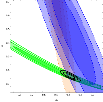
  The $1\sigma$, $2\sigma$ and $3\sigma$ confidence contours in the $q_{0}-q_{1}$ plane are shown for the combined data sets, both with LBT and without LBT data in Fig 1b and Fig 1a respectively. The contours obtained with joint analysis are very tight as compared to the ones obtained with SNe and galaxy clusters. The best fit values of the model parameters and the $z_{t}$ for different data sets are displayed in the table 1 below. The best fit values with 1$\sigma$ errors for (CMB/BAO+Hubble+Union2+LBT) data set and for (CMB/BAO+Hubble+Union2) data set are ($q_{0}=-0.332\pm 0.018$, $q_{1}=0.146\pm 0.011$, $z_{t}=2.27\pm 0.12$) and ($q_{0}=-0.371\pm 0.023$, $q_{1}=0.154\pm 0.011$, $z_{t}=2.4\pm 0.22$) respectively. The value of $w(z)$ at present with $1\sigma$ errors for (CMB/BAO+Hubble+Union2+LBT) data set is $-0.792\pm 0.017$.

  Table 1: Best fit values for first parameterization

  Data Set	$\chi^{2}/d.o.f$	$q_{0}$	$q_{1}$	$q(0)$	$z_{t}$
  CMB/BAO	0.538	$-0.491$	$0.202$	-0.491	2.43
  Union2	0.954	$-0.524$	$0.859$	-0.524	0.61
  Hubble	0.765	$-0.347$	$0.449$	-0.347	0.77
  LBT	0.491	$-0.202$	$0.07$	-0.202	2.88
  CMB/BAO+Union2+Hubble	0.971	$-0.371$	$0.154$	-0.371	2.4
  CMB/BAO+Union2+ Hubble + LBT	1.009	$-0.332$	$0.146$	-0.332	2.27

  Fig.3a and Fig.3c show the evolution of deceleration parameter and equation of state respectively, with redshift $z$. There is a transition from accelerated to decelerated phase. The transition redshift in this model is $z_{t}=2.4$ (with SNe Ia + H(z) + CMB/BAO) and the $z_{t}$ is lower down to 2.2 when LBT data is included in the joint analysis of SNe Ia, H(z) and CMB/BAO. This $z_{t}$ is very high as compare to $\Lambda$CDM prediction ($z_{t}=0.66$). The joint analysis with LBT gives present value of deceleration parameter as $q_{0}=-0.332$.

  

  (a) Part 1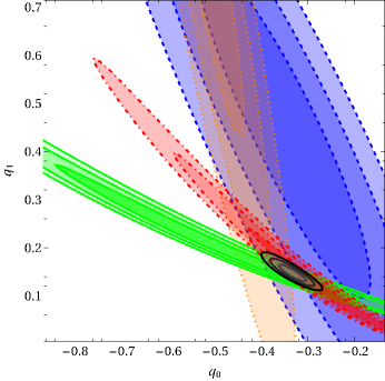

  

  (b) Part 1

  Figure 1: The $1\sigma,2\sigma$ and $3\sigma$ contours in $q_{0}-q_{1}$ for first parameterization. The gray contours are for the combined chi-squared. Green (continuous line) contours correspond to CMB/BAO, red (Dash-dot) curves are for lookback time, orange (Dotted) lines are SNe Ia and blue (Dashed) curves are for Hubble data.

• Parameterization II: $q_{II}(z)=q_{2}+q_{3}(\frac{z}{1+z})$

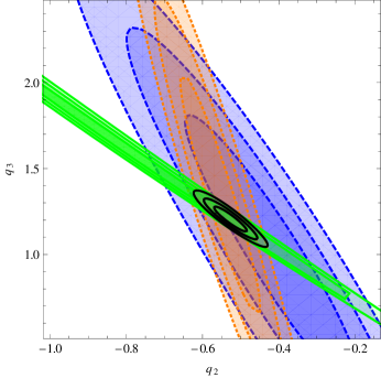
  Confidence regions ($1\sigma$, $2\sigma$ and $3\sigma$) in $q_{2}-q_{3}$ parametric plane for SNe Ia, H(z), CMB/BAO and joint analysis are shown in Fig 2a and Fig. 2b. The best fit values with 1$\sigma$ errors for the (CMB/BAO + Hubble + Union2 + LBT) data set and for (CMB/BAO + Hubble + Union2) are ($q_{2}=-0.595\pm 0.073$, $q_{3}=1.278\pm 0.042$, $z_{t}=0.87\pm 0.20$) and ($q_{0}=-0.526\pm 0.028$ , $q_{3}=1.205\pm 0.046$, $z_{t}=0.77\pm 0.09$) respectively. The value of $w(z)$ at present with $1\sigma$ errors for (CMB/BAO+Hubble+Union2+LBT) data set is $-1.042\pm 0.07$.

  Table 2: Best fit values for second parameterization

  Data Set	${\chi}^{2}/d.o.f$	${q_{2}}$	${q_{3}}$	$q(0)$	$z_{t}$
  CMB/BAO	0.556	$-0.775$	$1.578$	-0.775	0.96
  Union2	0.956	$-0.552$	$1.335$	-0.552	0.70
  Hubble	0.761	$-0.411$	$1.014$	-0.411	0.68
  LBT	0.495	$-0.325$	$0.58$	-0.325	1.27
  CMB/BAO + Union2 + Hubble	0.947	$-0.526$	$1.205$	-0.526	0.77
  CMB/BAO + Union2 + Hubble + LBT	0.957	$-0.595$	$1.278$	-0.595	0.87

  Similarly the joint analysis is further done by the inclusion of LBT for this parameterization, shown in Fig. 2b. The joint analysis with LBT shifts the best fit parameter values towards the higher side. The constraints obtained on the parameter values by the joint analysis are very tight as compared to the constraints obtain from the SNe Ia data and the galaxy cluster data sets independently.

  Fig.3b and Fig.3d display the variation of deceleration parameter and equation of state respectively, w.r.t. the redshift. The reconstruction of the $q(z)$ is done by the joint analysis of SNe Ia + CMB/BAO + LBT + H(z) data sets. The central line is drawn with the best fit values of the model parameters. The transition redshift in this case is, $z_{t}=0.87$.

  

  (a) Part 2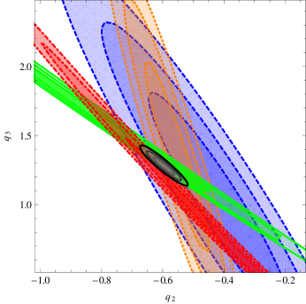

  

  (b) Part 2

  Figure 2: The $1\sigma,2\sigma$ and $3\sigma$ contours in $q_{2}-q_{3}$ plane with all the data sets in case of second parameterization. The gray contours are for the combined chi-squared. Green (continuous line) contours correspond to CMB/BAO, red (Dash-dot) curves are for lookback time, orange (Dotted) lines are SNe Ia and blue (Dashed) curves are for Hubble data.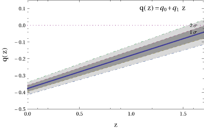

  

  (a) Part 3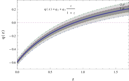

  

  (b) Part 3

  

  (c) Part 3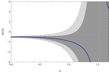

  

  (d) Part 3

  Figure 3: (a) and (b) correspond to variation of q(z) vs z for combined chi-squared for first and second parameterization respectively with $1\sigma$ and $2\sigma$ level. (c) and (d) correspond to variation of $w(z)$ vs z for combined chi-squared for first and second parameterization respectively with $1\sigma$ and $2\sigma$ level. For plotting (c) and (d) the value of $\Omega_{m0}$ is taken to be 0.3.

• Parameterization III: $q_{III}(z)=\frac{1}{2}+\frac{q_{4}}{(1+z)^{2}}$ The best fit values with 1$\sigma$ errors for the (CMB/BAO + Hubble + Union2 + LBT) data set and for (CMB/BAO + Hubble + Union2) are ($q_{4}=-1.296\pm 0.024$, $z_{t}=0.61\pm 0.01$) and ($q_{4}=-1.162\pm 0.03$, $z_{t}=0.52\pm 0.02$) respectively and hence the present value of deceleration parameter equal to $q_{0}=-0.796$ (See Figs 4b and 4a). The value of $w(z)$ at present with $1\sigma$ errors for (CMB/BAO + Hubble + Union2 + LBT) data set is $-1.234\pm 0.023$.

  The best-fit evolution of deceleration parameter and equation of state with redshift is shown in Fig 4c and Fig 4d respectively. The $1\sigma$ error bar in this curve is very tight as compare to the two parameter model of parameterization. The transition redshift in this case is $z_{t}=0.61$ which is in agreement with $\Lambda$ CDM model with in 1$\sigma$ level. The results for single parameter parameterization for the rest of the data sets are summarized in table 3 below.

  Table 3: Best fit values for third parameterization

  Data Set	$\chi^{2}/d.o.f$	$q_{4}$	$q(0)$	$z_{t}$
  CMB/BAO	0.589	$-1.264$	-0.764	0.58
  Union2	0.957	$-1.14$	-0.64	0.51
  Hubble	0.805	$-1.115$	-0.615	0.49
  LBT	0.567	$-1.47$	-0.97	0.71
  CMB/BAO + Union2 + Hubble	0.952	$-1.162$	-0.66	0.52
  CMB/BAO + Union2 + Hubble + LBT	1.028	$-1.296$	-0.79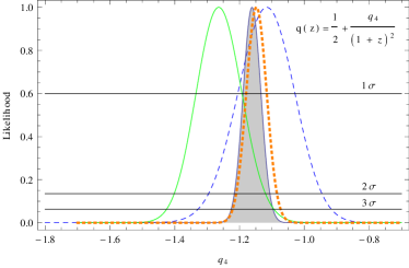6	0.61

  

  (a) Part 4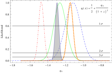

  

  (b) Part 4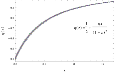

  

  (c) Part 4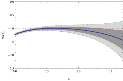

  

  (d) Part 4

  Figure 4: (a) and (b), Likelihood vs parameter plots with all the data sets in case of third parameterization. The filled gray plot are for the combined chi-squared. Green (continuous line) correspond to CMB/BAO, red (Dash-dot) curves are for lookback time, orange (Dotted) lines are SNe Ia and blue (Dashed) curves are for Hubble data. (c) q(z) vs z for combined chi-squared for third parameterization with $1\sigma$ and $2\sigma$ level (d) $w(z)$ vs z for combined chi-squared for third parameterization with $1\sigma$ and $2\sigma$ level. For plotting (c) and (d) the value of $\Omega_{m0}$ is taken to be 0.3.

The summary of the results are the following:

• We have shown that inclusion of LBT in the joint analysis is very important in the measurement of cosmological parameters. This addition of age of passively evolving galaxies as a cosmic clock is completely independent and competitive with standard candles and rulers.

• For all the three parameterizations considered here, the data favors a transition from the deceleration phase to acceleration phase of the Universe. Also, at present our Universe is accelerating. This is also supported by the value of equation of state of dark energy at the present epoch (see Figs 3(c), 3(d) and 4(d)).

• The transition redshift $z_{t}$ strongly depends upon the form of the parameterization of $q(z)$. The transition redshift from decelerated to accelerated expansion ($q(z)=0$) increases with the inclusion of LBT in the analysis except for the parameterization I. Similarly the present value of deceleration parameter become more negative with the inclusion of LBT except for the parameterization I. But the change in the value of $q_{0}$ is small.

• The linear parameterization, $q_{I}$, predicts the transition redshift $z_{t}>2$ which is not compatible with the $\Lambda$CDM model even at $3\sigma$ level. So this model is not reliable at all.

Using SNe Ia data only, Mortsell $\&$ Clarkson (2009) [36] showed that the expansion of Universe is accelerating at low redshifts even at $>12\sigma$ level. In their recent work Xu et al. [37] put bound on model parameters of $q(z)$ by using SNe Ia, BAO and observational H(z) data. Further Lu et al. (2011)[38] again tried to constrain the kinematic model by using the SNe Ia and H(z) data only. They show the two parameterized forms of $q(z)$ clearly deviated from the $\Lambda$CDM model.

It is natural to extend this work with addition of more observational data set like gravitational lensing as a new standard ruler, GRB’s as a standard candles and age of globular clusters as a cosmic chronometers in the present work.

References

- [1] Riess A. G. et al., (Supernova Search Team) Observational evidence from Supernovae for an accelerating Universe and a cosmological constant, Astrophys. J. 116 (1998) 1009, [arXiv:astro-ph/9805201].
- [2] Perlmutter S. et al., (Supernova Cosmology Project) Measurement of Omega and Lambda from 42 high-redshift Supernovae, Astrophys. J. 517 (1999) 565, [arxiv:astro-ph/9812133].
- [3] Astier P. et al., The Supernovae Legacy Survey: measurement of , and from the first year data set, Astron. Astrophys. 447 (2006) 31, [arXiv:astro-ph/0510447].
- [4] Tegmark M. et al., (SDSS) Cosmological parameter from SDSS & WMAP, Phys. Rev. D 69 (2004) 103501, [arXiv:astro-ph/0310723].
- [5] Eisenstein et al., Cosmic Complementarity: and from Combining CMB Experiments and Redshift Surveys, Astrophys. J. 504 (1998) 57, [arXiv:astro-ph/9805239].
- [6] Padmanabhan T., Cosmological constant: The weight of the vacuum, Phys. Rep. 380 (2003) 235 [arXiv:hep-th/0212290]; Copeland E. J., Sami M.& Tsujikawa S., Dynamics of dark energy, Int. J. Mod. Phys. D 15 (2006) 1753 [arXiv:hep-th/0603057]; Sahni V. & Starobinsky A., Reconstructing Dark Energy, Int. J. Mod. Phys. D 15 (2006) 2105 [arXiv:astro-ph/0610026] ; Frieman J. A., Turner M. & Huterer D., Dark Energy and the Accelerating Universe, Ann. Rev. Astron. Astrophys. 46 (2008) 385 [arXiv:0803.0982]; Caldwell R. R. & Kamionkowski M., The Physics of Cosmic Acceleration, Ann. Rev. Nucl. Part. Sci. 59 (2009) 397 [arXiv:0903.0866] ; Li M. et al., Dark Energy, Commun. Theor. Phys 56 (2011) 525.
- [7] Shapiro C. & Turner M., What Do We Really Know About Cosmic Acceleration?, Astrophys. J. 649 (2006) 563, [arXiv:astro-ph/0512586].
- [8] Blandford R. et al., Cosmokinetics, Observing Dark Energy (NOAO/Tucson proceedings), [arXiv:astro-ph/0408279].
- [9] Turner M. & Riess A., Do SNe Ia Provide Direct Evidence for Past Deceleration of the Universe?, Astrophys. J. 569 (2002) 18, [arXiv:astro-ph/0106051].
- [10] Dodelson S. et al., Solving the Coincidence Problem: Tracking Oscillating Energy, Phys. Rev. Lett. 85 (2000) 5276, [arXiv:astro-ph/0002360].
- [11] German G. & de la Macorra A., Lect. Notes Phys 646 (2004) 259.
- [12] Riess A. G. et al., (Supernova Search Team), Type Ia Supernova Discoveries at From the Hubble Space Telescope: Evidence for Past Deceleration and Constraints on Dark Energy Evolution, Astrophys. J. 607 (2004) 665, [arXiv:astro-ph/0402512].
- [13] Komatsu E. et al., Five-Year Wilkinson Microwave Anisotropy Probe Observations: Cosmological Interpretation, Astrophys. J. Suppl. 180 (2009) 330, [arXiv:0803.0547].
- [14] Saini T. D. et al., Reconstructing the cosmic equation of state from supernova distances, Phys. Rev. Lett. 85 (2000) 1162, [arXiv:astro-ph/9910231].
- [15] Simon J., Verde L. & Jimenez R., Constraints on the redshift dependence of the dark energy potential, Phys. Rev. D 71 (2005) 123001, [arXiv:astro-ph/0412269].
- [16] Dantas M. A., Alcaniz J. S. Jain D. & Dev A., Age constraints on the cosmic equation of state, Astron. Astrophys. 467 (2007) 421, [arXiv:astro-ph/0607060].
- [17] Stern D. et al., Cosmic chronometers: constraining the equation of state of dark energy. I: H(z) measurements, JCAP 1002 (2010) 008, [arXiv:0907.3152].
- [18] Gaztanaga E., Cabr A. & Hui A., Clustering of luminous red galaxies - IV. Baryon acoustic peak in the line-of-sight direction and a direct measurement of H(z), Mon. Not. Roy. Astr. Soc. 399 (2009) 1663, [arXiv:0807.3551].
- [19] Chen Y.& Ratra B., Hubble parameter data constraints on dark energy, [arXiv:1106.4294].
- [20] Zhang T. J. et al., Constraints on the Dark Side of the Universe and Observational Hubble Parameter Data, Adv. Astron (2010) 184284, [arXiv:1010.1307].
- [21] Ma C. & Zhang T. J., Power of Observational Hubble Parameter Data: A Figure of Merit Exploration, Astrophys. J. 730 (2011) 74, [arXiv:1007.3787].
- [22] Amanullah R. et al., Spectra and Light Curves of Six Type Ia Supernovae at 0.5111.12 and the Union2 Compilation, Astrophys. J. 716 (2010) 712, [arXiv:1004.1711].
- [23] Cooray A. et al., Measuring Angular Diameter Distances through Halo Clustering Astrophys. J. Lett. 557 (2001) 7, [arXiv:astro-ph/0105061].
- [24] Blake C. et al., The WiggleZ Dark Energy Survey: mapping the distance-redshift relation with baryon acoustic oscillations, [arXiv:1108.2635].
- [25] Blake C. et al., The WiggleZ Dark Energy Survey: testing the cosmological model with baryon acoustic oscillations at z=0.6, [arXiv:1105.2862].
- [26] Percival W. J. et al., Baryon acoustic oscillations in the Sloan Digital Sky Survey Data Release 7 galaxy sample, Mon. Not. Roy. Astr. Soc. 401 (2010) 2148, [arXiv:0907.1660].
- [27] Beutler F. et al., The 6dF Galaxy Survey: baryon acoustic oscillations and the local Hubble constant, Mon. Not. Roy. Astr. Soc. 416 (2011) 3017, [arXiv:1106.3366].
- [28] Komatsu E. et al., Seven-year Wilkinson Microwave Anisotropy Probe (WMAP) Observations: Cosmological Interpretation, Astrophys. J. Suppl. 192 (2011) 18, [arXiv:1001.4538].
- [29] Sivia D. S., Data analysis: A Bayesian tutorial, Oxford Science Publication.
- [30] Elgaroy O. & Multamaki T., Bayesian analysis of Friedmannless cosmologies, JCAP 9 (2006) 2, [arXiv:astro-ph/0603053].
- [31] Gong Y. & Wang A., Observational constraints on the acceleration of the Universe, Phys. Rev. D 73 (2006) 083506, [arXiv:astro-ph/0601453].
- [32] Cunha J. V. & Lima J. A. S., Transition redshift: new kinematic constraints from supernovae, Mon. Not. Roy. Astr. Soc. 390 (2008) 210, [arXiv:0805.1261].
- [33] Guimaraes A.C.C., Cunha J.V. & Lima J.A.S., Bayesian Analysis and Constraints on Kinematic Models from Union SNIa, JCAP 10 (2009) 010, [arXiv:0904.3550].
- [34] Rapetti D. et al., A kinematical approach to dark energy studies, Mon. Not. Roy. Astr. Soc. 375 (2007) 1510, [arXiv:astro-ph/0605683].
- [35] Holanda R.F.L. et al., Accessing the Acceleration of the Universe with Sunyaev-Zel’dovich and X-ray Data from Galaxy Clusters, [arXiv:1103.2688].
- [36] Mortsell E. & Clarkson C., Model independent constraints on the cosmological expansion rate, JCAP 01 (2009) 44, [arXiv:0811.0981]
- [37] Xu L. et al., Constraints on Kinematic Model from Recent Cosmic Observations: SNe Ia, BAO and Observational Hubble Data, JCAP 07 (2009) 031, [arXiv:0905.4552].
- [38] Lu J. et al., Constraints on kinematic models from the latest observational data, Phys. Letts. B 699 (2011) 246, [arXiv:1105.1871].