Photon location in spacetime

Abstract

The NewtonWigner basis of orthonormal localized states is generalized to orthonormal and relativistic biorthonormal bases on an arbitrary hyperplane in spacetime. This covariant formalism is applied to the measurement of photon location using a hypothetical 3D array with pixels throughout space turned on at a fixed time and a timelike 2D photon counting array detector with good time resolution. A moving observer will see these detector arrays as rotated in spacetime but the spacelike and timelike experiments remain distinct.

1 Introduction

In nonrelativistic quantum mechanics the localized states at all positions in space at a fixed time form a basis of Dirac delta-functions. In relativistic quantum mechanics particle localization is a difficult and controversial concept. Photons are always in the relativisitic regime so the problems are especially severe in their case. However, in spite of the theoretical difficulties, localized photon states are a useful concept. The projection operators onto these localized states define a positive operator valued measure (POVM) that has been used to describe photon position in imaging and photon counting experiments [1, 2, 3].

While the probability density basis describes the position of a particle at a fixed time, an experimenter might use a photon counting array detector and record arrival time at one of its pixels. In the nonrelativistic context a spatial volume element is a scalar. In relativity space and time form the four dimensional Minkowski spacetime in which the volume of ordinary space is a spacelike hyperplane with its normal parallel to the time axis. The elements of a photon counting array have normals in a spacelike direction and thus are timelike. Here both possibilities will be combined to give a covariant theory of photon location.

Newton and Wigner (NW) derived bases of localized states at a fixed time for massive particles and zero mass particles with spin zero and one-half [4]. These states are orthogonal and hence localized in the sense that the invariant inner product of states centered at different positions equals zero. The NW procedure failed for photons because spherical symmetry was assumed. However a basis of localized photon states with axial symmetry can be constructed using the NW procedure [5], thus extending the concept of NW localization to photons.

Particle density is usually expressed in terms of the positive frequency part of the field. According to Hegerfeldt’s theorem this leads to instantaneous spreading and possible causality violations [6]. Recent work on the Klein Gordon (KG) equation shows that it is possible to include negative frequency terms and this approach will be applied to the photon here.

The plan of this paper is as follows: Some recent work on the KG particles will be reviewed in Section 2 and extended to the photon in 3. Probability density, photon counting and the perspective of a moving observer will be examined 4 and we will conclude. Rationalized natural units ($\hbar=c=\varepsilon_{0}=\mu_{0}=1$) and covariant notation will be used throughout. An event in spacetime will be described by the four-vector $x=x^{\mu}=\left(t,\mathbf{x}\right)$. With the metric signature $\left(-,+,+,+\right)$, $x_{\mu}=\left(-t,\mathbf{x}\right)$. The four-wavevector is $k^{\mu}=\left(k^{0},\mathbf{k}\right)$. Repeated indices in products of four-vectors will imply summation and a contraction such as $kx=k_{\mu}x^{\mu}=-k^{0}t+\mathbf{k\cdot x}$ is an invariant. Sums over polarization and positive and negative flux directions will be written out explicitly.

2 Klein-Gordon particles

Recent work motivated by attempts to reconcile quantum mechanics with general relativity has lead to a better understanding of the localization of KG particles. A norm that is positive definite for both positive and negative frequencies and zero for their cross terms can be defined as [7, 8, 9]

$$\left\langle\mathbf{k},\varepsilon\mathbf{|k}^{\prime},\varepsilon^{\prime}\right\rangle=2\omega\delta^{3}\left(\mathbf{k}-\mathbf{k}^{\prime}\right)\delta_{\varepsilon,\varepsilon^{\prime}}$$ (1)

where $\omega=\sqrt{\mathbf{k\cdot k}+m^{2}}$ and $\varepsilon=\pm$. The KG field can then be written as

$$\psi_{\varepsilon}\left(x\right)=\int_{k^{0}=\varepsilon\omega}\frac{d^{3}k}{2\omega}\frac{\exp\left(ikx\right)}{\left(2\pi\right)^{3/2}}\psi_{\varepsilon}\left(k\right)$$ (2)

where $\left|\psi\right\rangle$ is a one-particle state vector, $\psi_{\varepsilon}\left(k\right)=\left\langle k,\varepsilon|\psi\right\rangle$ and $k^{0}=\varepsilon\omega$. The invariant inner product defined in [8] is

$$\left\langle\phi|\psi\right\rangle=i\sum_{\varepsilon=\pm}\varepsilon\int_{\Sigma}d\sigma^{\mu}\phi_{\varepsilon}^{\ast}\left(x\right)\stackrel{{\scriptstyle\leftrightarrow}}{{\partial}}_{\mu}\psi_{\varepsilon}\left(x\right)$$ (3)

where

$$f\left(x\right)\stackrel{{\scriptstyle\leftrightarrow}}{{\partial}}_{\mu}g\left(x\right)\equiv f\left(x\right)\partial_{\mu}g\left(x\right)-g\left(x\right)\partial_{\mu}f\left(x\right)$$ (4)

and $\Sigma$ is a hyperplane with normal surface elements $d\sigma^{\mu}$. The integrand in (3) is the KG particle flux across $\Sigma$.

3 Photons

Although (1) is invariant, it will be generalized to an arbitrary hyperplane to allow consistent evaluation of the equations derived here. Also, for photons it is necessary to include polarization $\lambda$. For the special case of planes the reciprocal or $k$-space normals are the same as those in $x$-space so the hyperplanes will still be referred to as $\Sigma$ in $k$-space. Since $m=0$ for photons the components of $k$ are related by the dispersion relation $k^{\mu}k_{\mu}=0$ in vacuum. The invariant $\int d^{4}k\delta^{2}\left(k^{\mu}k_{\mu}\right)$ can be integrated over the component of $k$ normal to $\Sigma$ to give $\int_{\Sigma}d\kappa/2\left|k_{\Sigma}\right|$ where $d\kappa$ is a $k$-space hyperplane element,

$$k_{\Sigma}=k^{\mu}n_{\mu}=\varepsilon\left|k_{\Sigma}\right|$$ (5)

and $n^{\mu}$ is a unit normal to $\Sigma$. The $k$-space orthonormality relation then becomes

$$\left\langle k\mathbf{,}\lambda,\varepsilon\mathbf{|}k^{\prime},\lambda^{\prime},\varepsilon^{\prime}\right\rangle=2\left|k_{\Sigma}\right|\delta^{3}\left(k-k^{\prime}\right)_{\Sigma}\delta_{\lambda,\lambda^{\prime}}\delta_{\varepsilon,\varepsilon^{\prime}}$$ (6)

where the subscript $\Sigma$ on the $\delta$-function indicates that it is valid only on the hyperplane $\Sigma$. The one-photon four-potential in vacuum can be written as

$$\psi_{\varepsilon}^{\mu}\left(x\right)=\sum_{\lambda}\int_{\Sigma,k_{\Sigma}=\varepsilon|k_{\Sigma}|}\frac{d\kappa}{2\left|k_{\Sigma}\right|}e_{\lambda}^{\mu}\left(k\right)\frac{\exp\left(ikx\right)}{\left(2\pi\right)^{3/2}}\psi_{\lambda,\varepsilon}\left(k\right)$$ (7)

where $e_{\lambda}^{\mu}\left(k\right)$ form a basis of polarization unit vectors and

$$\psi_{\lambda,\varepsilon}\left(k\right)=\left\langle k,\lambda,\varepsilon|\psi\right\rangle.$$ (8)

With the generalized orthonormality condition (6), $\varepsilon$ now denotes the direction of photon flux across $\Sigma$. The components of $k$ on $\Sigma$ take continuous values from $-\infty$ to $\infty$ and the dispersion relation then requires that the normal component of $k$ take two values, $\pm\left|k_{\Sigma}\right|$.

Since the electric and magnetic field operators form the second rank tensor $F^{\mu\nu}=\partial^{\mu}A^{\nu}-\partial^{\nu}A^{\mu}$, contraction with the four-potential $A_{\mu}$ in the Lorenz gauge gives the four-vector $J^{\mu}=F^{\mu\nu}A_{\nu}$. The positive frequency four-flux operator was derived in [10]. Using the Coulomb gauge in vacuum for simplicity [10] gives

$$J_{\varepsilon}^{\mu}\left(x\right)=\left\langle\phi\left|i\hat{\mathbf{A}}^{\dagger}_{\varepsilon}\cdot\stackrel{{\scriptstyle\leftrightarrow}}{{\partial}}_{t}\hat{\mathbf{A}}_{\varepsilon},-i\hat{\mathbf{A}}^{\dagger}_{\varepsilon}\times\stackrel{{\scriptstyle\leftrightarrow}}{{\nabla}}\times\hat{\mathbf{A}}_{\varepsilon}\right|\psi\right\rangle.$$ (9)

By inspection it can be seen that the timelike component involves the electric field while the spacelike components require the magnetic field. In the latter the difference in (4) becomes a sum due to the asymmetry of the cross product. Eq. (9) is the four-vector generalization of the KG flux. The four-potential $\psi_{+}^{\mu}\left(x\right)\propto\left\langle 0\left|\hat{A}^{\mu\left(+\right)}\left(x\right)\right|\psi\right\rangle$ replaces the positive frequency part of the invariant KG field.

Since photon and KG flux satisfy the same continuity equation, by analogy (3) should replaced with

$$\left\langle\phi|\psi\right\rangle=\sum_{\varepsilon=\pm}\varepsilon\int_{\Sigma}d\sigma_{\mu}J_{\varepsilon}^{\mu}\left(x\right).$$ (10)

According to the definitions adopted here, when counting photons their direction of crossing is irrelevant and the factor $\varepsilon$ ensures that the particle density on $\Sigma$ is positive regardless of this direction. The sum over $\varepsilon$ in the $J_{\varepsilon}^{0}$ term is a sum over forward and backward in time but propagation of a photon backward in time can be reinterpreted as propagation of an antiphoton forward in time. Negative frequency photon absorption will be seen as photon emission so that each pixel can act as a detector or a source.

Integration of (10) over $d\sigma$ gives

$$\left\langle\phi|\psi\right\rangle=\sum_{\lambda,\varepsilon}\int_{\Sigma,k_{\Sigma}=\varepsilon|k_{\Sigma}|}\frac{d\kappa}{2\left|k_{\Sigma}\right|}\phi_{\lambda,\varepsilon}^{\ast}\left(k\right)\psi_{\lambda,\varepsilon}\left(k\right).$$ (11)

The inner product can be evaluated in $k$-space or $x$-space as discussed [11], but evaluation in $k$-space using (11) is simpler.

4 Spacetime location

Only three of the four components of $k$ can be treated an independent variables. Usually the spacelike components, $\mathbf{k}$, are taken to be independent and a localized basis is defined at a fixed time for all points in space and each polarization $\lambda$. However, a moving observer will not agree that localization of these states is simultaneous so this basis is not invariant. Here covariance is achieved by defining a localized basis on an arbitrary hyperplane.

The generalized NW localized state on $\Sigma$ at $x^{\prime}$ with polarization $\lambda^{\prime}$ and flux direction $\varepsilon^{\prime}$ so that $k_{\Sigma}=\varepsilon^{\prime}|k_{\Sigma}|$ is

$$\chi_{x^{\prime},\lambda^{\prime},\varepsilon^{\prime};\lambda,\varepsilon}\left(k\right)=\sqrt{2\left|k_{\Sigma}\right|}\frac{\exp\left(-ikx^{\prime}\right)}{\left(2\pi\right)^{3/2}}\delta_{\varepsilon,\varepsilon^{\prime}}\delta_{\lambda,\lambda^{\prime}}.$$ (12)

Here the primed indices are fixed while the unprimed indices are summed over in (11). According to the inner product (11) these basis states satsify

$$\left\langle\chi_{x^{\prime\prime},\lambda^{\prime\prime},\varepsilon^{\prime\prime}}|\chi_{x^{\prime},\lambda^{\prime},\varepsilon^{\prime}}\right\rangle=\delta_{\varepsilon^{\prime\prime},\varepsilon^{\prime}}\delta_{\lambda^{\prime\prime},\lambda^{\prime}}\delta^{3}\left(x^{\prime\prime}-x^{\prime}\right)_{\Sigma}.$$ (13)

This implies that these states are localized in the sense originally defined by NW [4]. The projection of an arbitrary state vector onto the localized state (12) is

$$\left\langle\chi_{x^{\prime},\lambda^{\prime},\varepsilon^{\prime}}|\psi\right\rangle=\int_{\Sigma,k_{\Sigma}=\varepsilon^{\prime}|k_{\Sigma}|}d\kappa\frac{\exp\left(ikx^{\prime}\right)}{\left(2\pi\right)^{3/2}}\frac{\psi_{\lambda^{\prime},\varepsilon^{\prime}}\left(k\right)}{\sqrt{2\left|k_{\Sigma}\right|}}.$$ (14)

The $x$-space completeness relation is

$$\sum_{\lambda,\varepsilon}\int_{\Sigma,k_{\Sigma}=\varepsilon|k_{\Sigma}|}d\sigma\left\langle\phi|\chi_{x,\lambda,\varepsilon}\right\rangle\left\langle\chi_{x,\lambda,\varepsilon}|\psi\right\rangle=\left\langle\phi|\psi\right\rangle$$ (15)

as can be verified by substitution of (14) and integration over $d\sigma$ to give (11). Eq. (15) is equivalent to the partition of the identity operator

$$\hat{1}=\sum_{\lambda,\varepsilon}\int_{\Sigma,k_{\Sigma}=\varepsilon|k_{\Sigma}|}d\sigma\left|\chi_{x,\lambda,\varepsilon}\right\rangle\left\langle\chi_{x,\lambda,\varepsilon}\right|$$ (16)

that defines a projection valued measure (PVM) which is a special case of a POVM.

Substitution of (12) in (7) gives

$$\chi_{x^{\prime},\lambda^{\prime},\varepsilon^{\prime};\varepsilon}^{\mu}\left(x\right)=\int_{\Sigma,k_{\Sigma}=\varepsilon^{\prime}|k_{\Sigma}|}\frac{d\kappa}{\sqrt{2\left|k_{\Sigma}\right|}}e_{\lambda^{\prime}}^{\mu}\left(k\right)\frac{\exp\left[ik(x-x^{\prime})\right]}{\left(2\pi\right)^{3}}\delta_{\varepsilon,\varepsilon^{\prime}}$$ (17)

demonstrating that the potential describing a particle localized at $x^{\prime}$ is not itself localized as noted by NW.

Eqs. (11) to (17) are the central results of this paper. In the following subsections they will be applied to probability density and photon counting measurements as seen by stationary and moving observers. The equations can be generalized to allow counting of $N$ photons [3].

4.1 Probability density

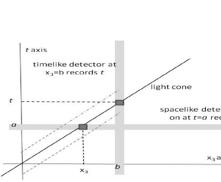
In quantum field theory (QFT) probability density is usually defined at a fixed time $t,$ so that the integrals should be evaluated on a spacelike hyperplane with timelike normal $n^{\mu}=\left(1,0,0,0\right).$ To measure probability density one can imagine an array of transparent detectors throughout space turned on at $t=a$ as sketched as in Fig.1. In this case (14) reduces to

$$\left\langle\chi_{x,\lambda,\varepsilon}|\psi\right\rangle=\int d^{3}k\frac{\exp\left(ikx\right)}{\left(2\pi\right)^{3/2}}\frac{\psi_{\lambda,\varepsilon}\left(k\right)}{\sqrt{2\omega}}.$$ (18)

The probability density is $\sum_{\lambda,\varepsilon}\left\langle\psi|\chi_{x,\lambda,\varepsilon}\right\rangle\left\langle\chi_{x,\lambda,\varepsilon}|\psi\right\rangle$ and the probability to detect a photon is its integral over volume. In spacetime this volume is a hyperpixel with a timelike normal.

Figure 1: Spacetime diagram according to an observer in a reference frame where the experimental apparatii are stationary. The horizontal shaded region depicts a spacelike detector array turned on at a fixed $t$ while the vertical region depicts a timelike photon counting detector at a fixed position, $x_{3}=b.$ The dashed and dot-dash lines parallel to the light cone represent the limits of the photon probability density. For a spacelike (timelike) measurement this terminates on $t=a$ ($x_{3}=b$). The boxes depict the measurement result.

4.2 Photon counting       

Since space and time are on an equal footing in a covariant theory, it is equally valid to fix a spatial coordinate. In fact, this choice describes a planar photon counting array detector with good time resolution. It will be assumed that this detector occupies the plane $x_{3}=b$ with normal $n^{\mu}=\left(0,0,0,1\right)$ parallel to the $x_{3}$-axis as also sketched in Fig. 1. Projection of $\left|\psi\right\rangle$ onto this basis gives

$$\left\langle\chi_{x,\lambda,\varepsilon}|\psi\right\rangle=\int dk_{1}dk_{2}dk^{0}\frac{\exp\left(ikx\right)}{\left(2\pi\right)^{3/2}}\frac{\psi_{\lambda,\varepsilon}\left(k\right)}{\sqrt{2\left|k_{3}\right|}}.$$ (19)

The probability to detect a photon is $\sum_{\lambda,\varepsilon}\left\langle\psi|\chi_{x,\lambda,\varepsilon}\right\rangle\left\langle\chi_{x,\lambda,\varepsilon}|\psi\right\rangle$ integrated over pixel area and measurement time, that is integrated over a hyperpixel with a spacelike normal. If the ”wrong” spacelike probability density basis is used to calculate the flux across a timelike hypersurface an addition factor $cos\theta=k_{3}/\omega$ arises and the formalism is not covariant [14]. The result derived here is more like Fleming’s covariant generalization of the NW basis [15].

If an ideal detector is positioned appropriately relative to the source, the photon will be detected in some hyperpixel of the array with certainty [3]. In writing (19) it was assumed that the $k^{0}$ integral extends from $-\infty$ to $\infty$. For an optical pulse whose line width is small in comparison with its center frequency the negative frequency contributions are negligible, but negative frequencies can be included as discussed previously. The wavevectors $k_{1}$ and $k_{2}$ range from $-\infty$ to $\infty$ but $k_{3}$ takes only the two values $\pm\sqrt{\omega^{2}-k_{1}^{2}-k_{2}^{2}}$. The wavevector component $k_{3}$ can be imaginary. For two points in the plane of the detector $k_{3}$ does not appear in $\left\langle\chi_{x^{\prime\prime},\lambda^{\prime\prime},\varepsilon^{\prime\prime}}|\chi_{x^{\prime},\lambda^{\prime},\varepsilon^{\prime}}\right\rangle,$ but the transition amplitude between arbitrary points does depend on $k_{3}$. The mathematical properties of this Angular Spectrum Representation that includes both propagating and evanescent waves have been studied and it have been applied in optics and acoustics [16].

4.3 Moving observer

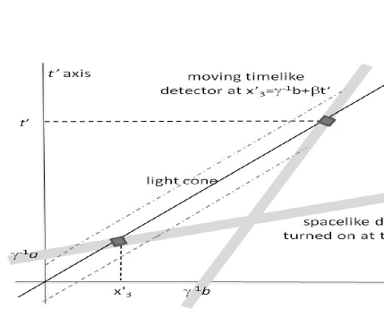
In Fig. 2 the observer is travelling with velocity $-\beta$ relative to the detectors. According to this observer the spacelike photodetector pixels are not turned on simultaneously and the timelike photon counting array is in motion. The detector coordinates are Lorentz transformed to $x^{\prime}_{3}=\gamma(x_{3}+\beta t)$ and $t^{\prime}=\gamma(t+\beta x_{3})$ so that $t^{\prime}=\gamma^{-1}a+\beta x^{\prime}_{3}$ and $x^{\prime}_{3}=\gamma^{-1}b+\beta t^{\prime}$. In the spacelike experiment the observer sees its normal rotated to $n^{\mu}=\left(\gamma,0,0,\gamma\beta\right)$ while the timelike detector is rotated to $n^{\mu}=\left(\gamma\beta,0,0,\gamma\right)$. As $\beta$ approaches unity the light cone $t^{\prime}=x^{\prime}_{3}$ at $\alpha=\tan^{-1}\beta=\pi/4$ is approached so no observer sees a timelike experiment as spacelike and vice versa, but any $n$ has a physical interpretation.

Figure 2: Spacetime diagram as seen by an observer with velocity $-\beta$ relative to the detectors. According to this observer the spacelike hyperpixels are not turned on simultaneously so the detector’s world line makes an angle $\alpha=\tan^{-1}\beta$ with the $x_{3}$-axis. The timelike detector has velocity $\beta$ relative to the $x_{3}$-axis so its world line makes an angle $\alpha$ with the time axis.

5 Conclusion

In this paper it was found that it is possible to define an orthonormal NW basis or a relativistic biorthonormal basis on an arbitrary hyperplane in spacetime. These bases are localized in the sense defined by Newton and Wigner in 1949 [4]: the invariant inner product of two different basis states equals zero. In physical terms projection of the photon state vector onto one of these bases describes a spacelike probability density measurement or a timelike photon counting experiment in which a hyperpixel can act as either a detector or a source. Either family of bases is covariant since a moving observer will just see the hyperplane of the at-rest measurement as rotated in spacetime. Because the observer is limited by the speed of light, the spacelike and timelike experiments are distinct.

Suppose that a source of single photons is available and the location of each photon is to be measured. The basis of localized states at all points in spacetime is vastly overcomplete. The importance of hyperplanes is discussed in [8] and emphasized by Fleming [15]. Here it was demonstrated that a basis can be defined on any fixed hyperplane and that such a basis is complete and exclusive. If a photon exists it should be found somewhere in space at any fixed time (a spacelike experiment). On the other hand an experimentalist is rather more likely to set up a photon counting array detector on some plane in space and wait for the photon to arrive. This is the timelike experiment. In either case it is logical to look for the photon on a fixed hyperplane. Here it was demonstrated that the general case incorporating both these possibilities is a covariant generalization of the NW basis that describes both of these experiments.

Acknowledgements: The author thanks the Natural Sciences and Engineering Research Council for financial support and thanks Juan Leon for valuable discussions.

References

- [1] A. F. Avouraddy, B. E. A. Saleh, A. V. Sergienko, and M. C. Teich, Phys. Rev. Lett. 87, 123601 (2001).
- [2] M. Tsang, Phys. Rev. Lett. 102, 253601 (2009).
- [3] M. Hawton, Phys. Rev. A 82, 012117 (2010).
- [4] T. D. Newton and E. P. Wigner, Rev. Mod. Phys. 21, 400 (1949).
- [5] M. Hawton, Phys. Rev. A 59, 954 (1999); M. Hawton and W. E. Baylis, Phys. Rev. A 71, 033816 (2005).
- [6] G.C.Hegerfeldt, Phys. Rev D 10, 3320-3321 (1974).
- [7] M. Henneaux and C. Teitelboim, Annals Phys. 143, 127 (1982).
- [8] J. Halliwell and M. Ortiz, Phys. Rev. D 48, 748 (1993).
- [9] J. Koksma and W. Westra, arXiv:1012.3473v1 [hep-th] (2010).
- [10] M. Hawton and T. Melde, Phys. Rev. A 51, 4186 (1995).
- [11] M. Hawton, Phys. Rev. A 78, 012111 (2008).
- [12] A. Mostafazadeh, J. Mod Phys. A 21, 2553 (2006).
- [13] M. Hawton, Phys. Rev. A 75, 062107 (2007).
- [14] A. Mostafazadeh and F. Zamani, Annals Phys. 321, 2183 (2006).
- [15] G. N. Fleming, Philosophy of Science 67, 515 (2000).
- [16] E. Wolf, J. Opt. Soc. Am. A 4, 1920 (1986).