Spectral function of few electrons in quantum wires and carbon nanotubes as a signature of Wigner localization

Abstract

We demonstrate that the profile of the space-resolved spectral function at finite temperature provides a signature of Wigner localization for electrons in quantum wires and semiconducting carbon nanotubes. Our numerical evidence is based on the exact diagonalization of the microscopic Hamiltonian of few particles interacting in gate-defined quantum dots. The minimal temperature required to suppress residual exchange effects in the spectral function image of (nanotubes) quantum wires lies in the (sub-) Kelvin range.

After half a century of research, electrons in one dimension still attract attention as a paradigm of interacting behavior that deviates from Fermi liquid theory, exhibiting e.g. spin-charge separation or solid-like order.GiamarchiBook ; Deshpande10 ; Ilani10 This impulse comes from recent experiments in systems with high aspect ratio—cleaved-edge overgrowth structures,Auslander ; Steinberg06 ; Barak10 multiple-gate quantum wires,Hew08 carbon nanotubes,Deshpande08 ; Kuemmeth08 ; Deshpande09 ; Churchill09 ; Steele09 nanowiresRoddaro08 ; Kristinsdottir11 —which are all effectively one-dimensional as their transverse and longitudinal degrees of freedom are decoupled. The refinement of such devices allows to easily reach the dilute regime of electron density yet minimizing the impact of disorder. At sufficiently low density, the Coulomb energy gain overcomes the kinetic energy cost of localization, hence electrons are expected to freeze their motion in space forming a regular array—a Wigner correlated solid.Schulz93 ; Fiete07

So far, the evidence of Wigner localization has ultimately relied on the measure of the energy gap between ground and low-lying excited states, which vanishes in the dilute limit.Steinberg06 ; Deshpande08 ; Steele09 ; Kristinsdottir11 This excitation energy decreases gradually from the liquid- to the solid-like regime, as an effect of both quantum fluctuations and samples’ finite size—systems often act as quantum dots (QDs) in the Coulomb blockade regime.Steinberg06 ; Deshpande08 ; Kuemmeth08 ; Deshpande09 ; Churchill09 ; Steele09 ; Roddaro08 ; Kristinsdottir11 Therefore, an alternative signature of the electron solid, directly related to the wave function, would be desirable. A possible observable is the momentum-resolved spectral function (SF)—the quasiparticle wave function square modulus in reciprocal space.Rontani05 ; Steinberg06 Unpromisingly, it was predicted that the SF was qualitatively similar in both Wigner and non-interacting limitsFiete05 and that any distinctive structure of the SF was washed out by temperature.Mueller05

In this Communication we demonstrate that the space-resolved spectral function of few electrons provides a clear signature of Wigner localization at temperatures above $T_{\text{ex}}$, that is the characteristic scale of exchange interactions. This fundamental observable may be accessed through scanning tunneling spectroscopy (STS).WiesendangerBook ; HoferRMP Our exact diagonalizationBryant87 ; Reimann02 ; Rontani06 ; Secchi09 (ED) results show that the SF resembles the charge density for $T\gtrsim T_{\text{ex}}$, displaying $N$ peaks as the $N$th electron tunnels into a Coulomb blockaded QD already containing $N-1$ electrons. The peak-to-valley ratio of such image allows to assess directly the onset of Wigner localization. In sharp contrast, for $T\ll T_{\text{ex}}$ the SF is system-dependent and unrelated to $N$. Overall, the joint measurements of $N$ and of the SF are able to unveil the Wigner solid.

Figure 1: (Color online) (a-c) SF signal $\cal{G}$ vs $x$ at various $T$ for $N=2\rightarrow N=3$. (a) Quantum wire (QW). The length unit is $\ell_{\text{QD}}=$ 23.9 nm. (b) Carbon nanotube no. 1 (CNT1). $\ell_{\text{QD}}=$ 26.8 nm. (c) Carbon nanotube no. 2 (CNT2). $\ell_{\text{QD}}=$ 17.9 nm. (d) SF signal $\cal{G}$ vs $x$ at $T=$ 10 K for a CNT as $\hbar\omega_{0}$ is varied. The five curves, from red [light gray] to black, correspond to $\hbar\omega_{0}=$ 5, 20, 60, 100, $\infty$ meV, respectively. The length unit is $\ell_{\text{QD}}$ and the remaining parameters are those of CNT2. (e) $T_{\text{ex}}$ vs $\hbar\omega_{0}$ for QW, CNT1, and CNT2. The filled circles are the values pertinent to panels (a-c).

The scenario reported in this Communication agrees with the theory of the ‘spin-incoherent’ Luttinger liquid.Fiete07 On the other hand, crucial approximations of this theory poorly reproduce key experimental features of systems with a moderate number of electrons,Steinberg06 ; Deshpande08 ; Kuemmeth08 ; Deshpande09 ; Churchill09 ; Steele09 ; Roddaro08 ; Kristinsdottir11 and most noticeably: (i) finite-size effects are prominent;Anfuso03 ; Cavaliere04 ; Gindikin07 ; Pugnetti09 ; Schenke09 (ii) the occurrence of the band gapLevitov03 and band curvatureImambekov09 ; Barak10 may not be neglected.

In our ED approach we take into account all many-body correlations as well as the effects of spin-orbit coupling, valley degeneracy, band curvature through the effective mass $m$.Secchi09 We assume the QD confinement potential along $x$ to be harmonic, $V_{\text{QD}}(x)=m\omega_{0}^{2}x^{2}/2$,Reimann02 ; Secchi09 since this is the generic low-energy form for gated QDs embedded in quantum wires (QWs) and semiconducting carbon nanotubes (CNTs), as in Refs. Steinberg06, ; Deshpande08, ; Kuemmeth08, ; Deshpande09, ; Churchill09, ; Steele09, . We consider $N$ electrons in a QW interacting through a screened Coulomb interaction $V(x,x^{\prime})=e^{2}\epsilon^{-1}[(x-x^{\prime})^{2}+\lambda^{2}]^{-1/2}$, with $\lambda$ being a short-range cutoff and $\epsilon$ the dielectric constant. The CNT Hamiltonian is more complex, due to the presence of valleys K and K^′, spin-orbit coupling, inter- and intra-valley interactions. The interaction potential interpolates between Coulomb and Hubbard-like behavior: see Ref. Secchi09, for details. In all cases we diagonalize the Hamiltonian in the space spanned by the Slater determinants built by filling with $N$ electrons the lowest 60 spin-orbitals in all possible ways.

The outcome of the ED consists in the $i$th excited $N$-body states, $\left|N,i\right>$, and their energies $E^{N}_{i}$. The SF for a given initial state at $T=0$, $A_{N-1,i}(x,\omega)$, is

$$A_{N-1,i}(x,\omega)=\sum_{j}\left|\left<N,j\right|\hat{\Psi}^{\dagger}(x)\left|N\!-\!1,i\right>\right|^{2}\!\!\delta(\hbar\omega-E^{N}_{j}+E^{N-1}_{i}),$$

with $\hat{\Psi}^{\dagger}(x)$ being the operator creating an electron at $x$ and $\hbar\omega$ its resonant tunneling energy, whereas the ground-state charge density is $\varrho(x)=N^{-1}\left<N,0\right|\hat{\Psi^{\dagger}}(x)\hat{\Psi}(x)\left|N,0\right>$. Ideally, the STS differential conductance at vanishing temperature and bias, $dI/dV$, is proportional to $A_{N-1,0}(x,\varepsilon_{F}/\hbar)$, with $\varepsilon_{F}$ being the Fermi energy of the STS tip.noteSTS If the thermal broadening $k_{B}T$ is larger than typical energy spacings,WiesendangerBook $dI/dV$ is proportional to

$${\cal{G}}=\int d\omega\left[-\frac{\partial f(\hbar\omega)}{\partial\omega}\right]A_{T}(x,\omega),$$ (1)

where $f(\cdot)$ is the Fermi distribution function and $A_{T}(x,\omega)$ is the finite-temperature SF,

$$A_{T}(x,\omega)=\frac{1}{Z}\sum_{i}e^{-\beta E^{N-1}_{i}}A_{N-1,i}(x,\omega),$$ (2)

with $\beta=1/(k_{B}T)$ and $Z=\sum_{i}\exp{(-\beta E^{N-1}_{i})}$. In the following we tune $\varepsilon_{F}$ appearing in $f(\cdot)$ to match the $N-1\rightarrow N$ transition between ground states.

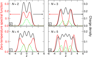
Figure 2: (Color online) QW $\varrho(x)$ of $N$ electrons (black curve) and SF at $T=0$ for the $N-1\rightarrow N$ ground-state transition (solid red [gray] curve) vs $x$ for $N=2$ (a), 3 (b), 4 (c), 5 (d). The dashed curves are the non-interacting SFs, rescaled by a factor 1/6. $A_{N-1,0}(x,\omega)$ is integrated over a tiny energy range around $E^{N}_{0}-E^{N-1}_{0}$. The length unit is $\ell_{\text{QD}}=$ 23.9 nm.

To immediately grasp the key results of this Communication, consider in Fig. 1(c) the SF signal $\cal{G}$ induced by the tunneling of the third electron into a realistic CNT (here labeled CNT2) at various temperatures. At low temperature, $T\ll T_{\text{ex}}=$ 0.017 K, the signal shows two peaks that originate from the symmetries of the ground states. Above $T_{\text{ex}}$ the signal shows three well resolved peaks that resemble the charge distribution of three Wigner-localized electrons [cf. $\varrho(x)$ in Fig. 4(b)]. The peak-to-valley ratio at $T\gg T_{\text{ex}}$ directly measures the degree of spatial localization. This is apparent in Fig. 1(d), as the impact of few-body correlations is reduced by increasing the QD confinement energy $\hbar\omega_{0}$ and hence the ratio of kinetic to Coulomb energy. Whereas for strong correlations (red [light gray] curve) the three peaks are well resolved since electrons separately localize in space, as the interaction is turned off $\cal{G}$ becomes featureless (black curve for $\hbar\omega_{0}=\infty$), clearly discriminating between Wigner and weakly-interacting regimes.

Also the magnitude of $T_{\text{ex}}$ points to electron correlation, the lower the temperature $T_{\text{ex}}$, the stronger the localization. $T_{\text{ex}}$ varies significantly for typical QWs and CNTs as a function of device parameters, like $\hbar\omega_{0}$. In Fig. 1(d) the increase of $\hbar\omega_{0}$ quenches correlations and amplifies the effects of Fermi statistics, raising $T_{\text{ex}}$. For realistic parameters [cf. circles in Fig. 1(d)], we find that $T_{\text{ex}}$ may be as low as 10 mK in some semiconducting CNTs. On the other hand, $T_{\text{ex}}$ is one-two orders of magnitude higher in quantum wires (QWs), $T_{\text{ex}}\sim 1$ K, as an effect of the different impact of screening.

Figure 2 shows $\varrho(x)$ and the zero-temperature SF up to five electrons for a typical wire QD. In the ED we chose $\lambda=$ 5 nm, bulk GaAs parameters, and $\hbar\omega_{0}=$ 2 meV as single-particle energy spacing, providing a characteristic QD length $\ell_{\text{QD}}=(\hbar/m\omega_{0})^{1/2}=23.9$ nm. As it is seen from the spread of $\varrho(x)$ along the axis (black curves in Fig. 2), this corresponds to a typical size of $\approx$ 200 nm for $N=5$, which is comparable to the size $L_{loc}=$ 230 nm of the QD in the dilute limit of Ref. Steinberg06, (Table I). The profiles of $\varrho(x)$ point to the partial localization of the $N$ electrons as $N$ peaks emerge from a featureless liquid droplet. On the other hand, the SFs for the $N-1\rightarrow N$ ground state transitions (solid red [gray] curves in Fig. 2) are qualitatively distinct from $\varrho(x)$ at given $N$. This is patent for $N=3,4,5$, with SFs displaying one, one, and two nodes, respectively, whereas the corresponding $\varrho(x)$’s have no nodes. As seen in Fig. 1(a), ${\cal{G}}$ is insensitive to temperature in the range $T\ll T_{\text{ex}}=$1.1 K, with $k_{B}T_{\text{ex}}$ being the energy splitting between the lowest two-electron triplet and singlet states. Here $k_{B}T_{\text{ex}}$ provides the energy scale of low-lying excitations.

The SFs appearing in Fig. 2 are similar to those obtained in the absence of interaction (dashed lines). In the non-interacting limit the SF is the square modulus of the orbital occupied by the $N$th electron that enters the QD.Rontani05 Such orbital has zero, one, one, and two nodes for $N=2,3,4,5$, respectively, since electrons fill in each orbital level twice due to Kramers degeneracy. As the symmetries of the quantum states do not change in the considered range of interaction, no qualitative differences are seen for the interacting SFs.Fiete05

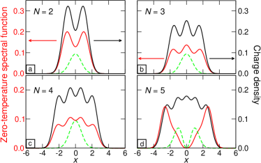
Figure 3: (Color online) CNT $\varrho(x)$ of $N$ electrons (black curve) and SF at $T=0$ for the $N-1\rightarrow N$ ground-state transition (solid red [gray] curve) vs $x$ for $N=2$ (a), 3 (b), 4 (c), 5 (d). The dashed curves are the non-interacting SFs, rescaled by a factor 1/6. $A_{N-1,0}(x,\omega)$ is integrated over a tiny energy range around $E^{N}_{0}-E^{N-1}_{0}$. The length unit is $\ell_{\text{QD}}=$ 26.8 nm.

In the following we discuss two examplar CNT cases. Figure 3 is the analogue of Fig. 2 for the CNT device investigated in Ref. Kuemmeth08, (here labeled as no. 1). The ED parameters ($\hbar\omega_{0}=8$ meV, $\epsilon=3.5$, radius $R=3.6$ nm) were chosen in order to reproduce the measured chemical potentials, as detailed in Ref. Secchi09, . Apart from length renormalization ($\ell_{\text{QD}}=$ 26.8 nm), charge densities (black curves in Fig. 3) are similar to those of the QW (Fig. 2). On the contrary, the zero-temperature SFs for the CNT (solid red [gray] curves in Fig. 3) are drastically different from those of Fig. 2, being all nodeless except for the $N=4\rightarrow N=5$ transition. This trend is qualitatively similar to the non-interacting filling sequence (dashed lines in Fig. 3), as each CNT level is four-fold degenerate in the absence of spin-orbit coupling, due to both spin and valley degeneracies. The spin-orbit interaction splits the multiplet into two doublets (here separated by $\Delta E_{\text{SO}}=$ 0.367 meV) but leaves the spin-orbitals unchanged. Since $\Delta E_{\text{SO}}$ remains the energy scale of the low-lying excitations even in the presence of interactions in the sample no. 1 (Refs. Kuemmeth08, ; Secchi09, ), the SFs of Fig. 3 are unaffected by temperature for $T\ll\Delta E_{\text{SO}}/k_{B}\sim 4$ K [cf. Fig. 1(b)].

The SFs of Figs. 3(a), (b), and (c) display $N$ peaks as the $\varrho(x)$’s, and placed approximately in the same locations. This genuine effect of interaction, reminescent of the partial Wigner localization occuring in the QD, takes place also in the QW [Fig. 2(a)] and it has been observed for the tunneling of the second electron into elongated self-assembled InAs QDs.Maruccio07

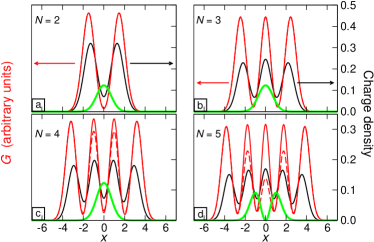
Figure 4: (Color online) SF signal $\cal{G}$ vs $x$ at $T=0.1$ K (dashed curve) and $T=0.5$ K (solid red [gray] and green [light gray] curve) for the CNT QD no. 2. The green [light gray] curve is the non-interacting case. The following $N-1\rightarrow N$ transitions are considered: (a) $N=2$, (b) $N=3$, (c) $N=4$, (d) $N=5$. $\varrho(x)$ for the $N$-body ground state (black curve) is plotted for comparison. The length unit is $\ell_{\text{QD}}=$ 17.9 nm.

The second CNT QD that we study experiences stronger interactions than the first one, as an effect of the smaller energy spacing ($\hbar\omega_{0}=$ 5 meV), dielectric screening ($\epsilon=2.5$), radius ($R=1$ nm). In terms of parameters, the CNT QD no. 2 lies in the middle between the devices investigated in Refs. Deshpande08, and Kuemmeth08, (see Ref. Secchi09, for their placement in a phase diagram). As it is shown in Fig. 4 (black curves), the peak-to-valley ratios of charge densities are about twice as large as those in Figs. 2 and 3, hence electrons are strongly localized.

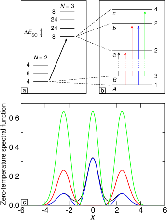
Figure 5: (Color online) SFs of the CNT QD no. 2. (a) Lowest excited states for $N=2$ and $N=3$. The numbers label sub-multiplet degeneracies. (b) Blow-up of panel a (not in scale). Arrows point to allowed tunneling transitions. (c) SFs of allowed transitions vs $x$ at $T=0$. The various $A_{N-1,0}(x,\omega)$ are integrated over tiny energy ranges around the resonance energies highlighted by the arrows in panel b, according to the color [gray tone] code. The length unit is $\ell_{\text{QD}}=$ 17.9 nm.

In this Wigner regime the low-lying excited states are easily thermally populated and are highly degenerate. The reason is that exchange interactions between localized electrons are suppressed ($T_{\text{ex}}$ is only 17 mK), therefore each electron may flip its spin independently from the others at low energy cost.Secchi09 This is true also for the isospin—the orbital angular momentum along $x$ labelling valleys K and K^′. The overall result is that the many excited states which differ only in the (iso)spin value are almost degenerate. This situation is illustrated in Fig. 5(a), where we depict the excited-state ladders for $N=2$ and $N=3$. In the ultimate Wigner limit one expects the ground state to be exactly $4^{N}$ degenerate, as each electron may flip its spin and isospin in four different ways. The effect of spin-orbit interaction (here $\Delta E_{\text{SO}}=$ 1.32 meV) is to split the ground-state multiplet into equally spaced sub-multiplets (three and four for $N=2$ and $N=3$, respectively).

Residual exchange interactions further split the levels, as illustrated by the blow-up of the two lowest sub-multiplets for $N=2$ and $N=3$ shown in Fig. 5(b) (not in scale). For example, states A and B for $N=2$, having the orbital part of the wave function even and odd with respect to reflection symmetry, respectively, by definition are split by $k_{B}T_{\text{ex}}=$ 1.38 $\mu$eV. Similarly, states $a$, $b$, $c$ for $N=3$ have distinct orbital symmetries and are split by 4.45 $\mu$eV ($a$ from $b$) and 2.26 $\mu$eV ($b$ from $c$), respectively.

It is clear that already at $T_{\text{ex}}=17$ mK the excited states of Fig. 5(b) are significantly populated. Therefore, even at low temperatures—say $T=$ 100 mK for state-of-the-art STS—the SF is a statistical mixture of several transitions, explicited in Fig. 5. The arrows depicted in Fig. 5(b) point to the low-energy transitions between $N=2$ and $N=3$ that are allowed by spin, isospin, and orbital symmetries.Secchi09 The corresponding SFs at $T=0$ are shown in Fig. 5(c). Each plot of Fig. 5(c) maps onto a different transition [the arrow of like color (gray tone) in Fig. 5(b)] except the red [light gray] plot which is identical for both $A\rightarrow a$ and $B\rightarrow b$ resonances.

The SFs plotted in Fig. 5(c) differ among themselves with regards to both the number of peaks and their relative intensities. The variations are dictated by the symmetries of initial and final states involved in the tunneling transition. For example, the fundamental transition $A\rightarrow a$ between two- and three-electron ground states displays two peaks located at opposite positions (red [light gray] curve), whereas all other depicted SFs have three peaks each. This shows that the SF at $T=0$ may greatly deviate from the charge-density profile, corroborating the findings of Figs. 2 and 3. On the other hand, the locations of the maxima of curves in Fig. 5(c) coincide.

By statistically averaging the SFs of low-lying transitions, as those shown in Fig. 5(c), one obtains the finite-temperature signal $\cal{G}$ [cf. Eq. (1)]. Figure 4 shows the pattern of $\cal{G}$ at $T=$ 0.1 K (dashed curves) and $T=$ 0.5 K (solid red [gray] curves) for transitions $N-1\rightarrow N$ up to $N=5$. The small dependence of $\cal{G}$ on the temperature exhibited in Figs. 4(c-d) [see differences between dashed and solid red (gray) curves] is a finite-size effect due to the form of the potential $V_{\text{QD}}(x)$, as the electron density slightly increases with $N$ (Ref. Reimann02, ). Remarkably, $\cal{G}$ has a regular behavior as a function of $N$ already at $T=0.5$ K, systematically displaying $N$ peaks of comparable heights whose positions are close to (but non coinciding with) the locations of the maxima of $\varrho(x)$ (black curves).

The pattern of $\cal{G}$ shown in Fig. 4—exhibiting high peak-to-valley ratio—is peculiar of the Wigner regime and should be contrasted with the featureless, non-interacting profile (green [light gray] curves). Indeed, the low-lying excited states, as those of Fig. 5(a), have all roughly the same orbital wave function modulus, similar to the vibrational wave function of nuclei of polyatomic molecules.Secchi09 The differences among orbital states, as well as those among SFs [cf. Fig. 5(c)], originate from the different nodal surfaces. Since the weight is mainly localized around the equilibrium positions of electrons, nodeless interstitial regions may hardly be distinguished from nodal regions. Therefore, the statistical average of excited states shows a regular trend, linked to the positions of localized electrons.

At sufficiently high temperatures, the SF signals $\cal{G}$ of all investigated devices behave similarly. This is shown in Fig. 1 for the tunneling transition $N=2\rightarrow N=3$. Above their respective temperatures $T_{\text{ex}}$, highlighted as circles in Fig. 1(d), all $\cal{G}$ profiles exhibit three peaks of similar height: see the curves for $T=4$, 10, 0.1 K in Figs. 1(a), (b), (c), respectively. The different peak-to-valley ratios of these curves measure the degree of Wigner localization, the lower $T_{\text{ex}}$, the higher the ratio.

At $T\gg T_{\text{ex}}$ the central peak of the QW signal is depleted again [red (light gray) curve for $T=30$ K in Fig. 1(a)], whereas CNT profiles [red (light gray) curves in Figs. 1(b) and (c)] remain stable well above 50 K. This change is due to the excitation of the energy scale associated to charge. In fact, the charging energy of the QW, estimated as the energy difference between the resonance energies of the first two electrons, is $5.1$ meV, that is comparable with 30 K, whereas CNT charging energies are much larger ($\sim 20$ meV).

In conclusion, we have shown that the spatial dependence of the spectral function provides a clear fingerprint for Wigner localization, as the temperature overcomes the energy scale of exchange interactions. This temperature is low enough in both semiconducting carbon nanotubes and quantum wires to make scanning tunneling spectroscopy feasible. This effect has not been seen in past experiments,Venema99 ; Lee04 likely due to metallic screening, as well as to the presence of disorder and scattering from boundaries. We hope our prediction may stimulate further work along this path.

- (1) T. Giamarchi, Quantum Systems in One Dimension (Clarendon Press, Oxford, 2003).
- (2) V. V. Deshpande, M. Bockrath, L. I. Glazman, and A. Yacoby, Nature 464, 209-216 (2010).
- (3) S. Ilani and P. L. McEuen, Ann. Rev. Condens. Mat. Phys. 1, 1-25 (2010).
- (4) O. M. Auslander, H. Steinberg, A. Yacoby, Y. Tserkovnyak, B. I. Halperin, K. W. Baldwin, L. N. Pfeiffer, and K. W. West, Science 308, 88-92 (2005).
- (5) H. Steinberg, O. M. Auslaender, A. Yacoby, J. Qian, G. A. Fiete, Y. Tserkovnyak, B. I. Halperin, K. W. Baldwin, L. N. Pfeiffer, and K. W. West, Phys. Rev. B 73, 113307 (2006).
- (6) G. Barak, H. Steinberg, L. N. Pfeiffer, K. W. West, L. Glazman, F. von Oppen, and A. Yacoby, Nature Phys. 6, 489-493 (2010).
- (7) W. K. Hew, K. J. Thomas, M. Pepper, I. Farrer, D. Anderson, G. A. C. Jones, and D. A. Ritchie, Phys. Rev. Lett. 101, 036801 (2008); 102, 056804 (2009).
- (8) V. V. Deshpande and M. Bockrath, Nature Phys. 4, 314 (2008).
- (9) F. Kuemmeth, S. Ilani, D. C. Ralph, and P. L. McEuen, Nature (London) 452, 448 (2008).
- (10) V. V. Deshpande, B. Chandra, R. Caldwell, D. S. Novikov, J. Hone, and M. Bockrath, Science 323, 106-110 (2009).
- (11) H. O. H. Churchill, A. J. Bestwick, J. W. Harlow, F. Kuemmeth, D. Marcos, C. H. Swertka, S. K. Watson, and C. M. Marcus, Nature Phys. 5, 321-326 (2009).
- (12) G. A. Steele, G. Gotz, and L. P. Kouwenhoven, Nature Nanotech. 4, 363-367 (2009).
- (13) S. Roddaro, A. Fuhrer, P. Brusheim, C. Fasth, H. Q. Xu, L. Samuelson, J. Xiang, and C. M. Lieber, Phys. Rev. Lett. 101, 186802 (2008).
- (14) L. H. Kristinsdóttir, J. C. Cremon, H. A. Nilsson, H. Q. Xu, L. Samuelson, H. Linke, A. Wacker, and S. M. Reimann, Phys. Rev. B 83, 041101(R) (2011).
- (15) H. J. Schulz, Phys. Rev. Lett. 71, 1864 (1993).
- (16) G. A. Fiete, Rev. Mod. Phys. 79, 801-820 (2007).
- (17) M. Rontani and E. Molinari, Phys. Rev. B 71, 233106 (2005).
- (18) G. A. Fiete, J. Qian, Y. Tserkovnyak, and B. I. Halperin, Phys. Rev. B 72, 045315 (2005).
- (19) E. J. Mueller, Phys. Rev. B 72, 075322 (2005).
- (20) R. Wiesendanger, Scanning Probe Microscopy and Spectroscopy (Cambridge University Press, Cambridge, 1994).
- (21) W. A. Hofer, A. S. Foster, and A. L. Shluger, Rev. Mod. Phys. 75, 1287 (2003).
- (22) G. W. Bryant, Phys. Rev. Lett. 59, 1140 (1987); W. Häusler and B. Kramer, Phys. Rev. B 47, 16353 (1993).
- (23) S. M. Reimann and M. Manninen, Rev. Mod. Phys. 74, 1283 (2002).
- (24) M. Rontani, C. Cavazzoni, D. Bellucci, and G. Goldoni, J. Chem. Phys. 124, 124102 (2006).
- (25) A. Secchi and M. Rontani, Phys. Rev. B 80, 041404(R) (2009); ibid. 82, 035417 (2010).
- (26) A. E. Mattsson, S. Eggert, and H. Johannesson. Phys. Rev. B 56, 15615-15628 (1997); F. Anfuso and S. Eggert, ibid. 68, 241301(R) (2003); P. Kakashvili, H. Johannesson, and S. Eggert, ibid. 74, 085114 (2006); I. Schneider, A. Struck, M. Bortz, and S. Eggert, Phys. Rev. Lett. 101, 206401 (2008).
- (27) F. Cavaliere, A. Braggio, M. Sassetti, and B. Kramer, Phys. Rev. B 70, 125323 (2004).
- (28) Y. Gindikin and V. A. Sablikov, Phys. Rev. B 76, 045122 (2007).
- (29) S. Pugnetti, F. Dolcini, D. Bercioux, and H. Grabert, Phys. Rev. B 79, 035121 (2009).
- (30) C. Schenke, S. Koller, L. Mayrhofer, and M. Grifoni, Phys. Rev. B 80, 035412 (2009).
- (31) L. S. Levitov and A. M. Tsvelik, Phys. Rev. Lett. 90, 016401 (2003).
- (32) M. Pustilnik, M. Khodas, A. Kamenev, and L. I. Glazman, Phys. Rev. Lett. 96, 196405 (2006); A. Imambekov and L. I. Glazman, Science 323, 228 (2009).
- (33) The STS tip dynamically alters the local potential seen by electrons in the dot,Fogler06 ; Qian10 ; Westervelt11 possibly affecting Wigner-like correlations, hence it is crucial to make the measurement weakly invasive. This may be achieved by maximizing the tip-dot distance and minimizing the bias voltage, which sets the extrinsic limit of the measurement to the sensitivity to . The intrinsic limit is the condition that the tip spatial resolution, being proportional to the tip-dot distance, is smaller than the average separation between localized electrons.Fogler06
- (34) L. M. Zhang and M. M. Fogler, Nano Lett. 6, 2206 (2006).
- (35) J. Qian, B. I. Halperin, and E. J. Heller, Phys. Rev. B 81, 125323 (2010).
- (36) E. E. Boyd and R. M. Westervelt, Phys. Rev. B 84, 205308 (2011).
- (37) G. Maruccio, M. Janson, A. Schramm, C. Meyer, T. Matsui, C. Heyn, W. Hansen, R. Wiesendanger, M. Rontani, and E. Molinari, Nano Lett. 7, 2701-2706 (2007).
- (38) L. C. Venema, J. W. G. Wildöer, J. W. Janssen, S. J. Tans, H. L. J. Temminck Tuinstra, L. P. Kouwenhoven, and C. Dekker, Science, 283, 52 (1999).
- (39) J. Lee, S. Eggert, H. Kim, S.-J. Kahng, H. Shinohara, and Y. Kuk, Phys. Rev. Lett. 93, 166403 (2004).