Controlling centrality in complex networks

Abstract

Spectral centrality measures allow to identify influential individuals in social groups, to rank Web pages by their popularity, and even to determine the impact of scientific researches. The centrality score of a node within a network crucially depends on the entire pattern of connections, so that the usual approach is to compute the node centralities once the network structure is assigned. We face here with the inverse problem, that is, we study how to modify the centrality scores of the nodes by acting on the structure of a given network. We prove that there exist particular subsets of nodes, called controlling sets, which can assign any prescribed set of centrality values to all the nodes of a graph, by cooperatively tuning the weights of their out-going links. We show that many large networks from the real world have surprisingly small controlling sets, containing even less than $5-10\%$ of the nodes. These results suggest that rankings obtained from spectral centrality measures have to be considered with extreme care, since they can be easily controlled and even manipulated by a small group of nodes acting in a coordinate way.

Modelling social, biological and information-technology systems as complex networks has proven to be a successful approach to understand their function bocca ; arenas ; bbv ; fortunato . Among the various aspects of networks which have been investigated so far, the issue of centrality, and the related problem of identifying the central elements in a network, has remained pivotal since its first introduction. The idea of centrality was initially proposed in the context of social systems, where it was assumed a relation between the location of an individual in the network and its influence and power in group processes bavelas ; wasserman94 . Since then, various centrality measures have been introduced over the years to rank the nodes of a graph according to their topological importance. Centrality has found many applications in social systems wasserman94 , in biology jmbo01 and in man-made spatial networks ba00 ; porta ; spatial .

Among the various measures of centrality, such as those based on counting the first neighbours of a node (degree centrality), or the number of shortest paths passing through a node (betweenness centrality) Freeman79 ; barthelemy , a particularly important class of measures are those based on the spectral properties of the graph PF_spectral . Spectral centrality measures include the eigenvector centrality Bon1 ; Bon3 , the alpha centrality Bon2 , Katz’s centrality Katz and PageRank BrinPage , and are often associated to simple dynamics taking place over the network, such as various kinds of random walks delvenne ; delosrios ; randomwalks . As representative of the class of spectral centralities, we focus here on eigenvector centrality, which is based on the idea that the importance of a node is recursively related to the importance of the nodes pointing to it. Given an unweighted directed graph $G=(V,E)$ with $N=|V|$ nodes and $K=|E|$ links, described by the $N\times N$ adjacency matrix $A$, the eigenvector centrality $\mathbf{c_{0}}$ of $G$ is defined as the eigenvector of $A^{t}$ associated to the largest eigenvalue $\rho_{0}$, which in formula reads $A^{t}\mathbf{c_{0}}=\rho_{0}\mathbf{c_{0}}$ Bon1 ; Bon2 ; Bon3 . If the graph is strongly connected, then the Perron-Frobenius theorem guarantees that $\mathbf{c_{0}}$ is unique and positive. Therefore, $\mathbf{c_{0}}$ can be normalised such that the sum of the components equals 1, and the value of the $i$-th component represents the centrality score of node $i$, i.e. the fraction of the total centrality associated to node $i$. In this Article we show how to change the eigenvector centrality scores of all the nodes of a graph by performing only local changes at node level. As a first step (see the Methods Section) we have proved that, given any arbitrary positive vector $\mathbf{c}\in\mathbb{R}^{N}$, $\mathbf{c}>0$, and $\mathbf{c}\neq\mathbf{c_{0}}$, it is always possible to assign the weights of all the links of a strongly–connected graph $G$ and to construct a new weighted network $G_{\omega}$, with the same topology as $G$ and with eigenvector centrality equal to $\mathbf{c}$:

$$A^{t}_{\omega}\mathbf{c}=\rho\mathbf{c},$$ (1)

where $A_{\omega}$ is the weighted adjacency matrix of $G_{\omega}$.

This is illustrated in Fig. 1 for a graph with $N=4$ nodes and $K=5$ links. In the original unweighted graph $G$, node $2$ is the node with the highest eigenvector centrality, followed in order by node $3$, node $4$, and node $1$. Now, if we have the possibility of tuning the weights of each of the five links, we can set any centrality value to the nodes of the graph. In figure we show, for instance, how to fix the weights of the five links in order to construct: i) a weighted network $G_{\omega}$ in which all nodes have the same centrality score, and ii) even a weighted network $G_{\omega}$ in which the centrality ranking is totally reversed with respect to the ranking in $G$.

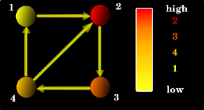
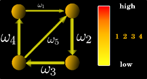
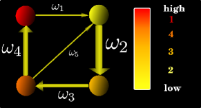
Figure 1: An example of how to tune the link weights to change the node centrality scores. The graph $G$ with $N=4$ nodes and $K=5$ links shown in panel (a) is strongly-connected and has an eigenvector centrality $\mathbf{c}_{0}=\{0.18,0.33,0.27,0.22\}$. By ranking the nodes according to the components of $\mathbf{c}_{0}$, we obtain that node $2$ is the most central one, followed in order by node $3$, node $4$, and node $1$. We can now set the weights of the five links $\bm{\omega}=\{\omega_{1},\omega_{2},\omega_{3},\omega_{4},\omega_{5}\}$ in such a way that Eq.1 is satisfied for any given centrality vector $\mathbf{c}\neq\mathbf{c_{0}}$. For instance, we can get a weighted network $G_{\omega}$ in which all nodes have the same centrality, by solving Eq.1 with a centrality vector $\mathbf{c}=\{1/4,1/4,1/4,1/4\}$ and $\rho=3.0$. We obtain a vector of weights: $\bm{\omega}=\{\alpha,3,3,3,3-\alpha\}$ which, for $0<\alpha<3$, guarantees that all the link weights of the graph are positive. The resulting network $G_{\omega}$ is shown in panel (b). As expected, we have $K-N=1$ free parameter (namely $\alpha$) since the graph has $N=4$ nodes and $K=5$ links. Instead, if we want to reverse the original node ranking we can solve the system $A^{t}_{\omega}\mathbf{c}=\rho\mathbf{c}$ with a centrality vector $\mathbf{c}=\{0.5,0.05,0.2,0.25\}$. Notice that, in this case, the ranking induced by $\mathbf{c}$ is exactly the opposite of the one induced by $\mathbf{c_{0}}$: now node 1 is the most central one, followed in order by node 4, node 3, and node 2. The solution of Eq.2 gives $\bm{\omega}=\{\alpha,12,15/4,6,(3-10\alpha)/5\}$, corresponding to a weighted network $G_{\omega}$ with all positive weights whenever $0<\alpha<3/10$. The resulting network is shown in panel (c).

As shown in the example, given a graph $G$, by controlling the weights of all the links, it is always possible to set any arbitrary vector $\mathbf{c}$ as the eigenvector centrality of the graph. However, tuning the weights of all the $K$ links of a given network is practically unfeasible, especially in large systems. Fortunately, this is not necessary, either. In fact, in the case of Fig. 1, a weighted graph with all nodes having the same centrality score can also be obtained by changing the weights of only four links, while leaving unchanged the weight of the link from node 1 to node 2. More in general, it can be proved that the eigenvector centrality of the whole network can be controlled by appropriately tuning the weights of just $N$ of the $K$ links. The only constraint is that the $N$ links must belong to a subset $E^{\prime}\subseteq E$ such that, for every node $i\in V$, there is a link $\ell\in E^{\prime}$ pointing to $i$ (see Methods Section).

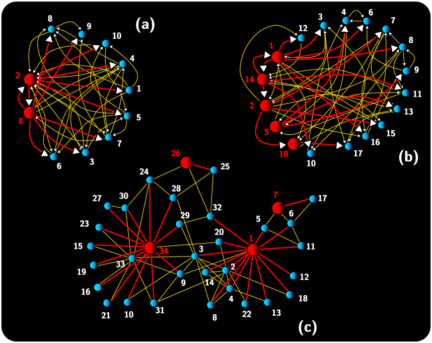
Figure 2: Minimum controlling sets in three real social networks. The graph in panel (a), with $N=11$ vertices and $K=41$ arcs, shows who asks who for an opinion among the members of the student government of the University of Ljubljana in 1992 hlebec . The minimum controlling set is made by the two nodes marked in red, namely node 2 and node 8. These two nodes are linked to each other and point to all the remaining nodes in the graph. Therefore, nodes 2 and 8, by cooperatively modifying the weights of their red links, can set any arbitrary eigenvector centrality to the entire system. The graph in panel (b) has $N=18$ nodes and $K=55$ arcs, and describes the social relations between the monks of an isolated contemporary American monastery, as recorded by Sampson in 1969 sampson . Here, the minimum controlling set contains five nodes, shown in red. In this case, the subset of links $E^{\prime}$ (red links), does not contain links pointing to node 5, so that the red nodes can control the centrality of all the network nodes, except node 5. Finally, the Zachary’s karate club network shown in panel (c) has $N=34$ nodes and $K=78$ undirected edges, and describes the social network of friendships among the members of a US university karate club in 1970 zachary . In this network, the minimum controlling set contains node 1, the instructor Mr. Hi, node 34, the club administrator Mr. John A, and also nodes 7 and 26. Notice that just two nodes, namely 1 and 34, can control the centrality of $95\%$ of the graph nodes.

This is illustrated in Fig. 2 for three real social networks. In each of the three cases, it is possible to set any arbitrary eigenvector centrality by changing only the weights of the red arcs, while keeping unchanged (and equal to $1$) the weights of all remaining arcs, shown in yellow. The nodes from which the links in $E^{\prime}$ originate are also coloured in red, and are referred to as a controlling set of the network (see Methods Section). What is striking is that, in each of the three networks, the set $E^{\prime}$ can be chosen in such a way that all the links in $E^{\prime}$ originate from a relatively small subset of nodes. For instance, the controlling set reported for the student government network of the University of Ljubljana contains only two nodes. This is also a minimum controlling set, since the graph does not admit another controlling set with a smaller number of nodes. This finding indicates that only two members of the student government, namely node 2 and node 8, can in principle set the centrality of all the other members by concurrently modifying the weights of some of their links. It is in fact reasonable to assume that the weight of the directed link from $i$ to $j$, representing in this case the social credit (in terms of reputation, esteem or leadership acknowledgement) given by individual $i$ to individual $j$, can be strengthen or decreased only by $i$. Consequently, nodes 2 and 8 can modify at their will the weights of their out-going links and, If these changes are opportunely coordinated, they can largely alter the actual roles of all the other individuals. Analogously, only five monks can control the centrality of the Sampson’s monk network, while only 4 members of the Zachary’s karate club network can set the eigenvector centrality of the remaining 30 members.

A question of practical interest is to investigate the size ${\cal C}\equiv|C^{*}|$ of the minimum controlling set in various complex networks. When ${\cal C}$ is small with respect to $N$, then the centrality of the network is easy to control. Conversely, when the number of nodes in the minimum controlling set is large, the network $G$ is more robust with respect to centrality manipulations. We have used two greedy algorithms to compute approximations of minimum controlling sets in various real systems (see Methods Section). In Table 1 we report the best approximation for ${\cal C}$, i.e. the size of the smallest controlling set $\overline{C}$ produced by either of the two algorithms in networks whose sizes range from hundreds to millions of nodes. In the majority of the cases we have found unexpectedly small controlling sets, containing only up to $10-20\%$ of the nodes of the network. For instance, in the graph of Jazz musicians, there exists a controlling set made by just $16$ of the $198$ musicians. These $16$ individuals alone can, in principle, decide to set the popularity of all the other musicians, enhancing the centrality of some of the nodes and decreasing the centrality of others, just by playing more or less often with some of their first neighbours. Among all the networks we have considered, the one with the smallest controlling set is the Wikipedia talk communication network, a graph with 2,394,385 nodes in which just $2\%$ of nodes are able to alter the centrality of the entire system. The quantities in parenthesis indicate that for this network a set of just $1\%$ of the nodes can control the centrality of $99\%$ of the nodes.

Network	$N$	$\langle k\rangle$	$\mathcal{C}(G)$	$\mathcal{C}(G^{rnd})$
Web (Berkley and Stanford) leskovec-lang	654782	22.2	8% (3%$\rightarrow$95%)	12%
Web (Google) leskovec-lang	875713	11.1	15% (9%$\rightarrow$94%)	22%
Web (NotreDame) webnd	325729	9.2	13% (8%$\rightarrow$95%)	21%
Web (Stanford) leskovec-lang	281904	16.4	8% (3%$\rightarrow$95%)	15%
Jazz musicians danonjazz	198	27.7	8% (5%$\rightarrow$97%)	13%
Movie actors actors	392340	7.2	11% (8%$\rightarrow$97%)	22%
Cond-Mat coauthorship Newman2001	12722	6.3	23%(18%$\rightarrow$93%)	29%
AstroPh coauthorship Newman2001	13259	18.7	16% (10%$\rightarrow$94%)	27%
Networks coauthorship newman-net	379	4.8	20% (15%$\rightarrow$94%)	29%
URV email urv-email	1133	9.6	23% (16%$\rightarrow$91%)	27%
ENRON email leskovec-lang ; enron	2351	118.7	7%(4%$\rightarrow$97%)	8%
Email EU-All leskovec-kleinberg	265214	3.5	16% (1%$\rightarrow$85%)	26%
Wiki-talk leskovec-hutt	2394385	4.20	2% (1%$\rightarrow$99%)	23%
Hep-Ph citation leskovec-kleinberg	34401	12.25	16% (10%$\rightarrow$94%)	22%
Hep-Th citation leskovec-kleinberg	27400	12.7	17%(8%$\rightarrow$91%)	22%
Patents leskovec-kleinberg	3774768	8.75	50% (16%$\rightarrow$60%)	26%
Internet AS InternetAS	11174	4.2	9% (8%$\rightarrow$99%)	22%
US Airports  USAirports	500	11.9	14% (12%$\rightarrow$97%)	19%
US Power Grid watts	4941	5.33	33% (29%$\rightarrow$95%)	23%
roadnet CA leskovec-lang	1965206	5.63	31% (30%$\rightarrow$96%)	23%
roadnet PA leskovec-lang	1088092	5.67	33% (30%$\rightarrow$967%)	23%
roadnet TX leskovec-lang	1379917	5.57	33% (30%$\rightarrow$97%)	23%
Electronic circuit (s208 st) Alon	123	3.1	29% (26%$\rightarrow$96%)	28%
Electronic circuit (s420 st) Alon	253	3.1	29% (25%$\rightarrow$96%)	28%
Electronic circuit (s838 st) Alon	513	3.2	29% (25%$\rightarrow$96%)	28%
Wordnet wordnet	77595	3.44	26% (19%$\rightarrow$92%)	26%
USF Words associations usf-norms	10618	13.6	22% (8%$\rightarrow$56%)	25%
PGP pgp	10680	4.5	22% (18%$\rightarrow$77%)	29%
Amazon amazon	410236	16.36	17% (9%$\rightarrow$91%)	17%
Epinions epinions	75879	13.41	22% (19%$\rightarrow$95%)	18%
Gnutella leskovec-kleinberg ; gnutella2	62586	4.72	19%(11%$\rightarrow$62%)	31%
PolBlogs polblogs	1224	31.2	13% (8%$\rightarrow$94%)	18%
PolBooks polbooks	105	8.4	15% (12%$\rightarrow$98%)	22%
Slashdot leskovec-lang	82168	23.08	25% (21%$\rightarrow$58%)	27%
Wiki-vote leskovec-hutt	8298	25.00	16% (15%$\rightarrow$99%)	20%

Table 1: Number of nodes $N$, average degree $\langle k\rangle$, and the relative size ${\cal C}(G)$ of the mimimum controlling set found in 35 different real world networks. The values of ${\cal C}(G)$ reported are expressed as percentage of the network size $N$. The algorithms used to find approximations of minimum controlling sets, mark as controllers also nodes not controlling other nodes, simply because, at a certain iteration of the greedy procedure, they have remained with no out-going links. Therefore, we also report in parenthesis the relative size of the effective minimum controlling set and the percentage of the controlled nodes. The notation $x\%\rightarrow y\%$, indicates that $x\%$ of the nodes is able to control the centrality of $y\%$ of the network. In the rightmost column we report, for each network, the relative size of the controlling set in randomized versions which preserve the original degree sequence. We have considered averages over 100 different randomizations. From top to bottom, the networks are divided into six classes, respectively World-Wide-Web, collaboration/communication, citation, spatial, words and socio–economical networks.

For each real network $G$, we have also computed the typical size $\mathcal{C}(G^{rnd})$ of the minimum controlling set in its randomised counterpart (see the rightmost column in Table 1). In particular, we have considered a randomisation which preserves the degree sequence of the original graph. In most of the cases $\mathcal{C}(G)\leq\mathcal{C}(G^{rnd})$, relevant exceptions being some spatial man-made networks, such as power grids, road networks and electronic circuits, and also the patents citation network. This fact suggests that, in the absence of other limitations, such as strong spatial/geographic constraints spatial , the structure of real networks has naturally evolved to favour the control of spectral centrality by a small group of nodes. To better compare the controllability of networks with different sizes, we report in Fig. 3 the ratio $\frac{\mathcal{C}(G)}{\mathcal{C}(G^{rnd})}$ as a function of the number of graph nodes $N$. The smallest values of the ratio $\frac{\mathcal{C}(G)}{\mathcal{C}(G^{rnd})}$ are found for collaboration/communication systems, WWW and socio-economical networks. The five most controllable networks are respectively Wiki-talk, Internet at the AS level, movie actors, the Stanford World Wide Web, and the collaboration network of researchers in astrophysics. These are all networks in which single nodes can tune, at their will, the weights of their out-going links. A scientist can decide whether to weaken or strengthen the connections to some of the collaborators. The administrators of an Internet Autonomous System can control the routing of traffic through neighbouring ASs, by modifying peering agreements vespignani_book . And, similarly, the owner of a Web page can change the weights of hyperlinks, for instance by assigning them different sizes, colour, shapes and positions in the Web page.

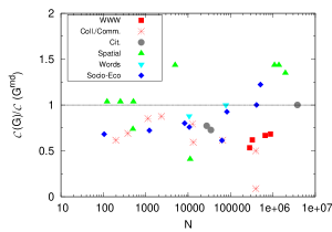
Figure 3: Relative size of the minimum controlling set in various real systems. We report, as a function of $N$, the ratio between the sizes of the minimum controlling set in real networks and in their respective randomized versions (we have considered averages over 100 different realizations). Different symbols and colors refer to the six network classes considered in Table 1. The observed ratio is lower than 1 in most of the cases, with the smallest values corresponding to collaboration/communication systems, WWW and socio-economical networks. The ratio is equal to 1 in three cases. The networks with ratio larger than 1, with the exception of one socio-economical system (namely Epinions), are all spatially constrained systems: three electronic circuits, the US power grid, and three road networks.

In this work, we have shown how a small number of entities, working cooperatively, can set any arbitrary eigenvector centrality for all the nodes of a real complex network. It is straightforward to extend our results to other spectral centralities, such as $\alpha$-centrality and Katz’s centrality. Similar arguments can also be applied, with some limitations, to PageRank: in this case, the inverse centrality problem has solutions only for some particular choices of ${\bf c}$. Such findings suggest that rankings obtained from centrality measures should be taken into account with extreme care, since they can be easily controlled and even distorted by a small group of cooperating nodes. The high controllability of real networks potentially has large social and commercial impact, given that centrality measures are nowadays extensively used to identify key actors, to rank Web pages, and also to assess the value of a scientific research.

I Methods

I.1 Solution to the inverse centrality problem.

The set of $N$ linear equations with $K$ variable weights, $\omega_{1},\ldots,\omega_{K}$, in Eq. 1 can be rewritten as a system of $N$ linear equations with $K$ variables:

$$B\bm{\omega}=\rho\mathbf{c},$$ (2)

where now $B$ is a $N\times K$ matrix of real numbers, and $\bm{\omega}\equiv\{\omega_{1},\ldots,\omega_{K}\}$. Notice that the linear system in Eq. 2 has solutions since the rank of $B$ is $N<K$ (all the equations are separated and each of the variables, $\omega_{1},\ldots,\omega_{K}$, appears in one equation only), and the in-degree of all nodes is positive by definition. Hence, there always exists $\bm{\omega}\in\mathbb{R}^{K}$ such that Eq. 1 is satisfied. It is convenient to rewrite Eq. 2 in a form that emphasises the dependence of matrix $B$ from $c$. We choose to label the arcs as follows: $(i,l)$, $l=1\ldots k^{in}_{i}$ denotes the $l$-th arc entering node $i$, where $k^{in}_{i}$ is the in–degree of node $i$. Likewise, $S_{i,l}$ is the source of arc $(i,l)$, while $\omega_{i,l}$ is the corresponding weight. Using this notation, the $i$-th component of Eq. 2 can be written as:

$$\sum_{l=1}^{k^{in}_{i}}\omega_{i,l}c_{S_{i,l}}=\rho c_{i}$$ (3)

By direct computation, one positive solution of Eq. 3 is given by

$$\omega_{i,1}=\omega_{i,2}=\cdots=\omega_{i,k^{in}_{i}}=\frac{\rho c_{i}}{\sum_{l=1}^{k^{in}_{i}}c_{S_{i,l}}}$$ (4)

where $i=1\ldots N$, and by continuity there are infinite many solutions such that $\omega_{i,l}$ are all positive. In particular, if for node $i$ we have $k^{in}_{i}=1$, then the $i$-th equation of Eq. 3 has a unique solution, while if $k^{in}_{i}>1$, there are always infinitely many solutions depending on $k^{in}_{i}-1$ parameters. Summing up, Eq. (2) has only one solution if all the node in-degrees are equal to one, while there are, in general, infinitely many solutions depending on $K-N$ parameters. Notice that $\rho$ can be different from $\rho_{0}$, meaning that it is also possible to set the value of the largest eigenvalue of the weighted graph.

I.2 Tuning a subset of the graph links.

Here, we show that it is not necessary to fix the weights of all the graph links in order to get an arbitrary centrality vector $\mathbf{c}>0$. In fact, given a subset of links $E^{\prime}\subseteq E$ containing at least one incoming link for each node, it is sufficient to assign some positive weights $\tilde{\omega}(\ell^{\prime})$ to each $\ell^{\prime}\in E^{\prime}$, while keeping $\omega(\ell)$ constant $\forall\ell\in E\setminus E^{\prime}$, for instance all equal to $1$, such that the resulting weighted graph has eigenvector centrality equal to $\mathbf{c}$. Without loss of generality we can assume that the first $k^{c}_{i}>0$ incoming links of each node $i$ belong to $E^{\prime}$, so that the components of Eq. 3 can be written as:

$$\sum_{l=1}^{k^{c}_{i}}\omega_{i,l}c_{S_{i,l}}=\rho c_{i}-\sum_{l=k^{c}_{i}+1}^{k^{in}_{i}}\omega_{i,l}c_{S_{i,l}},\quad i=1\ldots N$$ (5)

Therefore, since $c_{i}>0$ for each $1\leq i\leq N$, then there is a $\rho_{0}>0$ such that for every $\rho>\rho_{0}$

$$\rho c_{i}-\sum_{l=k^{c}_{i}+1}^{k^{in}_{i}}\omega_{i,l}c_{S_{i,l}}>0,\quad i=1\ldots N$$ (6)

and hence, by a similar continuity argument as above, we can ensure that there are infinitely many positive solutions to Eq.5.

I.3 Finding minimum controlling sets.

A controlling set of graph $G$ is any set of nodes $C\subseteq V$ such that:

$$V=C\cup\left(\bigcup_{i\in C}\{j\in V:\enspace e_{ij}\in E\}\right).$$ (7)

This means that, for each node $j$ in the graph, at least one of the two following conditions holds: a) $j\in C$, or b) $j$ is pointed by at least one node in $C$. We use $|C|$ to denote the size of the controlling set, i.e. the number of nodes contained in $C$. Finding the minimum controlling set $C^{*}$ of a graph $G$, i.e. a controlling set having minimal size, is equivalent to computing the so-called domination number of $G$. The domination number problem is a well known NP-hard problem in graph theory west . Therefore, the size of the minimum controlling set can be determined exactly only for small $N$ graphs as those in Fig. 2. To investigate larger graphs we have used two greedy algorithms. The first algorithm, called Top–Down Controller Search (TDCS), works as follows. We initially set $G_{t=0}=G$. We select the node $i_{0}$ with the maximum out-degree in $G_{t=0}$, and mark it as controller node. Then, all the nodes in the out-neighbourhood of $i_{0}$ are marked as controlled and are removed from $G_{t=0}$, together with $i_{0}$ itself. In this way, we obtain a new graph $G_{t=1}$, and we store the controller node $i_{0}$, together with the list of nodes controlled by $i_{0}$. Notice that, removing a generic node $j$ from $G_{t=0}$, also implies that $G_{t=1}$ does not contain any of the links pointing to $j$ or originating from it. The same procedure is iteratively applied to $G_{t=1}$, $G_{t=2}$ and so on, until all the nodes of $G$ are either marked as controller or as controlled nodes. The algorithm produces a set $\overline{C}=\{i_{0},i_{1},i_{2},\ldots\}$, with $|\overline{C}|\geq|C^{*}|$, which is a controlling set of $G$ by construction. The second algorithm is called Bottom–Up Controller Search (BUCS), and it works as follows. We set $G_{t=0}=G$ and consider the set $M(0)$ containing all the nodes in $G_{t=0}$ with minimum in–degree. For each node $i\in M(0)$, we consider the set of nodes pointing to $i$ and select from this set the node $m_{i}$ with the maximal out–degree. This node is marked as controller. Then we obtain a new graph $G_{t=1}$ by removing from $G_{t=0}$ all the controller nodes $m_{i}$ for all $i\in M(0)$, together with all the nodes, marked as controlled, pointed by them. The same procedure is iteratively applied to $G_{t=1}$, $G_{t=2}$ and so on, until all the nodes of $G$ are either marked as controller or as controlled nodes. If a graph $G_{t}$ contains isolated nodes, these are marked as controller and removed from $G_{t}$. The algorithm finally produces a set $\overline{C}=\{i_{0},i_{1},i_{2},\ldots\}$ which is a controlling set of $G$ by construction. We have verified that the controlling sets obtained by both TDCS and BUCS for each of the networks considered are much smaller than those obtained by randomly selecting the controlling nodes. Moreover, the set of controller nodes found by TDCS is in general different from that obtained on the same network by BUCS. Also the sizes of the two controlling sets obtained by the two algorithms are different. In particular, we have noticed that in assortative (disassortative) networks the controlling set produced by TDCS is smaller (larger) than that produced by BUCS.

References

- (1) Boccaletti, S., Latora, V., Moreno, Y., Chavez, M., Hwang, D.U., Complex networks: structure and dynamics. Phys. Rep. 424, 175-308 (2006).
- (2) Arenas, A., Díaz-Guilera, A., Khurths, J., Moreno, Y., Zhou, C. Synchronization in complex networks. Phys. Rep. 469, 93-153 (2008).
- (3) Barrat, A., Barthélemy, M., Vespignani, A. Dynamical Processes in Complex Networks. (Cambridge University Press, Cambridge, 2008).
- (4) Fortunato, S. Community detection in graphs.Phys. Rep. 486, 75-174 (2010).
- (5) Bavelas, A. A mathematical model for group structures. Hum. Organ 7, 16 (1948).
- (6) Wasserman, S., Faust, K. Social Networks Analysis. (Cambridge University Press, Cambridge, 1994).
- (7) Jeong, H., Mason, S.P., Barabási, A.-L., Oltvai, Z. N. Lethality and centrality in protein networks. Nature 411, 41-42 (2001).
- (8) Albert, R., Jeong, H., Barabási, A.-L. Error and attack tolerance of complex networks. Nature, 406, 378-382 (2000).
- (9) Crucitti, P., Latora, V., Porta, S. Centrality measures in spatial networks of urban streets. Phys. Rev. E 73, 036125 (2006).
- (10) Barthélemy, M. Spatial Networks, Phys. Rep. 499, 1-101 (2011).
- (11) Freeman, L.C. Centrality in social network. Conceptual clarification. Social Networks 1, 215-239 (1979).
- (12) Barthélemy, M. Betweenness centrality in large complex networks. Eur. Phys. J. B 38, 163-168 (2004).
- (13) Perra, N., Fortunato, S. Spectral centrality measures in complex networks. Phys. Rev. E 78, 036107 (2008).
- (14) Bonacich, P. Factoring and weighting approaches to status scores and clique identification. J. Math. Soc. 2, 113 (1972).
- (15) Bonacich, P., Lloyd, P. Eigenvector-like measures of centrality for asymmetric relations. Soc. Netw. 23, 191-201 (2001).
- (16) Bonacich, P. Power and centrality: a family of measures. Am. J. Sociol. 92, 1170-1182 (1987).
- (17) Katz, L. A new status index derived from sociometric analysis. Psychometrika 18, 39-43 (1953).
- (18) Brin, S., Page, L. The anatomy of a large-scale hypertextual Web search engine. Comput. Netw. 30, 107-117 (1998).
- (19) Delvenne, J.-C., Libert, A.-S. Centrality measures and thermodynamic formalism for complex networks. Phys. Rev. E 83, 046117 (2011).
- (20) Gfeller, D., De Los Rios, P. Spectral Coarse Graining of Complex Networks. Phys. Rev. Lett. 99, 038701 (2007).
- (21) Fortunato, S., Flammini, A., Random walks on directed networks: the case of PageRank, Int. J. Bifurcat. Chaos 17, 2343-2353 (2007).
- (22) Hlebec,V. Recall versus recognition: comparison of the two alternative procedures for collecting social network data. Developments in Statistics and Methodology, p. 121-129. (A. Ferligoj, A. Kramberger, editors) Metodološki zvezki 9, FDV, Ljubljana, 1993,
- (23) Breiger, R., Boorman, S., Arabie, P. An algorithm for clustering relational data with applications to social network analysis and comparison with multidimensional scaling. J. Math. Psychol. 12, 328-383 (1975).
- (24) Zachary, W. W. An information flow model for conflict and fission in small groups. J. Anthropol. Res. 33, 452-473 (1977).
- (25) West, D.B. Introduction to Graph Theory. (Prentice-Hall, 2nd edition, NJ, 2001).
- (26) Pastor-Satorras, R., Vespignani, A. Evolution and Structure of the Internet: A Statistical Physics Approach (Cambridge University Press, Cambridge, 2004).
- (27) Leskovec, J., Lang, K., Dasgupta, A., Mahoney, M. Community structure in large networks: natural cluster sizes and the absence of large well-defined clusters. arXiv.org:0810.1355, (2008).
- (28) Albert, R., Jeong, H., Barabási, A.-L. Diameter of the World Wide Web. Nature, 401, 130 (1999).
- (29) Gleiser, P., Danon, L. Community Structure in Jazz. Adv. Complex Syst. 6, 565 (2003).
- (30) Barabási, A.-L., Albert, R., Emergence of scaling in random networks. Science 286, 509 (1999).
- (31) Newman, M.E.J. Scientific collaboration networks. II. Shortest paths, weighted networks, and centrality. Phys. Rev. E 64, 016132 (2001).
- (32) Newman, M.E.J. Finding community structure in networks using the eigenvectors of matrices. Phys. Rev. E 74, 036104 (2006).
- (33) Guimera, R., Danon, L., Díaz-Guilera, A., Giralt, F., Arenas, A. Self-similar community structure in a network of human interactions. Phys. Rev. E 68, 065103(R) (2003).
- (34) Klimmt, B., Yang, Y. Introducing the Enron corpus. CEAS conference (2004).
- (35) Leskovec, J., Kleinberg, J., Faloutsos,C. Graph evolution: densification and shrinking diameters. ACM SIGKDD International Conference on Knowledge Discovery and Data Mining (KDD) (2005).
- (36) Leskovec, J., Huttenlocher, D., Kleinberg, J. Predicting positive and negative links in online social networks. WWW Conference (2010).
- (37) Available online at http://topology.eecs.umich.edu/. Electric Engineering and Computer Science Department, University of Michigan, Topology Project.
- (38) Colizza, V., Pastor-Satorras, R., Vespignani, A., Nat. Phys. 3, 276-282 (2007).
- (39) Watts, D.-J., Strogatz, S.-H. Collective dynamics of ’small-world’ networks. Nature 393, 440-442 (1998).
- (40) Milo, R., Itzkovitz, S., Kashtan,N., Levitt, R., Shen-Orr, S., Ayzenshtat, I., Sheffer, M., Alon, U. Superfamilies of evolved and designed networks. Science 303, 1548-1542 (2004).
- (41) Available online at http://vlado.fmf.uni-lj.si/pub/networks/data/.
- (42) Nelson, D. L., McEvoy, C. L., Schreiber, T. A. The University of South Florida word association, rhyme, and word fragment norms. http://www.usf.edu/FreeAssociation/ (1998).
- (43) Boguña, M., Pastor-Satorras, R., Díaz-Guilera, A., Arenas, A. Models of social networks based on social distance attachment. Phys. Rev. E, 70, 056122 (2004).
- (44) Leskovec, J., Adamic, L., Adamic, B. The dynamics of viral marketing. ACM Trans. on the Web (ACM TWEB), 1, (2007).
- (45) Richardson, M., Agrawal, R., Domingos, P. Trust Management for the Semantic Web. Proceedings of ISWC, (2003).
- (46) Ripeanu, M., Foster, I., Iamnitchi, A. Mapping the Gnutella Network: properties of large-scale peer-to-peer systems and implications for system design. IEEE Internet Computing Journal, (2002).
- (47) Adamic, L.A., Glance, N. The political blogosphere and the 2004 US Election. Proceedings of the WWW-2005 Workshop on the Weblogging Ecosystem (2005).
- (48) Available online at http://www.orgnet.com/