Kerr-Newman black holes in $f(R)$ theories

Abstract

In the context of $f(R)$ modified gravity theories, we study the Kerr-Newman black-hole solutions. We study non-zero constant scalar curvature solutions and discuss the metric tensor that satisfies the modified field equations. We determine that, in absence of a cosmological constant, the black holes existence is determined by the sign of a parameter dependent of the mass, the charge, the spin and the scalar curvature. We obtain that for negative values of the curvature, the extremal black hole is no longer given by a spin parameter $a_{max}=M$ (as is the case in General Relativity), but by $a_{max}<M$, and that for positive values of the curvature there are two kinds of extremal black holes: the usual one, that occurs for $a_{max}>M$, and the extreme marginal one, where the exterior (but not interior) black hole’s horizon vanishes provided that $a<a_{min}$. Thermodynamics for this kind of black holes is then studied, as well as their local and global stability. Finally we study different $f(R)$ models and see how these properties manifest for their parameters phase space.

I Introduction

General Relativity (GR) has been the most successful gravitational theory of the last century, fully accepted as a theory that describes the macroscopic geometrical properties of spacetime. For an isotropic and homogeneous geometry, GR leads to Friedmann equations which describe in an appropriate way the cosmological evolution with radiation and then matter dominated epochs. Nevertheless, the development of observational cosmology in the last decades with experiments of increasing precision like supernovae observations SIa , has revealed that the Universe is in a stage of accelerated expansion. GR provided with usual matter sources is not able to explain this phenomenon. Moreover, GR does not account either for the cosmological era known as inflation inflac , believed to have taken place before the radiation stage and that could alleviate some problems of standard cosmology like the horizon and the flatness problem Peebles . In addition, GR with usual baryonic matter cannot explain the observed matter density determined by fitting the standard $\Lambda\text{CDM}$ model to the WMAP7 data (Wilkinson Microwave Anisotropy Probe results for 7 years of observations) Komatsu , the latest measurements from the BAO (Baryon Acoustic Oscillations) in the distribution of galaxies Percival and the Hubble constant ($H_{0}$) measurement Riess . Thus, GR requires the introduction of an extra component called dark matter (DM), that accounts for about $20\%$ of the energy content of our Universe. Although there are many possible origins for this component DM , DM is usually assumed to be in the form of thermal relics that naturally freeze-out with the right abundance in many extensions of the standard model of particles WIMPs . Future experiments will be able to discriminate among the large number of candidates and model, such as direct and indirect detection designed explicitly for their search isearches , or even at high energy colliders, where they could be produced Coll .

A more puzzling problem is associated to the present accelerated expansion of the Universe. There are also a large amount of different explanations. One of them, assuming the validity of GR, postulates the existence of an extra cosmic fluid, the dark energy (DE), whose state equation $p=\omega_{\text{DE}}\rho$ (where $p$ and $\rho$ are the pressure and the energy density of the fluid) demand $\omega_{\text{DE}}<-1/3$ in order to provide an accelerated cosmic expansion DE . The cosmological constant is the simplest model of DE, corresponding to an equation of state $\omega_{\text{DE}}=-1$. However, if we assume that the cosmological constant represents the quantum vacuum energy, its value seems to be many orders of magnitude bigger than the observed one cosmoproblema .

In addition, there is also the problem that, as this cosmological constant cannot account for an inflationary period, a slow rolling scalar field, the inflaton, has to be introduced by hand. Nevertheless, other explanations for the mentioned acceleration may be provided by theories that modify GR by considering actions different from the Einstein-Hilbert one varios . Examples are Lovelock theories, free of ghosts and whose field equations contain second derivatives of the metric at most; string theory inspired models, that include a Gauss-Bonnet term in the Lagrangian; scalar-tensor theories like Brans-Dicke one, in which gravitational interaction is mediated by both a scalar field and GR tensor field; or the so called $f(R)$ theories, in which our work will be focused. In this work we shall restrict ourselves to $f(R)$ theories in the metric formalism (where the connection depends on the metric, so the present fields in the gravitational sector of the action come only from the metric tensor) in the Jordan frame. In this frame, the gravitational Lagrangian is given by $R+f(R)$, where $f(R)$ is an arbitrary function of the scalar curvature $R$, and Einstein’s equations usually become of fourth order on the metric derivatives.

$f(R)$ theories were proved (see Odintsov among others) to be able to mimic the whole cosmological history, from inflation to the actual accelerated expansion era. Diverse applications of these theories on gravitation and cosmology have been also widely studied Tsujikawa , as well as multiple ways to observationally and experimentally distinguish them from GR. Concerning local tests of gravity and other cosmological constraints, see varia .

The study of alternative gravitational theories to GR requires to confirm or discard their validity by obtaining solutions that can describe correctly, e.g., the cosmological evolution, the growth factor of cosmological perturbations and the existence of GR-predicted astrophysical objects such as black holes (BH). It is a well-known fact that, by choosing an appropriate function, $f(R)$ theories can mimic any cosmological evolution and, in particular, the one described by the $\Lambda$CDM model mimic_lambdacdm . In fact, some modified gravity theories present the so called degeneracy problem: from large scale observations (Ia type supernova, BAO, or the cosmic microwave background) which depend uniquely on the evolution history of the Universe, the nature and the origin of DE cannot be determined due to the fact that identical evolutions can be explained by a diverse number of theories. However, it has been proved Dombriz_perturbaciones_PRD that when scalar cosmological perturbations are studied, $f(R)$ theories, even mimicking the standard cosmological expansion, provide a different matter power spectrum from that predicted by the $\Lambda$CDM model Comment . Therefore, it is interesting to study the properties of BH in this kind of theories, since some of their known features might be either exclusive of Einstein’s gravity or intrinsic features of any covariant gravitational theory. On the other hand, obtained results could provide a method to discard models that disagree with expected physical results. In this sense research of BH thermodynamics may shed some light about the viability of alternative gravity theories since local and global stability regions, and consequently the existence itself of BH, depend on the values of the parameters of the model under consideration.

BH properties have been widely studied in other modified gravity theories: for instance cvetic ; Cai_GaussBonet_AdS studied BH in Einstein’s theory with a Gauss-Bonnet term and a cosmological constant. Gauss-Bonnet and/or quadratic Riemann interaction terms are studied in Cho , where is found that for a negative curvature of the horizon, phase transitions might occur. BH in Lovelock gravitational theories were studied in Matyjasek , where the corresponding entropy was calculated. Other recent works have studied Horava BH in the context of Hor̆ava-Lifshitz gravity as well. Previous works concerning BH in $f(R)$ theories proved that for a Lagrangian $R+aR^{2}$ the only spherically symmetric solution is Schwarzschild’s one provided that one works in the Einstein’s frame. Again in Einstein’s frame, Mignemi proposed uniqueness theorems for spherically symmetric solutions with an arbitrary number of dimensions (see Multamaki for additional results). Spherical solution with sources were also studied in olmo whereas Nzioki:2009av developed a new covariant formalism to treat spherically symmetric spacetimes claiming that Schwarzschild solution is not a unique static spherically symmetric solution. Spherically symmetric $f(R)$-Maxwell and $f(R)$-Yang-Mills BH were studied on Taeyoon1 , confirming the existence of numerical asymptotic solution for the second ones. Concerning axially symmetric solutions, authors in Capozziello:2009jg showed that these solutions can be derived by generalizing Newman and Janis method to $f(R)$ theories. An scalar-tensor approach is used in Myung to show that Kerr BH are unstable in a subset of $f(R)$ models because of the superradiant instability. In Palatini_Noether the entropy of BH is calculated in the Palatini formalism by using the Noether charge approach. Anti de Sitter ($AdS$) BH have been studied Cognola in $f(R)$ models using the Euclidean action method (see, e.g., Hawking&Page ; Witten ) to determine different thermodynamic quantities. In Briscese , the entropy of Schwarzschild-de Sitter ($SdS$) BH is calculated in vacuum for certain cosmologically viable models, and their stability discussed. In DOMBRIZ it was proved, in an arbitrary number of dimensions, that the only static spherically symmetric solution –up to second order in perturbations– for a massive BH in $f(R)$ theories was that of Schwarzschild-$(A)dS$. In that same investigation, a thermodynamic analysis of Schwarzschild-$(A)dS$ BH was performed for various $f(R)$ models, and it was shown the relation between cosmological and thermodynamic viability.

This work is organized in the following way: first, some general results of $f(R)$ theories in the metric formalism are shown in Section II together with the widely accepted cosmological viability conditions of $f(R)$ theories. The third section is devoted to the study of the axisymmetric, stationary vacuum solution that describes a massive BH with electric charge and angular momentum in these theories. In Section IV we study the thermodynamical properties of the obtained solutions, whilst fifth section analyzes graphically the results of the two previous sections for certain $f(R)$ models. Finally, we present the conclusions obtained from this work in Section VI.

II General Results

In order to study the possible solutions obtained from any $f(R)$ theory, we start from the action:

$$S=S_{g}+S_{m}\,,$$ (1)

where $S_{g}$ is the gravitational action:

$$S_{g}=\frac{1}{16\pi G}\int\text{d}^{4}x\sqrt{\mid g\mid}\,(R+f(R))\,,$$ (2)

with $G\equiv\,M_{p}^{-2}$ Newton’s constant (where $M_{p}$ is Planck’s mass), $g$ is the determinant of the metric $g_{\mu\nu}$ ($\mu,\nu\,=\,0,1,2,3$), $R$ is the scalar curvature of the spacetime and $f(R)$ is the function that defines the considered theory. From the matter action term $S_{m}$, we define the energy momentum tensor as:

$$T^{\mu\nu}=-\frac{2}{\sqrt{\mid g\mid}}\frac{\delta S_{m}}{\delta g_{\mu\nu}}\,.$$ (3)

By performing variations of (1) with respect to the metric tensor, we obtain that the field equations in metric formalism are:

$$R_{\mu\nu}(1+f^{\prime}(R))-\frac{1}{2}\,g_{\mu\nu}\,(R+f(R))$$

$$+(\nabla_{\mu}\nabla_{\nu}-g_{\mu\nu}\Box)f^{\prime}(R)+8\pi G\,T_{\mu\nu} = 0\,,$$ (4)

with $R_{\mu\nu}$ the Ricci tensor, $\Box\,=\nabla_{\beta}\,\nabla^{\beta}$ (where $\nabla$ is the covariant derivative) and $f^{\prime}(R)=\text{d}f(R)/\text{d}R$. Taking the trace of this equation yields:

$$R\,(1+f^{\prime}(R))-2\,(R+f(R))-3\,\Box\,f^{\prime}(R)+8\pi G\,T\,=0\,,$$

where $T=T^{\mu}_{\,\,\,\mu}$. It is interesting to stress that, unlike in GR, vacuum solutions ($T=0$) do not necessarily imply a null curvature $R=0$. From equation (4) we obtain the condition for vacuum constant scalar curvature $R=R_{0}$ solutions:

$$R_{\mu\nu}\,(1+f^{\prime}(R_{0}))-\frac{1}{2}\,g_{\mu\nu}\,(R_{0}+f(R_{0}))=0\,.$$ (6)

and the Ricci tensor becomes proportional to the metric:

$$R_{\mu\nu}=\frac{R_{0}+f(R_{0})}{2(1+f^{\prime}(R_{0}))}\,g_{\mu\nu}\,,$$ (7)

with $1+f^{\prime}(R_{0})\neq\,0$. On the other hand, taking the trace on previous equation we obtain:

$$R_{0}\,(1+f^{\prime}(R_{0}))-2\,(R_{0}+f(R_{0}))\,=\,0\,,$$ (8)

and therefore

$$R_{0}=\frac{2f(R_{0})}{f^{\prime}(R_{0})-1}\,.$$ (9)

II.1 Viability conditions of $f(R)$ theories

The basic conditions and restrictions Pogosian that are usually imposed to $f(R)$ theories to provide consistent both gravitational and cosmological evolutions are:

1. $f^{\prime\prime}(R)\geq 0$ for $R\gg f^{\prime\prime}(R)$. This is the stability requirement for a high curvature classical regime Faraoni and that of the existence of a matter dominated era in cosmological evolution. A simple physical interpretation can be given to this condition: if an effective gravitational constant $G_{eff}\equiv G/(1+f^{\prime}(R))$ is defined, then the sign of its variation with respect to $R$, $\text{d}G_{eff}/\text{d}R$, is uniquely determined by the sign of $f^{\prime\prime}(R)$, so in case $f^{\prime\prime}(R)<0$, $G_{eff}$ would grow as $R$ does, because $R$ generates more and more curvature itself. This mechanism would destabilize the theory, as it wouldn’t have a fundamental state because any small curvature would grow to infinite. Instead, if $f^{\prime\prime}(R)\geq 0$, a counter reaction mechanism operates to compensate this $R$ growth and stabilize the system.

2. $1+f^{\prime}(R)>0$. This conditions ensures that the effective gravitational constant is positive, as it can be checked from the previous definition of $G_{eff}$. It can also be seen from a quantum point of view as the condition that avoids the graviton from becoming a ghost Nunez .

3. $f^{\prime}(R)<0$. Keeping in mind the strong restrictions of Big Bang nucleosynthesis and cosmic microwave background, this condition ensures GR behavior to be recovered at early times, that is, $f(R)/R\rightarrow 0$ and $f^{\prime}(R)\rightarrow 0$ as $R\rightarrow\infty$. Conditions 1 and 2 together demand $f(R)$ to be a monotone increasing function between the values $-1<f^{\prime}(R)<0$.

4. $f^{\prime}(R)$ must be small in recent epochs. This condition is mandatory in order to satisfy imposed restrictions by local (solar and galactic) gravity tests. As the analysis done in Sawicki indicates, the value of $|f^{\prime}(R)|$ must not be bigger than $10^{-6}$ (although there is still some controversy about this). This is not a needed requirement if the only goal is to obtain a model that explains cosmic acceleration.

III Kerr-Newman Black Holes in $f(R)$ Theories

Since we are looking for constant curvature $R_{0}$ vacuum solutions for fields generated by massive charged objects, the appropriate action (in $G=c=\hbar=k_{B}=1$ units) is:

$$S = \frac{1}{16\pi}\int\text{d}^{4}x\sqrt{\mid g\mid}\,(R+f(R)-F_{\mu\nu}F^{\mu\nu})\,,$$ (10)

where $F_{\mu\nu}=\partial_{\mu}\,A_{\nu}-\partial_{\nu}A_{\mu}$ and $A_{\mu}$ the electromagnetic potential. This action leads to the field equations:

$$R_{\mu\nu}\,(1+f^{\prime}(R_{0}))-\frac{1}{2}\,g_{\mu\nu}\,(R_{0}+f(R_{0}))$$

$$-2\left(F_{\mu\alpha}F_{\,\,\,\nu}^{\alpha}-\frac{1}{4}g_{\mu\nu}F_{\alpha\beta}F^{\alpha\beta}\right)\, = \,0\,.$$ (11)

At this stage, it is worth stressing that if we take the trace of the previous equation, (8) is recovered due to the fact that $F^{\mu}_{\,\,\mu}=0$.

The axisymmetric, stationary and constant curvature $R_{0}$ solution that describes a BH with mass, electric charge and angular momentum was found by Carter and published for the first time in 1973 Carter . In Boyer-Lindquist coordinates, the metric describing with no coordinate singularities the spacetime exterior to the BH and interior to the cosmological horizon (provided it exists, as will be studied below), takes the form:

$$\text{d}s^{2}\,=\,\frac{\rho^{2}}{\Delta_{r}}\,\text{d}r^{2}+\frac{\rho^{2}}{\Delta_{\theta}}\,\text{d}\theta^{2}+\frac{\Delta_{\theta}\,\sin^{2}{\theta}}{\rho^{2}}\,\left[a\,\frac{\text{d}t}{\Xi}-\left(r^{2}+a^{2}\right)\,\frac{\text{d}\phi}{\Xi}\right]^{2}-\frac{\Delta_{r}}{\rho^{2}}\,\left(\frac{\text{d}t}{\Xi}-a\sin^{2}{\theta}\frac{\text{d}\phi}{\Xi}\right)^{2}\,,$$ (12)

with:

$$\Delta_{r}\, := \,\left(r^{2}+a^{2}\right)\left(1-\frac{R_{0}}{12}\,r^{2}\right)-2Mr+\frac{q^{2}}{\left(1+f^{\prime}(R_{0})\right)}\,,$$

$$\rho^{2}\, := \,r^{2}+a^{2}\cos^{2}{\theta}\,,$$

$$\Delta_{\theta}\, := \,1+\frac{R_{0}}{12}\,a^{2}\cos^{2}{\theta}\,,$$

$$\Xi\, := \,1+\frac{R_{0}}{12}\,a^{2}\,,$$ (13)

where $M$, $a$ and $q$ denote the mass, spin and electric charge parameters respectively. Notice that, unlike in the GR case, the contribution of the charge of the BH to the metric is corrected by a $\left(1+f^{\prime}(R_{0})\right)^{-1/2}$ factor. This feature was already obtained for Reissner–Nordström BH in DOMBRIZ .

On the other hand, the required potential vector and electromagnetic field tensor in equation (11) solutions for metric (12) are respectively:

$$A = -\frac{q\,r}{\rho^{2}}\left(\frac{\text{d}t}{\Xi}-a\sin^{2}{\theta}\frac{\text{d}\phi}{\Xi}\right),$$

$$F = -\frac{q\,(r^{2}-a^{2}\cos^{2}{\theta})}{\rho^{4}}\left(\frac{\text{d}t}{\Xi}-a\sin^{2}{\theta}\frac{\text{d}\phi}{\Xi}\right)\wedge\text{d}r$$

$$-\frac{2\,q\,r\,a\cos{\theta}\sin{\theta}}{\rho^{4}}\,\text{d}\theta\wedge\left[a\,\frac{\text{d}t}{\Xi}-(r^{2}+a^{2})\,\frac{\text{d}\,\phi}{\Xi}\right]\,.$$

To lighten notation, from now on we will use $Q^{2}\equiv q^{2}\,/\,\left(1+f^{\prime}(R_{0})\right)$ to refer to the electric charge parameter of the BH.

The nature of coordinates in (12) can be seen by considering the $M\rightarrow 0$, $Q\rightarrow 0$, $R_{0}\rightarrow 0$ limits on this metric. Thus (12) becomes:

$$\text{d}s^{2}=-\text{d}t^{2}+\frac{\rho^{2}}{r^{2}+a^{2}}\,\text{d}r^{2}+\rho^{2}\text{d}\theta^{2}+(r^{2}+a^{2})\sin^{2}{\theta}\,\text{d}\phi^{2}\,,$$

(15)

i.e., Minkowski spacetime in spacial coordinates $(r,\,\theta,\,\phi)$. It is not obvious from (15) that what one has is Minkowski spacetime, this is because Boyer-Lindquist coordinates need to be “untwisted” via cartesian coordinates to confirm that what we have is actually an empty spacetime:

$$x = \sqrt{r^{2}+a^{2}}\,\sin{\theta}\,\cos{\phi}\,,$$

$$y = \sqrt{r^{2}+a^{2}}\,\sin{\theta}\,\sin{\phi}\,,$$

$$z = r\,\cos{\theta}\,,$$ (16)

with $r\geq 0$, $0\leq\theta\leq\pi$ y $0\leq\phi\leq 2\pi$. Nevertheless, one must keep in mind that, when $M\neq 0,\,Q\neq 0$ and $R_{0}\neq 0$, the simplest interpretation given to these coordinates is not completely appropriate due to the distortion of the empty spacetime that the presence of the BH induces. On the other hand, if we do $M\rightarrow 0$, $Q\rightarrow 0$, $a\rightarrow 0$, we obtain a constant curvature spacetime metric:

$$\text{d}s^{2}=-\left(1-\frac{\displaystyle R_{0}\,r^{2}}{\displaystyle 12}\right)\text{d}t^{2}+\displaystyle\frac{\displaystyle 1}{\left(\displaystyle 1-\displaystyle\frac{R_{0}\,r^{2}}{12}\right)}\,\text{d}r^{2}+r^{2}\text{d}\Omega^{2}_{(2)}\,,$$

that corresponds to either $dS$ or $AdS$ spacetime depending on the sign of $R_{0}$. It is also easy to verify that when $a\rightarrow 0$, $Q\rightarrow 0$, Schwarzschild-$(A)dS$ BH is recovered.

III.1 Singularities

We will study now the singularities of these BH. Calculating $R^{\mu\nu\sigma\rho}\,R_{\mu\nu\sigma\rho}$, only $\rho=0$ happens to be an intrinsic singularity, and considering the definition of $\rho$ in (13), such singularity is given by:

$$r=0\,\,\,\,\,\,\,\,\,{\text{and}}\,\,\,\,\,\,\,\,\theta=\pi/2\,.$$ (18)

Keeping in mind that we are working with Boyer-Lindquist coordinates, the set of points given by $r=0$ and $\theta=\pi\,/2$ represent a ring in the equatorial plane of radius $a$ centered on the rotation axis of the BH, just as it happens in Kerr BH kerr .

Figure 1: Graphics showing positions of horizons as solutions of the equation $\Delta_{r}=0$. On the left panel ($R_{0}<0$) we show the cases $h>0$ (I, BH with well-defined horizons, dashed with dots), $h=0$ (II, extremal BH, continuous line) and $h<0$ (III, naked singularity, dashed). On the right panel ($R_{0}>0$) we represent the cases $h<0$ (I, BH with well-defined horizons, dashed with dots), $h=0$ (II, $extremal$ BH and III, $extremal$ $marginal$ BH, continuous line), and $h>0$ (IV, naked singularity and V, naked marginal singularity, dashed).

III.2 Horizons

It is also interesting to study the horizon structure of these BH: according to the horizon definition $g^{rr}=0$, they are found as the roots of the equation $\Delta_{r}=0$, that is:

$$r^{4}+\left(a^{2}-\frac{12}{R_{0}}\right)\,r^{2}+\frac{24\,M}{R_{0}}\,r-\frac{12}{R_{0}}\,\left(a^{2}+Q^{2}\right)\,=\,0\,,$$

(19)

fourth order equation that can be rewritten as:

$$(r-r_{-})(r-r_{int})(r-r_{ext})(r-r_{cosm})\,=\,0\,,$$ (20)

where $r_{-}$ is always a negative solution with no physical meaning, $r_{int}$ and $r_{ext}$ are the interior and exterior horizon respectively, and $r_{cosm}$ represents – provided it arises, as will be seen later – the cosmological event horizon for observers between $r_{ext}$ and $r_{cosm}$. This horizon divides the region that the observer could see from the region he could never see if he waited long enough time. Using L. Ferrari’s method Ludovico to solve quartic equations, the existence of real solutions for this equation is given by a factor $h$ let us name it horizon parameter:

$$h\equiv\left[\frac{4}{R_{0}}\left(1-\frac{R_{0}}{12}\,a^{2}\right)^{2}-4\,\left(a^{2}+Q^{2}\right)\right]^{3}+\frac{4}{R_{0}}\left\{\left(1-\frac{R_{0}}{12}\,a^{2}\right)\left[\frac{4}{R_{0}}\left(1-\frac{R_{0}}{12}\,a^{2}\right)^{2}+12\,\left(a^{2}+Q^{2}\right)\right]-18\,M^{2}\right\}^{2}\,.$$

(21)

For a negative scalar curvature $R_{0}$, three options may be considered: $i)$ $h>0$: there are only two real solutions, $r_{int}$ and $r_{ext}$, lacking this configuration a cosmological horizon, as it is expected for an $AdS$ like Universe. $ii)$ $h=0$: there is only a degenerated root, particular case of an extremal BH, whose interior and exterior horizons have merged into one single horizon with a null surface gravity $\kappa$ (that will be defined in section IV). $iii)$ $h<0$: it is found that there is no real solution to (21), which translates into an absence of horizons that leads to a naked singularity.

For a positive curvature $R_{0}$, there are also several configurations depending on the value of $h$: $i)$ $h<0$: both $r_{int}$, $r_{ext}$ and $r_{cosm}$ are positive and real, thus the BH possesses a well-defined horizon structure in an Universe with a cosmological horizon. $ii)$ $h=0$: two different cases may be described, either $r_{int}$ and $r_{ext}$ become degenerated solutions, or $r_{ext}$ and $r_{cosm}$ do so. The first case represents an $extremal$ BH, described before. The second one can be understood as the cosmological limit for which a BH preserves its exterior horizon without being ”torn apart” due to the relative recession speed between two radially separated points induced by the cosmic expansion in an Universe described by a constant positive curvature; this case is known as marginal naked singularity. $iii)$ $h>0$: There is only one positive root, that may be either $r_{int}$ or $r_{cosm}$. In the first case, the mass of the BH has exceeded the limit imposed by the cosmology (just described for $h=0$), and there are neither exterior nor cosmological horizon. This situation just leaves the interior horizon to cover the singularity (marginal naked singularity case. On the contrary, if the root corresponds to $r_{cosm}$, this time there is a naked singularity with a cosmological horizon. In Figure 1 we have shown the zeros of the fourth order polynomial $\Delta_{r}$:

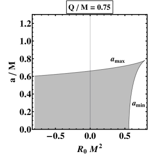
Figure 2: The shaded regions, delimited by the upper $a_{max}$ and lower $a_{min}$ curves, represent the values of $a/M$ for which the existence of BH is possible once $R_{0}\,M^{2}$ value is fixed. It is shown for $Q\,/\,M=0$ and $Q\,/\,M=0.75$ on the left and right panels repectively. Note that $R_{0}$ has dimensions of [length]^-2 when normalizing.

it is remarkable that, from a certain positive value of the curvature $R_{0}^{\,crit}$ onward, the $h$ factor goes to zero for two values of $a$, i.e., apart from the usual $a_{max}$ for which the BH turns $extremal$, there is now a spin lower bound $a_{min}$, below which the BH turns into a marginal extremal BH, as we discussed before. Therefore

$$h\,(a_{max},\,M,\,|R_{0}|\geq 0,\,Q)=0\,\,\,\,\,\,$$

$$\Rightarrow\,\,a_{max}\equiv a_{max}\,(M,\,|R_{0}|\geq 0,\,Q)\,,$$ (22)

$$h\,(a_{min},\,M,\,R_{0}\geq R_{0}^{\,crit}>0,\,Q)=0\,\,\,\,\,\,$$

$$\Rightarrow\,\,a_{min}\equiv a_{min}\,(M,\,R_{0}\geq R_{0}^{\,crit}>0,\,Q)\,.$$ (23)

Due to the excessive length of the equations that describe the behavior of $a_{max}$ and $a_{min}$, we prefer not to display them here. Instead, in Figure 2 we show –for certain values of the electric charge $Q$ parameter $Q$ – the range of values of the spin $a$ parameter for which BH are allowed taking into account. To do so, the corresponding $R_{0}$ value is determined by the parameters defining each $f(R)$ model, as can be seen from equation (8).

III.3 Stationary Limit Surfaces

Another interesting feature of Kerr-Newman BH are Stationary Limit Surfaces (SLS), given by $g_{tt}=0$. For Boyer-Lindquist coordinates, this condition translates into:

$$\frac{\Delta_{\theta}\,\sin^{2}{\theta}\,a^{2}}{\rho^{2}\,\Xi^{2}}-\frac{\Delta_{r}}{\rho^{2}\,\Xi^{2}}=0,$$ (24)

that leads to the fourth order equation

$$r^{4}+\left(a^{2}-\frac{12}{R_{0}}\right)\,r^{2}+\frac{24\,M}{R_{0}}\,r-\left(a^{2}\,\cos^{2}{\theta}+\frac{12}{R_{0}}\right)\,a^{2}\,\sin^{2}{\theta}-\frac{12}{R_{0}}\,(a^{2}+Q^{2})=\,0,$$ (25)

which can be rewritten as:

$$(r-r_{S\,-})(r-r_{S\,int})(r-r_{S\,ext})(r-r_{S\,cosm})=0.$$ (26)

From this equation it follows that each horizon has one ”associated” SLS. Both hypersurfaces coincide at $\theta=0,\pi$ as seen when comparing (25) with equation (19). A complete scheme of BH horizons and SLS structure is shown in Figure 3 for both signs of $R_{0}$.

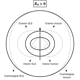
Figure 3: On the left: diagram of a Kerr-Newman BH structure with negative curvature solution $R_{0}=-0.4<0$, $M=1$, $a=0.85$ and $Q=0.35$ ($h>0$). Right: BH structure with positive curvature solution $R_{0}=0.4>0$, $M=1$, $a=0.9$ and $Q=0.4$ ($h<0$). Dotted surfaces represent the SLS whereas horizons are shown with continuous lines. The rotation axis of the BH is indicated by the vertical arrow. In both types of BH, the region between the exterior SLS $r_{S\,ext}$ and its associated exterior horizon $r_{ext}$ is known as ergoregion.

IV Black Hole Thermodynamics

From now on, we will focus our study on BH with a well-defined horizon structure and only for $R_{0}$ negative values of. This last choice is motivated by the problems arising when normalizing the temporal Killing $\xi\equiv\partial_{t}$ in positive curvature spacetimes. This problem is more extensively examined in Cosmohorizon . $R_{0}<0$ choice will allow us to define the thermodynamical quantities of the BH. The rotation Killing field $\psi\equiv\partial_{\phi}$ is uniquely determined by the condition that their orbits should be closed curves with a length parameter equal to $2\pi$. Nevertheless, there is not an adequate criterion to normalize the Killing vector $\xi\equiv\partial_{t}$ in the $dS$ ($R_{0}>0$) Universe since multiplicative constants can be added to $\xi$ and the obtained Killing vectors continue being null on the horizon. In the $AdS$ ($R_{0}<0$), the normalization is done without problems by imposing that the $\xi$ value tends to $\,r\left(-12\,/\,R_{0}\right)^{1/2}$ as $r$ goes to infinity.

In order to study the different thermodynamical properties of Kerr-Newman BH in $f(R)$ theories, we start looking for the temperature of the exterior horizon $r_{ext}\equiv r_{ext}\left(R_{0},\,a,\,Q,\,M\right)$. For that purpose, we will use the Euclidean action method HGG . Performing the change $t\rightarrow-i\tau$, $a\rightarrow ia$ on the metric (12) we obtain the Euclidean section, whose non singular metric is positive-definite, and time coordinate has now angular character around the “axis” $r=r_{ext}$. Regularity of the metric at $r=r_{ext}$ requires the identification of points:

$$(\tau,\,r,\,\theta,\,\phi)\,\sim\,(\tau+i\,\beta,\,r,\,\theta,\,\phi+i\,\beta\,\Omega_{H}),$$ (27)

where $\beta$, which represents the period of the imaginary time on the Euclidean section, it’s the inverse Hawking temperature:

$$\beta=\frac{\displaystyle 4\pi\left(r_{ext}^{2}+a^{2}\right)}{\displaystyle r_{ext}\left[1-\frac{R_{0}\,a^{2}}{12}-\frac{R_{0}\,r_{ext}^{2}}{4}-\frac{\left(a^{2}+Q^{2}\right)}{r_{ext}^{2}}\right]}\equiv\frac{1}{T_{E}},$$

(28)

and $\Omega_{H}$ is the angular velocity of the rotating horizon, which is the same for all the horizon:

$$\Omega_{H}=\frac{a\,\Xi}{\displaystyle r_{ext}^{2}+a^{2}}.$$ (29)

Considering that the event horizon is also a Killing horizon of the Killing vector $\chi=\xi+\Omega_{H}\psi$ (where, as was said before, $\xi\equiv\partial_{t}$ and $\psi\equiv\partial_{\phi}$ are the vectors that asymptotically represent time translations and rotations respectively), $\Omega_{H}$ could be also obtained demanding $\chi$ to be a null vector on the horizon:

$$\left.\chi^{\mu}\chi_{\mu}\right|_{r=r_{ext}}=0$$ (30)

BH horizon temperature could have also been obtained through Killing vectors, as is explained in Hawking1974 where temperature is defined as follows:

$$T_{\kappa}\equiv\frac{\kappa}{4\,\pi},$$ (31)

with $\kappa$ the surface gravity defined by:

$$\chi^{\mu}\,\nabla_{\mu}\chi_{\nu}=\kappa\,\chi_{\nu}.$$ (32)

It can be verified that $\kappa$ is the same at any horizon point and consequently $T_{\kappa}=T_{E}$ as obtained in Bardeen1973 .

Now that we know the expression for the temperature, we consider the Euclidean action in order to obtain the remaining thermodynamical quantities:

$$\Delta S_{E}=\frac{1}{16\pi}\int_{\cal Y}\text{d}^{4}x\sqrt{\mid g\mid}\,\left(R_{0}+f(R_{0})-F_{\mu\nu}F^{\mu\nu}\right)\,,$$

with ${\cal Y}$ the integration region. As is described in Hawking&Page , one has to calculate the difference in four-volumes of the two metrics, identified by the same imaginary time. Provided that the metric is stationary, integration over time simply leads to a multiplicative factor $\beta$. On the other hand, keeping in mind that Maxwell’s equations $\nabla_{\nu}F^{\mu\nu}=0$ must be satisfied, we can rewrite the third term in the integrand as a divergence:

$$F_{\mu\nu}F^{\mu\nu}=\nabla_{\nu}(2\,F^{\mu\nu}\,A_{\mu}),$$ (34)

and therefore:

$$\Delta S_{E}=\frac{R_{0}+f(R_{0})}{16\,\pi}\,\beta\,\Delta\mbox{V}+\frac{1}{8\pi}\int_{\cal{\partial Y}}F^{\mu\nu}\,A_{\mu}\,\text{d}\Sigma_{\nu}\,,$$

where $\partial\cal{Y}=$ $S^{1}\times S^{2}$ is the boundary of the considered region, $S^{2}$ is a 2-sphere whose radius has to be sent to infinity after the integration, and $\Delta\mbox{V}$ is the volume difference between both solutions (corresponding to the black hole metric and that of $AdS$ space identified with the same imaginary time). After some calculation, we obtain:

$$\Delta S_{E}=\frac{\beta\,\left(R_{0}+f(R_{0})\right)}{24\,\Xi}\left[r_{ext}^{3}+\left(a^{2}+\frac{12}{R_{0}}\right)\,r_{ext}+\frac{12\,a^{2}}{R_{0}\,r_{ext}}\right]+\frac{\beta}{2}\,\Phi_{e}\,{\cal{Q}}\,\left(\frac{r_{ext}^{2}+a^{2}}{2\,r_{ext}^{2}}+1\right),$$ (36)

where $\Phi_{e}$ is the electric potential of the horizon as seen from infinity:

$$\Phi_{e}=\left.A_{\mu}\chi^{\mu}\right|_{r\rightarrow\infty}-\left.A_{\mu}\chi^{\mu}\right|_{r=r_{ext}}=\frac{q\,r_{ext}}{r_{ext}^{2}+a^{2}}\,,$$ (37)

and ${\cal{Q}}$ is the physical electric charge of the BH, obtained integrating the flux of the electromagnetic field tensor at infinity, which happens to be:

$${\cal{Q}}=\frac{q}{\Xi}\,.$$ (38)

We shall remember that these calculations involve the vector potential and the electromagnetic field tensor given in (LABEL:EM), and that’s why the factor $\left(1+f^{\prime}(R_{0})\right)^{-1/2}$ does not appear here. Further analysis of the action reveals that it goes singular for $h=0$, as could be expected from extremal BH, whose temperature $T_{E}=0$ makes the $\beta$ factor diverge. Since thermodynamical potentials are obtained by dividing the action by the $\beta$ factor, they still remain well defined at $T_{E}=0$.

It can also be seen that the action (36) diverges in the limit $a^{2}=-12/R_{0}$, which implies $\Xi=0$. This singular case Footnote1 is further explored in RotationAdS and implies that a 3-dimensional static closed Universe at infinity would rotate with the speed of light. Thus, in order to avoid all these problematic issues, let us assume from now on that:

$$\Xi\,:=\,\left(1+\frac{R_{0}\,a^{2}}{12}\right)>0.$$ (39)

The previous expression will turn out also to be a required condition to ensure a positive area and entropy of the BH, as will be seen below.

By using the expression (36) we can immediately obtain Helmholtz free energy $F$, defined by:

$$F=\frac{\Delta S_{E}}{\beta}+\Omega_{H}\,J,$$ (40)

where the term $\Omega_{H}\,J$ comes from the required Legendre transformation to fix angular momentum, being $J$ the angular momentum of the BH and $\Omega_{H}$ the angular velocity of the horizon computed before in (29). To calculate $J$ we need first the physical mass associated to the BH, which can be calculated from:

$${\cal M}=\frac{\partial\Delta S_{E}}{\partial\beta}=\frac{M}{\Xi}\,\left(1+f^{\prime}(R_{0})\right)\,,$$ (41)

resulting on an angular momentum:

$$J=\frac{a\,{\cal M}}{\Xi}=\frac{a\,M}{\Xi^{2}}\,\left(1+f^{\prime}(R_{0})\right)\,,$$ (42)

where we have used equation (8) on ${\cal M}$ to make the substitution: $2\,(R_{0}+f(R_{0}))\,/\,R_{0}=1+f^{\prime}(R_{0})$. Using again the relation $Q^{2}=q^{2}\,/\,\left(1+f^{\prime}(R_{0})\right)$, and equation (19) to express $M$ as a function of $r_{ext}$, we obtain:

$$F=(1+f^{\prime}(R_{0}))\frac{\displaystyle\left[36\,Q^{2}+12\,r_{ext}^{2}+r_{ext}^{4}\,R_{0}+a^{2}\,(36-r_{ext}^{2}\,R_{0})\right]}{\displaystyle 24\,r_{ext}\,\Xi}\,.$$ (43)

If the condition $1+f^{\prime}(R_{0})>0$ is required to hold in order to obtain positive values of the mass, by analyzing the numerator of $F$, we find $F>0$ for values of the horizon below $r_{ext}^{\,\text{\it limit}}$ (with an associated mass $M^{\,\text{\it limit}}$ through equation (19)), and $F<0$ for larger values.

Using the appropriate thermodynamical relations Caldarelli , we can derive the entropy $S$ of the BH, which reads:

$$S = \beta\,({\cal{M}}-\Omega_{H}\,J)-\Delta S_{E}$$ (44)

$$= (1+f^{\prime}(R_{0}))\,\frac{\pi\,(r_{ext}^{2}+a^{2})}{\displaystyle\Xi}.$$

If we compute now the area ${\cal{A}}_{H}$ of the exterior horizon $r_{ext}$, which can be calculated from the metric (12) doing $r=r_{ext}$ and $t$ constants, we obtain:

$$\text{d}s^{2}_{2}\,=\,\frac{\rho^{2}}{\Delta_{\theta}}\,\text{d}\theta^{2}+\frac{\Delta_{\theta}\,\sin^{2}{\theta}}{\rho^{2}}\,\left[-(r_{ext}^{2}+a^{2})\,\frac{\text{d}\,\phi}{\Xi}\right]^{2}$$ (45)

$${\cal{A}}_{H}\equiv\int\int\sqrt{\text{det\,g}_{(2)}}\,\text{d}\theta\,\text{d}\phi=\frac{4\pi(r_{ext}^{2}+a^{2})}{\Xi}$$ (46)

Therefore one sees straightforwardly that the entropy (44) can be expressed as:

$$S=(1+f^{\prime}(R_{0}))\,\frac{{\cal A}_{H}}{4}\,,$$ (47)

consequently $1+f^{\prime}(R_{0})>0$ is also a mandatory condition to obtain a positive entropy Footnote2 , as we supposed above.

Once the temperature $T$ and the entropy $S$ of the BH are known, we can take a step further and study the heat capacity at constant scalar curvature $R_{0}$ and at fixed spin $a$ and charge $Q$ parameters. From the definition:

$$C=T\left.\frac{\partial S}{\partial T}\right|_{R_{0},a,Q},$$ (48)

we obtain the expression:

$$C=(1+f^{\prime}(R_{0}))\,\frac{\displaystyle 2\pi\,r_{ext}^{2}\,(a^{2}+r_{ext}^{2})\left[a^{2}\,(12+r_{ext}^{2}\,R_{0})+3\,(4\,Q^{2}-4\,r_{ext}^{2}+r_{ext}^{4}\,R_{0})\right]}{\displaystyle\Xi\left[-36\,Q^{2}\,r_{ext}^{2}+a^{4}\,(-12+r_{ext}^{2}\,R_{0})+3\,r_{ext}^{4}\,(4+r_{ext}^{2}\,R_{0})-4a^{2}\,(3\,Q^{2}+12\,r_{ext}^{2}-2\,r_{ext}^{4}\,R_{0})\right]}\,.$$

Provided that the condition (39) holds, it seems interesting to find out for which values of $R_{0}$, $a$, $Q$ and $M$ the denominator of the thermal capacity goes to zero, i.e., the thermal capacity goes through an infinite discontinuity, which corresponds to a BH phase transition. We can distinguish between two kind of BH on this subject depending on the values of the $a$, $Q$ and $M$ parameters and scalar curvature $R_{0}$: $i)$ fast BH, without phase transitions and always positive heat capacity $C>0$. $ii)$ slow BH, presents two phase transitions for two determined values of $r_{ext}$:

$$\left.\frac{\partial T}{\partial r_{ext}}\right|_{R_{0},a,Q}(r_{ext}=r_{ext}^{\textnormal{I}},\,r_{ext}^{\textnormal{II}})\,=\,0,$$ (50)

with $r_{ext}^{\textnormal{I}}<r_{ext}^{\textnormal{II}}$, being $r_{ext}^{\textnormal{I}}$ a local maximum of the temperature $T_{max}$, and $r_{ext}^{\textnormal{II}}$ a local minimum $T_{min}$. BH heat capacity proves to be positive ($C>0$) for $r_{ext}<r_{ext}^{\textnormal{I}}$ and $r_{ext}>r_{ext}^{\textnormal{II}}$, and negative ($C<0$) for $r_{ext}^{\textnormal{I}}<r_{ext}<r_{ext}^{\textnormal{II}}$. Once again two masses $M^{\textnormal{I}}$ and $M^{\textnormal{II}}$ can be associated to the radii $r_{ext}^{\textnormal{I}}$ and $r_{ext}^{\textnormal{II}}$ via equation (19).

In Figure 4 we have visualized the behavior of the temperature $T$, the free energy $F$ and the heat capacity $C$ of a BH for different values of mass $M$, with fixed $a$, $Q$ and $R_{0}$ values . It can also be seen the range of $a$ and $Q$ parameters values that provide slow or fast BH for a constant value of the scalar curvature $R_{0}$.

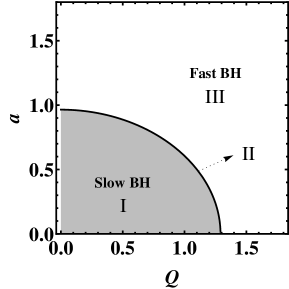
Figure 4: For $R_{0}=-0.2$, we graphically display temperature (up to the left), heat capacity (up to the right), and the free energy (down to the left) of a BH as functions of the mass parameter $M$ for the cases: I) $a=0.5$ y $Q=0$ : “slow” BH that shows a local maximum temperature $T_{max}$ and a local minimum temperature $T_{min}$ at the points where the heat capacity diverges, taking the latter negative values between $T_{max}$ y $T_{min}$. II) $a\approx 0.965$ y $Q=0$ : limit case where $T_{max}$ and $T_{min}$ merge, hence resulting on an inflection point in the temperature and an always positive heat capacity. III) $a=1.5$ y $Q=0$ : “fast” BH with both temperature and heat capacity monotone growing (always positive too). It can be seen that all the configurations acquire a value $F<0$ from a certain value of $M$ onward, given by $r_{ext}^{\,\text{\it limit}}$. The values of $M^{min}$, with $T=0$ and $C=0$, correspond to an extremal BH. Down to the right, for $R_{0}=-0.2$ aswell, we display the regions in which BH behave as “slow” or “fast” BH.

Unlike Schwarzschild-$AdS$ BH case Hawking&Page , Kerr-Newman-$AdS$ BH are allowed for any value of the temperature $T$, hence stability of each BH will be exclusively given by the corresponding values of heat capacity $C$ and free energy $F$ as functions of the $a$, $Q$, $M$ and $R_{0}$ parameters, that ultimately define the BH. However, for a set of fixed values of $a$, $Q$ and $R_{0}$, the mass parameter must be bigger than a minimum $M^{\text{\it min}}$ (characterized by $T=0$) to have BH configuration, otherwise radiation is the only possible equilibrium up to such a minimum mass. For bigger masses, we shall distinguish between the fast and the slow BH. Fast BH, with bigger values of the spin and the electric charge than the slow ones, shows a heat capacity always positive and a positive free energy up to a $M=M^{\,\text{\it limit}}$ value, and negative onwards. Thus, this BH is unstable against tunneling decay into radiation for mass parameter values of $M<M^{\,\text{\it limit}}$. For $M>M^{\,\text{\it limit}}$, free energy becomes negative, therefore smaller than that of pure radiation, that will tend to collapse to the BH configuration in equilibrium with thermal radiation.

The second situation, i.e., the slow BH shows a more complex thermodynamics, being necessary to distinguish between four regions delimited by the mass parameter values: $M^{min}<M^{\textnormal{I}}<M^{\textnormal{II}}<M^{\,\text{\it limit}}$. For $M^{min}<M<M^{\textnormal{I}}$ and for $M^{\textnormal{II}}<M<M^{\,\text{\it limit}}$, both the heat capacity and the free energy are positive, which means that the BH is unstable to decay by tunneling into radiation. If $M^{\textnormal{I}}<M<M^{\textnormal{II}}$, the heat capacity becomes negative but free energy remains positive, being therefore unstable to decay into pure thermal radiation or to larger values of mass. Finally, for $M>M^{\,\text{\it limit}}$ the heat capacity is positive whereas the free energy is now negative, thus tending pure radiation to tunnel to the BH configuration in equilibrium with thermal radiation.

It is mandatory to say that, although not quantitatively, the thermodynamical behavior of these $f(R)$ BH is qualitatively similar to that of GR Caldarelli .

V Particular Examples

In this section we will study some particular $f(R)$ models. For each model we will firstly study the range of parameters that allows the existence of Kerr-Newman BH. Secondly, we will focus on the thermodynamical quantities that define BH stability depending again upon the model range of parameters Footnote3 .

For the sake of simplicity, let us introduce the dimensionless variables:

$$\frac{r}{M}\rightarrow r,\,\,\,\,\frac{a}{M}\rightarrow a,\,\,\,\,\frac{Q}{M}\rightarrow Q,\,\,\,\,R_{0}\,M^{2}\rightarrow R_{0},$$ (51)

where $M$ is the mass parameter, $a$ the spin parameter, $Q$ the electric charge parameter and $R_{0}$ is the scalar curvature obtained as a solution of equation (8). The considered models are:

V.1 Model I: $f(R)\,=\,\alpha|R|^{\beta}$

This model has been widely studied because the $\alpha R^{2}$ term with $\alpha>0$ can account for the accelerated expansion of the Universe. This model can also explain the observed temperature anisotropies observed in the CMB, and could become a viable alternative to scalar field inflationary models; reheating after inflation would have its origin on the production of particles during the oscillation phase of the Ricci scalar Mijic . By using expression (9), we obtain the following scalar curvature solutions:

$$R_{0}^{\pm}=\pm\left[\frac{\pm 1}{(\beta-2)\,\alpha}\right]^{\frac{1}{\beta-1}},$$ (52)

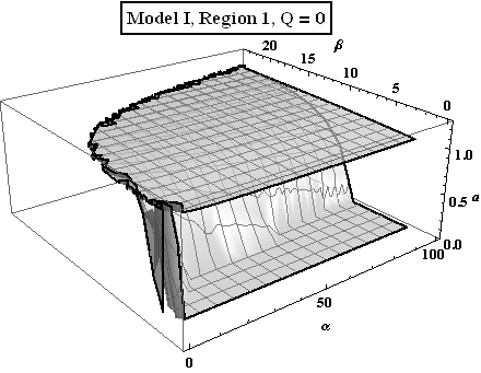
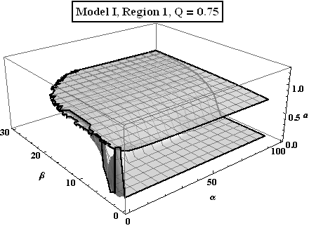
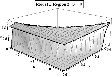
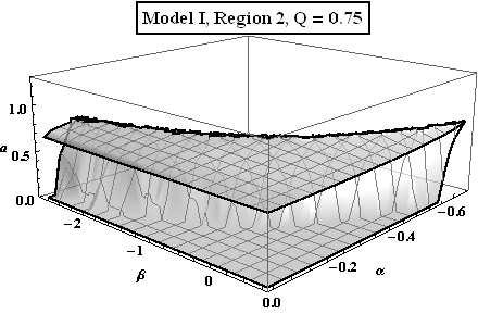
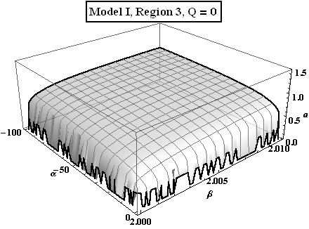
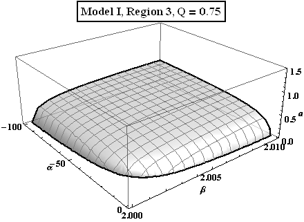
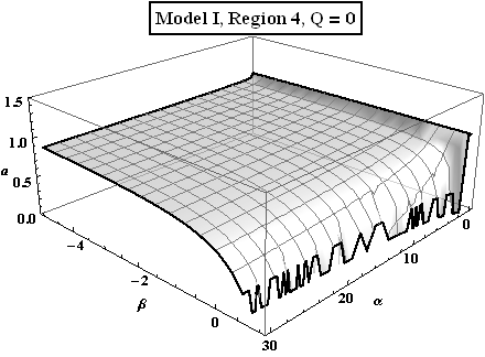
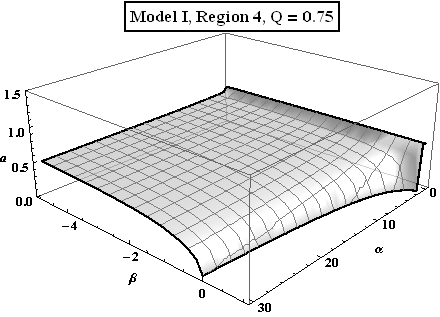
Figure 5: Model I. Region 1: $\left\{\alpha>0,\,\beta>2\right\}$, Region 2: $\left\{\alpha<0,\,\beta<1\right\}$, Region 3: $\left\{\alpha<0,\,\beta>2\right\}$ and Region 4: $\left\{\alpha>0,\,\beta<1\right\}$. BH with a well defined horizon structure will only exist if they have a spin parameter below the upper surface $a_{max}$, and above a second surface $a_{min}$ (in case it exists, Regions 1 and 2 for this model) for certain values of $\alpha$ and $\beta$.

where $R_{0}^{+}$ solution leads to a positive curvature, and $R_{0}^{-}$ to a negative one. The viability condition $1+f^{\prime}(R_{0}^{\pm})>0$ restricts the range of parameters that define this $f(R)$ model to different regions depending on what solution we choose, $R_{0}^{+}$ or $R_{0}^{-}$; for $R_{0}^{+}$ we have Region 1 $\left\{\alpha>0,\,\beta>2\right\}$ and Region 2 $\left\{\alpha<0,\,\beta<1\right\}$, and for $R_{0}^{-}$, Region 3 $\left\{\alpha<0,\,\beta>2\right\}$ and Region 4 $\left\{\alpha>0,\,\beta<1\right\}$. In Figure 5, we show the range of the spin parameter $a$ for which BH are allowed, depending on the parameters $\alpha$ y $\beta$ and for certain values of the charge parameter $Q$. We graphically schematize in Figure 9 the possible thermodynamical configurations as functions of $\alpha$ and $\beta$, for those regions in which $R_{0}<0$.

V.2 Model II: $f(R)\,=\,\pm|R|^{\alpha}\exp{\displaystyle\left(\frac{\beta}{R}\right)}-R$

For this model and by using again expression (9), the scalar curvature, independently of the chosen sign, becomes:

$$R_{0}=\frac{\beta}{\alpha-2}$$ (53)

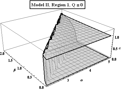
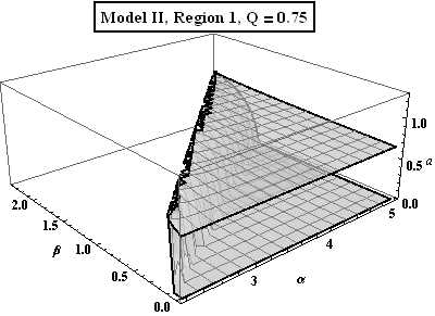
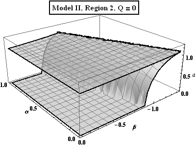
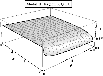
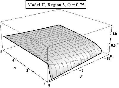
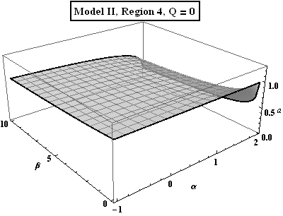
Figure 6: Model II. Región 1: $\left\{\alpha>2,\,\beta>0\right\}$, Region 2: $\left\{\alpha<2,\,\beta<0\right\}$, Region 3: $\left\{\alpha>2,\,\beta<0\right\}$ and Region 4: $\left\{\alpha<2,\,\beta>0\right\}$. BH with a well defined horizon structure will only exist if they have a spin parameter below the upper surface $a_{max}$, and above a second surface $a_{min}$ (in case it exists, Regions 1 and 2 for this model) for certain values of $\alpha$ and $\beta$.

However, the condition $1+f^{\prime}(R_{0})>0$ limits the theory $f(R)$ to different regions depending on what sign we decide to work with. If $R_{0}>0$, the theory is restricted to Region 1 $\left\{\alpha>2,\,\beta>0\right\}$ and Region 2 $\left\{\alpha<2,\,\beta<0\right\}$, for which $R_{0}$ takes positive values. If $R_{0}<0$, we restrict ourselves to Region 3 $\left\{\alpha>2,\,\beta<0\right\}$ and Region 4 $\left\{\alpha<2,\,\beta>0\right\}$. In Figure 6 we show, just as before, the spin parameter $a$ values for which BH can exist in this model depending on the $\alpha$ and $\beta$ parameters defining the model. We graphically schematize in Figure 9 the possible thermodynamical configurations as functions of $\alpha$ and $\beta$, for those regions where $R_{0}<0$.

V.3 Model III: $f(R)\,=\,R\,({\text{Log}}(\alpha\,R))^{\beta}-R$

The associated scalar curvature to this model is:

$$R_{0}=\frac{1}{\alpha}\exp\,({\beta})$$ (54)

In this case the condition $1+f^{\prime}(R_{0})>0$ restricts us to work with Region 1 $\left\{\alpha\in\mathbb{R},\,\beta>0\right\}$, where $R_{0}$ takes positive values for $\alpha>0$ and negatives for $\alpha<0$. In Figure 7 we graphically represent spin parameter $a$ values for which BH present their complete horizon structure, depending on the values of the parameters that define the model. We graphically schematize in Figure 9 the different possible thermodynamical configurations as functions of $\alpha$ and $\beta$, for those regions where $R_{0}<0$.

V.4 Modelo IV: $f(R)\,=\,-\alpha\,\displaystyle\frac{\displaystyle\kappa\left(\frac{R}{\alpha}\right)^{n}}{\displaystyle 1+\beta\left(\frac{R}{\alpha}\right)^{n}}$

This model has been proposed Hu&Sawicki2007 as cosmologically viable. For our study we will consider the case $n=1$, thus having a biparametric theory, as we can define $\gamma=\beta/\alpha$ and then obtain:

$$f(R)\,=\,-\frac{\kappa\,R}{1+\gamma\,R}$$ (55)

Replacing the latter in (9) we obtain two different values for the curvature:

$$R_{0}^{\pm}=-\frac{1-\kappa}{\gamma}\pm\sqrt{\frac{-\kappa\,(1-\kappa)}{\gamma^{2}}},$$ (56)

Keeping in mind that we have to satisfy $1+f^{\prime}(R_{0})>0$, $\kappa$ happens to be restricted to values $\kappa>1$. On the other hand, computation of $1+f^{\prime}(R_{0}^{\pm})$ reveals that $R_{0}^{+}$ is only a valid solution for values of $\kappa$ and $\gamma$ in the Region 1: $\{\kappa>1,\,\gamma>0\}$, and $R_{0}^{-}$ only in Region 2: $\{\kappa>1,\,\gamma<0\}$, being $R_{0}^{+}>0$ and $R_{0}^{-}<0$ in their respective regions. In Figure 8 we show the range of the spin parameter $a$ for which BH are allowed, depending on the parameters $\kappa$ and $\gamma$ for certain values of the charge $Q$. We graphically schematize in Figure 9 the different possible thermodynamical configurations as functions of $\kappa$ and $\gamma$, for those regions in which $R_{0}<0$.

VI Conclusions

In this work we have derived the metric tensor that describes a massive, charged, spinning object for $f(R)$ gravity in metric formalism. We found that it differs from that found by Carter Carter by a multiplicative factor in the electric charge and a redefinition of vacuum scalar curvature.

Further study of the metric allowed us to describe the different astrophysical objects derived from the presence of different horizons: BH, extremal BH, marginal extremal BH, naked singularities and naked extremal singularities. Focusing on BH and their horizon structure, we have seen that these can only exist for values of the spin lower than a maximum value $a_{max}$, and that from a certain positive value of the curvature onward, only above a minimum value $a_{min}$. We have also studied the thermodynamics of $AdS$-like BH (negative curvature solutions) by employing the Euclidean action method. It is observed that some quantities such as the mass, the energy or the entropy of these BH differ from those predicted in GR by a multiplicative factor $1+f^{\prime}(R_{0})$. This factor has to be positive in order to assure a positive mass and entropy for these kind of BH.

On the other hand, analysis of the behavior of the heat capacity of these BH reveals that we can distinguish between two kind of BH: fast and slow, showing the latter two phase transitions. We have also investigated the stability of the different possible configurations that arise from the values of the free energy and the heat capacity, observing that qualitatively the situation is similar to that described by Kerr-Newman-$AdS$ BH. Finally, we considered four $f(R)$ models and analyzed graphically the previous obtained results. Experimental checks to test the validity of a particular $f(R)$ model might be done not only by studying astrophysical BH stability but also if quantum gravity scale is near TeV: since LHC would be producing about one microBH per second microBH , stability and thermodynamical properties of the produced BH might shed some light about the underlying theory of gravity. In this sense, let us remind that the relation between BH mass and temperature in $f(R)$ theories would differ from that predicted by GR.

Acknowledgments: This work has been supported by MICINN (Spain) project numbers FIS 2008-01323, FPA 2008-00592 and Consolider-Ingenio MULTIDARK CSD2009-00064. AdlCD also acknowledges financial support from National Research Foundation (NRF, South Africa) and kind hospitality of UCM, Madrid while elaborating the manuscript.

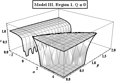
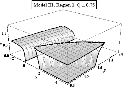
Figure 7: Model III. Region 1: $\left\{\alpha\in\mathbb{R},\,\beta>0\right\}$. BH with a well defined horizon structure will only exist if they have a spin parameter below the upper surface $a_{max}$, and above a second surface $a_{min}$ (that appears in this case for values of $\alpha>0$) for certain values of $\alpha$ and $\beta$.

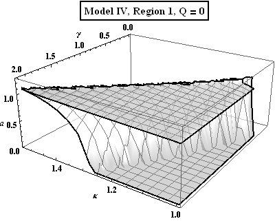
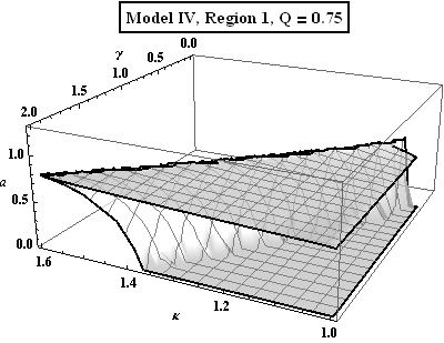
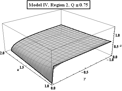
Figure 8: Model IV. Region 1: $\left\{\kappa>1,\,\gamma>0\right\}$ and Region 2: $\left\{\kappa>1,\,\gamma<0\right\}$. BH with a well defined horizon structure will only exist if they have a spin parameter below the upper surface $a_{max}$, and above a second surface $a_{min}$ (in case it exists, only in Region 1 for this model) for certain values of $\kappa$ and $\gamma$.

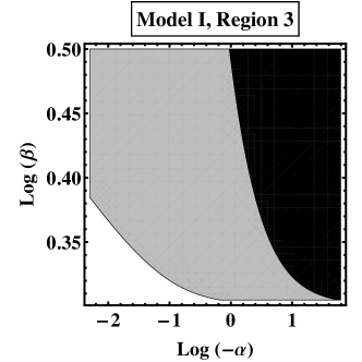
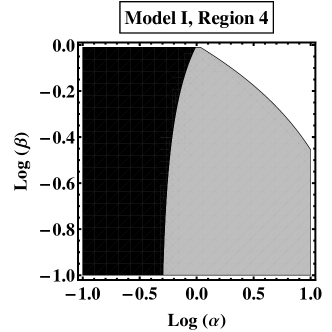
Figure 9: Thermodynamical regions with negative scalar curvature $R_{0}<0$ of the models I, II, III and IV. For the sake of simplicity, we study a BH with the following parameter values: $M=1$, $a=0.4$ and $Q=0.2$. We distinguish between three different regions: i) $C<0$ and $F>0$, in black. ii) $C>0$ and $F>0$, in gray. iii) $C>0$ and $F<0$, in white.

References

- (1) A. G. Riess et al. [Supernova Search Team Collaboration], Astrom. J. 116, 1009 (1998); S. Perlmutter et al. [Supernova Cosmology Project Collaboration], Astrophys. J. 517, 565 (1999); J. L. Tonry et al. Astrophys. J. 594, 1 (2003).
- (2) A. H. Guth, Phys. Rev. Lett. 23, 347-356, (1981).
- (3) P. J. E. Peebles, Principles of Physical Cosmology (1993).
- (4) E. Komatsu et al., Astrophys. J. Suppl. 192, 18 (2011).
- (5) W. J. Percival et al., Mon. Not. Roy. Astron. Soc. 1741 (2009).
- (6) A. G. Riess et al., Astrophys. J. 699, 539 (2009).
- (7) L. Covi, J. E. Kim and L. Roszkowski, Phys. Rev. Lett. 82, 4180 (1999);J. L. Feng, A. Rajaraman and F. Takayama, Phys. Rev. D 68, 085018 (2003); J. L. Feng, A. Rajaraman and F. Takayama, Int. J. Mod. Phys. D 13, 2355 (2004); J. A. R. Cembranos, J. L. Feng, A. Rajaraman and F. Takayama, Phys. Rev. Lett. 95, 181301 (2005); J. A. R. Cembranos, J. L. Feng, L. E. Strigari, Phys. Rev. D 75, 036004 (2007); J. A. R. Cembranos, J. H. Montes de Oca Y., L. Prado, J. Phys. Conf. Ser. 315, 012012 (2011).
- (8) H. Goldberg, Phys. Rev. Lett. 50, 1419 (1983); J. R. Ellis et al., Nucl. Phys. B 238, 453 (1984); K. Griest and M. Kamionkowski, Phys. Rep. 333, 167 (2000); J. A. R. Cembranos, A. Dobado and A. L. Maroto, Phys. Rev. Lett. 90, 241301 (2003); Phys. Rev. D 68, 103505 (2003); AIP Conf.Proc. 670, 235 (2003); Phys. Rev. D 73, 035008 (2006); Phys. Rev. D 73, 057303 (2006); A. L. Maroto, Phys. Rev. D 69, 043509 (2004); Phys. Rev. D 69, 101304 (2004); A. Dobado and A. L. Maroto, Nucl. Phys. B 592, 203 (2001); Int. J. Mod. Phys. D13, 2275 (2004) [hep-ph/0405165]; J. A. R. Cembranos et al., JCAP 0810, 039 (2008).
- (9) J. A. R. Cembranos and L. E. Strigari, Phys. Rev. D 77, 123519 (2008); J. A. R. Cembranos, J. L. Feng and L. E. Strigari, Phys. Rev. Lett. 99, 191301 (2007); J. A. R. Cembranos, A. de la Cruz-Dombriz, A. Dobado, R. Lineros and A. L. Maroto, Phys. Rev. D 83, 083507 (2011).
- (10) J. Alcaraz et al., Phys. Rev.D67, 075010 (2003); P. Achard et al., Phys. Lett. B597, 145 (2004); Europhys. Lett. 82, 21001 (2008); J. A. R. Cembranos, A. Dobado and A. L. Maroto, Phys. Rev. D65 026005 (2002); J. Phys. A 40, 6631 (2007); Phys. Rev. D70, 096001 (2004); J. A. R. Cembranos et al., AIP Conf. Proc. 903, 591 (2007);
- (11) T. Biswas et al., Phys. Rev. Lett. 104, 021601 (2010); JHEP 1010, 048 (2010); Phys. Rev. D 82, 085028 (2010).
- (12) S. Weinberg, Rev. Mod. Phys., 61, 1-23, (1989).
- (13) S. Nojiri and S. D. Odintsov, Phys. Rev. D 68, 123512 (2003); S. Nojiri and S. D. Odintsov, Gen. Rel. Grav. 36,1765 (2004); S. M. Carroll, V. Duvvuri, M. Trodden and M. S. Turner, Phys. Rev. D 70: 043528 (2004); A. Dobado and A. L. Maroto Phys. Rev. D 52, 1895 (1995); G. Dvali, G. Gabadadze and M. Porrati, Phys. Lett. B 485, 208 (2000); J. A. R. Cembranos, Phys. Rev. Lett. 102, 141301 (2009); AIP Conf. Proc. 1182, 288 (2009); J. Phys. Conf. Ser. 315, 012004 (2011); Phys. Rev. D 73, 064029 (2006); J. A. R. Cembranos, K. A. Olive, M. Peloso and J. P. Uzan, JCAP 0907, 025 (2009); S. Nojiri and S. D. Odintsov, Int. J. Geom. Meth. Mod. Phys. 4 115, (2007); J. Beltrán and A. L. Maroto, Phys. Rev. D 78, 063005 (2008); JCAP 0903, 016 (2009); Phys. Rev. D 80, 063512 (2009); Int. J. Mod. Phys. D 18, 2243-2248 (2009).
- (14) S. Nojiri and D. Odintsov, Phys. Rept. 505, 59-144 (2011).
- (15) A. De Felice and S. Tsujikawa, Living Rev. Rel. 13, 3 (2010); S. Capozziello and M. De Laurentis, [gr-qc/1108.6266].
- (16) T. P. Sotiriou, Gen. Rel. Grav. 38 1407, (2006); V. Faraoni, Phys. Rev. D 74 023529, (2006); S. Nojiri and S. D. Odintsov, Phys. Rev. D 74 086005, (2006); I. Sawicki and W. Hu, Phys. Rev. D 75 127502, (2007).
- (17) A. de la Cruz-Dombriz and A. Dobado, Phys. Rev. D 74 087501, (2006); Shin’ichi Nojiri and Sergei D. Odintsov, Phys. Rept. 505, 59-144 (2011); Peter K. S. Dunsby, Emilio Elizalde, Rituparno Goswami, Sergei Odintsov and Diego Sáez-Gómez, arXiv:1005.2205v3 [gr-qc].
- (18) A. de la Cruz-Dombriz, A. Dobado and A. L. Maroto, Phys. Rev. D 77 123515 (2008)
- (19) A. de la Cruz-Dombriz, A. Dobado and A. L. Maroto, Phys. Rev. Lett. D 103, 179001 (2009).
- (20) M. Cvetic, S. Nojiri and S. D. Odintsov, Nucl. Phys. B 628, 295 (2002).
- (21) R. G. Cai, Phys. Rev. D 65, 084014 (2002).
- (22) Y. M. Cho and I. P. Neupane, Phys. Rev. D 66, 024044 (2002).
- (23) R. G. Cai, Phys. Lett. B 582, 237 (2004); J. Matyjasek, M. Telecka and D. Tryniecki, Phys. Rev. D 73, 124016 (2006).
- (24) Mu-in Park, JHEP 0909, 123 (2009); H. W. Lee, Y.-W. Kim and Y. S. Myung, Eur. Phys. J. C68, 255-263, (2010); A. Castillo and A. Larranaga, Electron. J. Theor. Phys. 8 1-10, (2011).
- (25) S. Mignemi and D. L. Wiltshire, Phys. Rev. D 46, 1475 (1992).
- (26) T. Multamaki and I. Vilja, Phys. Rev. D 74, 064022 (2006).
- (27) G. J. Olmo, Phys. Rev. D 75, 023511 (2007).
- (28) A. M. Nzioki, S. Carloni, R. Goswami and P. K. S. Dunsby, Phys. Rev. D81 084028 (2010).
- (29) T. Moon et al. [arXiv:gr-qc/1101.1153v2].
- (30) S. Capozziello, M. De Laurentis and A. Stabile, Class. Quant. Grav. 27, 165008 (2010).
- (31) Y. S. Myung, Phys. Rev. D84 024048 (2011).
- (32) D. N. Vollick, Phys. Rev. D 76, 124001 (2007).
- (33) G. Cognola, E. Elizalde, S. Nojiri, S. D. Odintsov and S. Zerbini, JCAP 0502, 010 (2005).
- (34) S. W. Hawking and D. N. Page, Commun. Math. Phys. 87 577 (1983).
- (35) E. Witten, Adv. Theor. Math. Phys. 2, 505 (1998).
- (36) F. Briscese and E. Elizalde, Phys. Rev. D 77, 044009 (2008).
- (37) A. de la Cruz-Dombriz, A. Dobado and A. L. Maroto, Phys. Rev. D 80, 124011 (2009) [Erratum: Phys. Rev. D 83, 029903(E) (2011)].
- (38) L. Pogosian and A. Silvestri, Phys. Rev. D 77, 023503 (2008).
- (39) V. Faraoni, Phys. Rev. D 75, 067302 (2007).
- (40) A. Nunez and S. Solganik, [arXiv:hep-th/0403159].
- (41) W. Hu and I. Sawicki, Phys. Rev. D 76 064004, (2007).
- (42) B. Carter in Les Astres Occlus ed. by C. M. DeWitt, (Gordon and Breach, New York) (1973).
- (43) Roy. P. Kerr, Phys. Rev. Lett. D 11, 237–238 (1963).
- (44) Ludovico Ferrari, Ars Magna (1545).
- (45) G. W. Gibbons and S. W. Hawking, Phys. Rev. D 15, 2738 (1977).
- (46) G. W. Gibbons and S.W. Hawking, Phys. Rev. D 15, 2752 (1977).
- (47) S. W. Hawking, Commun. Math. Phys. 43 199 (1975) [Erratum-ibid. 46 206 (1976)].
- (48) J. M. Bardeen, B. Carter and S. W. Hawking, Commun. Math. Phys. 31 161 (1973).
- (49) Note that the metric (12) would be singular at .
- (50) S. W. Hawking, C. J. Hunter and M. M. Taylor-Robinson, Phys. Rev. D 59 064005 (1999).
- (51) If for example we want to recover GR with a cosmological constant taking , this relation turns into: , i.e. the famous Bekenstein result Bekenstein .
- (52) M. M. Caldarelli, G. Cognola and D. Klemm, Class. Quant. Grav. 17 399-420 (2000).
- (53) J. D. Bekenstein, Phys. Rev. D 7, 2333 (1973).
- (54) Let us remind at this stage that thermodynamical analysis is restricted to condition as explained in the beginning of Section IV.
- (55) M. B. Mijíc, M. S. Morris and W. M. Suen, Phys. Rev. D 34 2934-2946 (1986).
- (56) W. Hu and I. Sawicki, Phys. Rev. D 76 064004 (2007).
- (57) S. Dimopoulos and G. L. Landsberg, Phys. Rev. Lett. 87 161602 (2001); G. L. Alberghi, R. Casadio and A. Tronconi, J. Phys. G 34 767-778 (2007).