Additive-State-Decomposition-Based Output Feedback Tracking Control for Systems with Measurable Nonlinearities and Unknown Disturbances

Quan Quan, Kai-Yuan Cai, Hai Lin Quan Quan is with Department of Automatic Control, Beihang University, Beijing, 100191, China, was with Department of Electrical and Computer Engineering, National University of Singapore, Singapore, 117576, Singapore. Email: (see http://quanquan.buaa.edu.cn).Kai-Yuan Cai is with Department of Automatic Control, Beihang University, Beijing, 100191, China.Hai Lin is with Department of Electrical and Computer Engineering, National University of Singapore, Singapore, 117576, Singapore.
Abstract

In this paper, a new control scheme, called additive-state-decomposition-based tracking control, is proposed to solve the output feedback tracking problem for a class of systems with measurable nonlinearities and unknown disturbances. By the additive state decomposition, the output feedback tracking task for the considered nonlinear system is decomposed into three independent subtasks: a pure tracking subtask for a linear time invariant (LTI) system, a pure rejection subtask for another LTI system and a stabilization subtask for a nonlinear system. By benefiting from the decomposition, the proposed additive-state-decomposition-based tracking control scheme i) can give a potential way to avoid conflict among tracking performance, rejection performance and robustness, and ii) can mix both designs in time domain and frequency domain for one controller design. To demonstrate the effectiveness, the output feedback tracking problem for a single-link robot arm subject to a sinusoidal or a general disturbance is solved respectively, where the transfer function method for tracking and rejection and the feedback linearization method for stabilization are applied together to the design.

Index Terms:
Additive state decomposition, output feedback, measurable nonlinearities, tracking, rejection.

I Introduction

In this paper, the output feedback tracking problem for a class of systems with measurable nonlinearities and unknown disturbances is considered. This problem has attracted great research interest in recent years [1]-[7]. As far as nonlinear systems are concerned, several results are available under the minimum phase assumption. In [1], global disturbance rejection with stabilization for nonlinear systems in output feedback form was solved in spite of the disturbance generated by a finite dimensional exosystem. The similar problem but subject to unknown parameters on both input matrix and system matrix was considered in [2]. In [7], another control algorithm in simplicity of implementation was proposed for nonlinear plants with parametric and functional uncertainty in the presence of biased harmonic disturbance. The problem about nonminimum phase nonlinear systems was further considered. In [3]-[4], adaptive estimation of unknown disturbances in a class of nonminimum phase nonlinear systems, and the stabilization and disturbance rejection based on the estimated disturbances for single-input single-output (SISO) systems were solved. The result was further extended to a class of nonminimum phase nonlinear Multiple-Input Multiple-Output (MIMO) systems in [5]. In [6], a solution to this problem was provided for nonminimum phase systems with uncertainties in both parameters and order of an exosystem.

The basic idea of the current work is to decompose the output feedback tracking task into simpler subtasks. Then one can design a controller for each subtask respectively, which are finally integrated together to achieve the original control task. The motivation of this paper can be described as follows. First, it is to avoid conflict among tracking performance, rejection performance and robustness. It is well known that there is an intrinsic conflict between performance (trajectory tracking and disturbance rejection) and robustness in the standard feedback framework [8],[9]. By the control scheme mentioned in [1]-[7], as the dimension of the exosystem is increasing, the closed-loop system will be incorporated into a copy of marginally stable exosystem according to internal model principle [10] to achieve high performance (trajectory tracking and disturbance rejection). The price to be paid is a reduced robustness against uncertainties, especially for nonminimum phase systems. Moreover, conflict between tracking performance and rejection performance exists as well when reference and disturbance behave differently [11]. Secondly, it is to relax the restriction on the disturbance. For the control scheme mentioned in [1]-[6], a “regulator equation” often needs to be solved first for a coordinate transformation, which yields an error system with disturbances appearing at the input. However, these control schemes are only applicable to finite-dimensional autonomous exosystems. While, the control scheme mentioned in [7] requires the system being minimum phase to shift disturbances to the input channel.

For such a purpose, a new control scheme based on the additive state decomposition111In this paper we have replaced the term “additive decomposition” in [12] with the more descriptive term “additive state decomposition”., called additive-state-decomposition-based tracking control, is proposed which is applicable to both minimum phase and nonminimum phase systems. The proposed additive state decomposition is a new decomposition manner different from the lower-order subsystem decomposition methods existing in the literature, see e.g. [13],[14]. Concretely, taking the system $\dot{x}\left(t\right)=f\left(t,x\right),x\in\mathbb{R}^{n}$ for example, it is decomposed into two subsystems: $\dot{x}_{1}\left(t\right)=f_{1}\left(t,x_{1},x_{2}\right)$ and $\dot{x}_{2}\left(t\right)=f_{2}\left(t,x_{1},x_{2}\right)$, where $x_{1}\in\mathbb{R}^{n_{1}}$ and$\ x_{2}\in\mathbb{R}^{n_{2}},$ respectively. The lower-order subsystem decomposition satisfies

$$n=n_{1}+n_{2}\text{ and }x=x_{1}\oplus x_{2}.$$

By contrast, the proposed additive state decomposition satisfies

$$n=n_{1}=n_{2}\text{ and}\ x=x_{1}+x_{2}.$$

In our opinion, lower-order subsystem decomposition aims to reduce the complexity of the system itself, while the additive state decomposition emphasizes the reduction of the complexity of tasks for the system.

By following the philosophy above, in the additive-state-decomposition-based tracking control scheme, the output feedback tracking is ‘additively’ decomposed into three independent subtasks, namely the tracking subtask, the rejection subtask and the stabilization subtask. Three subcontrollers for the three subtasks are designed separately then. Since the resulting controller possesses three degrees of freedom, the proposed scheme in fact gives a potential way to avoid conflict among tracking performance, rejection performance and robustness. Moreover, by the additive-state-decomposition-based tracking control scheme, it will be seen that both the tracking subtask and rejection subtask only need to be achieved on a linear time invariant (LTI) system. Consequently, the tracking controller and disturbance compensator can be designed in both time domain and frequency domain. In this framework, the existing output regulation methods as in [1]-[6] can be incorporated. Also, it can take advantage of some standard design methods in frequency domain to handle general disturbances. More importantly, nonminimum phase systems can be handled in the same framework.

This paper is organized as follows. In Section 2, the problem formulation is given and the additive state decomposition is recalled briefly first. In Section 3, the considered system is transformed to a disturbance-free system in sense of input-output equivalence. Sequently, in Section 4, the transformed system is ‘additively’ decomposed into three subsystems. In Section 5, controller design is given. Section 6 concludes this paper.

II Problem Formulation and Additive Decomposition

II-A Problem Formulation

Consider a class of SISO nonlinear systems similar to [1]-[4],[6]-[7]:

$\displaystyle\dot{x}$ $\displaystyle=A_{0}x+bu+\phi_{0}\left(y\right)+d,x\left(0\right)=x_{0}$
$\displaystyle y$ $\displaystyle=c^{T}x$ (1)

where $A_{0}\in\mathbb{R}^{n\times n}$ is a constant matrix, $b\in\mathbb{R}^{n}$ and $c\in\mathbb{R}^{n}$ are constant vectors, $\phi_{0}:\mathbb{R}\rightarrow\mathbb{R}^{n}$ is a nonlinear function vector, $x\left(t\right)\in\mathbb{R}^{n}$ is the state vector, $y\left(t\right)\in\mathbb{R}$ is the output, $u\left(t\right)\in\mathbb{R}$ is the control, and $d\left(t\right)\in\mathbb{R}^{n}$ is a bounded disturbance. It is assumed that only $y$ is available from measurement. The desired trajectory $r\left(t\right)\in\mathbb{R}$ is known and smooth enough, $t\geq 0$. In the following, for convenience, we will omit the variable $t$ except when necessary.

Remark 1. Under certain conditions, the system in the form

$\displaystyle\dot{x}$ $\displaystyle=f\left(x\right)+g\left(x\right)u+d$
$\displaystyle y$ $\displaystyle=h\left(x\right)$

can be transformed to (1). The sufficient and necessary condition to ensure the existence of transformation can be found in [15].

Remark 2. The considered SISO nonlinear system (1) is allowed to be a nonminimum phase system, i.e., the transfer function of the linear part (i.e., regardless of nonlinear dynamics $\phi_{0}\left(y\right)$ and disturbance $d$)

$$c^{T}\left(sI-A_{0}\right)^{-1}b=\frac{N\left(s\right)}{D\left(s\right)}$$

is nonminimum phase here, where $N\left(s\right)$ has zeros on the right $s$-plane. It is noticed that the property of nonminimum phase cannot be changed by output feedback.

For system (1), the following assumption is made.

Assumption 1. The pair $\left(A_{0},c\right)$ is observable.

Under Assumption 1, the objective here is to design a tracking controller $u$ such that $y\rightarrow r$ as $t\rightarrow\infty$ or with good tracking accuracy, i.e, $y-r$ is ultimately bounded by a small value.

II-B Additive State Decomposition

In order to make the paper self-contained, additive state decomposition [12] is recalled here briefly. Consider the following ‘original’ system:

$$f\left({t,\dot{x},x}\right)=0,x\left(0\right)=x_{0}$$ (2)

where $x\in\mathbb{R}^{n}$. We first bring in a ‘primary’ system having the same dimension as (2), according to:

$$f_{p}\left({t,\dot{x}_{p},x_{p}}\right)=0,x{{}_{p}}\left(0\right)=x_{p,0}$$ (3)

where ${x_{p}}\in\mathbb{R}^{n}$. From the original system (2) and the primary system (3) we derive the following ‘secondary’ system:

$$f\left({t,\dot{x},x}\right)-f_{p}\left({t,\dot{x}_{p},x_{p}}\right)=0,x\left(0\right)=x_{0}$$ (4)

where ${x_{p}}\in\mathbb{R}^{n}$ is given by the primary system (3). Define a new variable ${x_{s}}\in\mathbb{R}^{n}$ as follows:

$${x_{s}\triangleq x-x_{p}}.$$ (5)

Then the secondary system (4) can be further written as follows:

$$f\left({t,\dot{x}_{s}+\dot{x}_{p},x_{s}+x_{p}}\right)-f_{p}\left({t,\dot{x}_{p},x_{p}}\right)=0,x{{}_{s}}\left(0\right)=x_{0}-x_{p,0}.$$ (6)

From the definition (5), we have

$${x}\left(t\right)={x_{p}\left(t\right)+x_{s}\left(t\right),t\geq 0.}$$ (7)

Remark 3. By the additive state decomposition, the system (2) is decomposed into two subsystems with the same dimension as the original system. In this sense our decomposition is “additive”. In addition, this decomposition is with respect to state. So, we call it “additive state decomposition”.

As a special case of (2), a class of differential dynamic systems is considered as follows:

$\displaystyle\dot{x}$ $\displaystyle=f\left({t,x}\right),x\left(0\right)=x_{0},$
$\displaystyle y$ $\displaystyle=h\left({t,x}\right)$ (8)

where ${x}\in\mathbb{R}^{n}$ and $y\in\mathbb{R}^{m}.$ Two systems, denoted by the primary system and (derived) secondary system respectively, are defined as follows:

$\displaystyle\dot{x}_{p}$ $\displaystyle=f_{p}\left({t,x_{p}}\right),x_{p}\left(0\right)=x_{p,0}$
$\displaystyle y_{p}$ $\displaystyle=h_{p}\left({t,x}_{p}\right)$ (9)

and

$\displaystyle\dot{x}_{s}$ $\displaystyle=f\left({t,x_{p}}+{x_{s}}\right)-f_{p}\left({t,x_{p}}\right),x_{s}\left(0\right)=x_{0}-x_{p,0},$
$\displaystyle y_{s}$ $\displaystyle=h\left({t,x_{p}}+{x_{s}}\right)-h_{p}\left({t,x}_{p}\right)$ (10)

where ${x_{s}}\triangleq{x-x_{p}}$ and $y_{s}\triangleq{y-y_{p}}$. The secondary system (10) is determined by the original system (8) and the primary system (9). From the definition, we have

$${x}\left(t\right)={x_{p}\left(t\right)+x_{s}\left(t\right),y\left(t\right)=y_{p}\left(t\right)+y_{s}\left(t\right),t\geq 0.}$$ (11)

III Model Transformation

Firstly, we need to estimate the state from the output. The main difficulty is how to handle the disturbances in the state equation. In [1]-[7], an extended state observer including states of the considered nonlinear system and the exosystem is designed, where the disturbance is assumed to be generated by a finite-dimensional autonomous exosystem. According to this, the model of the disturbance has in fact determined the performance of the observation partly. However, in practice, a general disturbance is difficult to model as a finite-dimensional autonomous one, or with uncertainties. To tackle this difficulty, we first transform the original system (1) to a disturbance-free system, which is proved to be input-output equivalent with the aid of the additive state decomposition as stated in the following theorem.

Theorem 1. Under Assumption 1, there exists a vector $p\in\mathbb{R}^{n}$ such that $A=A_{0}+pc^{T}$ is stable, and the system (1) is input-output equivalent to the following system:

$\displaystyle\dot{x}_{new}$ $\displaystyle=Ax_{new}+bu+\phi\left(y\right),x_{new}\left(0\right)=0$
$\displaystyle y$ $\displaystyle=c^{T}x_{new}+d_{new}$ (12)

where $\phi\left(y\right)=\phi_{0}\left(y\right)-py$ and

$$x_{new}=x-\left(e^{At}x_{0}+\int\nolimits_{0}^{t}e^{A\left(t-s\right)}d\left(s\right)ds\right),d_{new}=c^{T}\left(e^{At}x_{0}+\int\nolimits_{0}^{t}e^{A\left(t-s\right)}d\left(s\right)ds\right).$$ (13)

Proof. Since the pair $\left(A_{0},c\right)$ is observable, there always exists a vector $p\in\mathbb{R}^{n}$ such that $A=A_{0}+pc^{T}$ is stable, whose the eigenvalues can be assigned freely. The system (1) can be rewritten as follows:

$\displaystyle\dot{x}$ $\displaystyle=Ax+bu+\phi\left(y\right)+d,x\left(0\right)=x_{0}$
$\displaystyle y$ $\displaystyle=c^{T}x$ (14)

where $\phi\left(y\right)=\phi_{0}\left(y\right)-py$. In the following, additive state decomposition is utilized to decompose the system (14). Consider the system (14) as the original system and choose the primary system as follows:

$\displaystyle\dot{x}_{p}$ $\displaystyle=Ax_{p}+d,x_{p}\left(0\right)=x_{0}$
$\displaystyle y_{p}$ $\displaystyle=c^{T}x_{p}.$ (15)

Then the secondary system is determined by the original system (14) and the primary system (15) with the rule (10) that

$\displaystyle\dot{x}_{s}$ $\displaystyle=Ax_{s}+bu+\phi\left(y\right),x_{s}\left(0\right)=0$
$\displaystyle y_{s}$ $\displaystyle=c^{T}x_{s}.$ (16)

According to (11), we have $x=x_{p}+x_{s}$ and$\ y=y_{p}+y_{s}.$ Therefore, the following system is an input-output equivalent system of (14):

$\displaystyle\dot{x}_{s}$ $\displaystyle=Ax_{s}+bu+\phi\left(y\right),x_{s}\left(0\right)=0$
$\displaystyle y$ $\displaystyle=c^{T}x_{s}+c^{T}x_{p}$ (17)

where $x_{p}$ is generated by (15). By (15), it holds that $x_{p}=e^{At}x_{0}+\int\nolimits_{0}^{t}e^{A\left(t-s\right)}d\left(s\right)ds.$ Let $x_{s}=x_{new}$ and $d_{new}=c^{T}x_{p}.$ Substituting into (17) yields (12). $\square$

For the disturbance-free transformed system (12), we design an observer to estimate $x_{new}$ and $d_{new}$, which is stated in Theorem 2.

Theorem 2. Under Assumption 1, an observer is designed to estimate state $x_{new}$ and $d_{new}$ in (12) as follows

$\displaystyle\dot{\hat{x}}_{new}$ $\displaystyle=A\hat{x}_{new}+bu+\phi\left(y\right),\hat{x}_{new}\left(0\right)=0$
$\displaystyle\hat{d}_{new}$ $\displaystyle=y-c^{T}\hat{x}_{new}.$ (18)

Then $\hat{x}_{new}\equiv x_{new}$ and $\hat{d}_{new}\equiv d_{new}.$

Proof. Subtracting (18) from (12) results in $\dot{\tilde{x}}_{new}=A\tilde{x}_{new},\tilde{x}_{new}\left(0\right)=0,$ where $\tilde{x}_{new}=x_{new}-\hat{x}_{new}.$ Then $\tilde{x}_{new}\equiv 0$. This implies that $\hat{x}_{new}\equiv x_{new}.$ Consequently, by the relation $y=c^{T}x_{new}+d_{new}$ in (12), we have $\hat{d}_{new}\equiv d_{new}.$ $\square$

Remark 4. By (13), if the new state $x_{new}$ is bounded, then the original state $x$ is bounded as well since the matrix $A$ is stable and the disturbance $d$ is bounded. This explains why the matrix $A$ is chosen to be stable. To eliminate the transient effect of initial values in $d_{new},$ namely $c^{T}e^{At}x_{0},$ we often assign the eigenvalues for $A$ to have large negative real part. By using the new state $x_{new}$, the controller can be designed based on the transformed system (12) directly as shown in the following sections.

Remark 5. It is interesting to note that the new state $x_{new}$ and disturbance $d_{new}$ in the transformed system (12) can be observed directly rather than asymptotically or exponentially. This will facilitate the analysis and design later. In practice, the output $y$ will be more or less subject to noise. In this case, the stable matrix $A$ will result in a small $\tilde{x}_{new}$ in the presence of small noise, i.e. $\hat{x}_{new}$ close to $x_{new}$.

Example 1. A single-link robot arm with a revolute elastic joint rotating in a vertical plane is served as an application in this paper [16]:

$\displaystyle\dot{x}_{1}$ $\displaystyle=x_{2}$
$\displaystyle\dot{x}_{2}$ $\displaystyle=-\frac{F_{l}}{J_{l}}x_{2}-\frac{k}{J_{l}}\left(x_{1}-x_{3}\right)-\frac{Mgl}{J_{l}}\sin x_{1}+d_{1}$
$\displaystyle\dot{x}_{3}$ $\displaystyle=x_{4}$
$\displaystyle\dot{x}_{4}$ $\displaystyle=-\frac{F_{m}}{J_{m}}x_{4}+\frac{k}{J_{m}}\left(x_{1}-x_{3}\right)+\frac{1}{J_{m}}\tau+d_{2}$
$\displaystyle y$ $\displaystyle=x_{1}$ (19)

where $x_{1},x_{2},x_{3},x_{4}$ are the link displacement (rad), link velocity (rad/s), rotor displacement (rad) and rotor velocity (rad/s), respectively; $d_{1}$ and $d_{2}$ are unknown disturbance. The initial value is assumed to be $x\left(0\right)=\left[\begin{array}[c]{cccc}0.05&0&0.05&0\end{array}\right]^{T}.$ Let link inertia $J_{l}=2$kg$\cdot$m${}^{2},$ the motor rotor inertia $J_{m}=0.5$kg$\cdot$m${}^{2},$ the elastic constant $k=0.05$kg$\cdot$m2/s, the link mass $M=0.5$kg, the gravity constant $g=9.8$m/s2, the center of mass $l=0.5$m and viscous friction coefficients $F_{l}=F_{m}=0.2$kg$\cdot$m2/s. The control $\tau$ is the torque delivered by the motor. The control problem here is: assuming only $y$ is measured, $\tau$ is to be designed so that $y$ tracks a smooth enough reference $r$ asymptotically or with good tracking accuracy. The controller $\tau$ in (19) is designed as follows $\tau=J_{m}u,$ where $u$ will be specified later. Then the system (19) can be written in form of (1) with

$$A_{0}=\left[\begin{array}[c]{cccc}0&1&0&0\\ -\frac{k}{J_{l}}&-\frac{F_{l}}{J_{l}}&\frac{k}{J_{l}}&0\\ 0&0&0&1\\ \frac{k}{J_{m}}&0&-\frac{k}{J_{m}}&-\frac{F_{m}}{J_{m}}\end{array}\right],b=\left[\begin{array}[c]{c}0\\ 0\\ 0\\ 1\end{array}\right],c=\left[\begin{array}[c]{c}1\\ 0\\ 0\\ 0\end{array}\right],\phi_{0}\left(y\right)=\left[\begin{array}[c]{c}0\\ -\frac{Mgl}{J_{l}}\sin y\\ 0\\ 0\end{array}\right].$$ (20)

It is easy to verify that the pair $\left(A_{0},c\right)$ is observable. So for this application Assumption 1 holds. It is found that $A_{0}$ is unstable. Choosing $p=\left[\begin{array}[c]{cccc}-2.10&-1.295&-9.36&3.044\end{array}\right]^{T},$ the system (19) is formulated into (12) with

$$A=\left[\begin{array}[c]{cccc}-2.1&1&0&0\\ -1.32&-0.1&0.025&0\\ -9.36&0&0&1\\ 3.144&0&-0.1&-0.4\end{array}\right],\phi\left(y\right)=\left[\begin{array}[c]{c}2.1y\\ 1.295y-1.225\sin y\\ 9.36y\\ -3.044y\end{array}\right].$$

where the eigenvalues of $A$ are assigned as $-0.5,$ $-0.6,$ $-0.7,$ $-0.8.$

IV Additive State Decomposition of Transformed System

In this section, the transformed system (12) is ‘additively’ decomposed into three independent subsystems in charge of corresponding subtasks, namely the tracking subtask, the rejection subtask and the stabilization subtask, as shown in Fig.1. There exist many tools to analyze LTI systems, such as Laplace transformation and transfer function, and state-space techniques. Based on the above consideration, the transformed system (12) is expected to be decomposed into two subsystems by the additive state decomposition: an LTI system including all external signals as the primary system, together with the secondary system free of external signals. Therefore, the original tracking task for the system (12) is correspondingly decomposed into two subtasks by the additive state decomposition: a tracking (including rejection) subtask for an LTI ‘primary’ system and a stabilization subtask for the left ‘secondary’ system. Since the tracking (including rejection) subtask is only assigned to the LTI system, it therefore is a lot easier than that for a nonlinear one. Furthermore, the tracking (including rejection) subtask is decomposed into a pure tracking subtask and a pure rejection subtask.

Refer to caption
Figure 1: Additive state decomposition flow

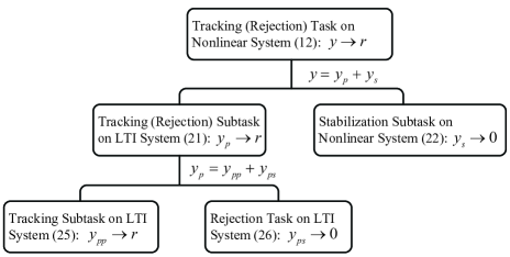
Consider the transformed system (12) as the original system. According to the principle above, we choose the primary system as follows:

$\displaystyle\dot{x}_{p}$ $\displaystyle=Ax_{p}+bu_{p}+\phi\left(r\right)$
$\displaystyle y_{p}$ $\displaystyle=c^{T}x_{p}+d_{new},x_{p}\left(0\right)=0.$ (21)

Then the secondary system is determined by the original system (12) and the primary system (21) with the rule (10), and we can obtain that

$\displaystyle\dot{x}_{s}$ $\displaystyle=Ax_{s}+bu_{s}+\phi\left(r+e_{p}+c^{T}x_{s}\right)-\phi\left(r\right)$
$\displaystyle y_{s}$ $\displaystyle=c^{T}x_{s},x_{s}\left(0\right)=0$ (22)

where $u_{s}=u-u_{p}$ and $e_{p}=y_{p}-r.$ According to (11), we have

$$x_{new}=x_{p}+x_{s}\text{ and }y=y_{p}+y_{s}.$$ (23)

The strategy here is to assign the tracking (including rejection) subtask to the primary system (21) and the stabilization subtask to the secondary system (22). It is clear from (21)-(23) that if the controller $u_{p}$ drives $y_{p}\rightarrow r$ and the controller $u_{s}$ drives $y_{s}\rightarrow 0$ as $t\rightarrow\infty,$ then $y\rightarrow r$ as $t\rightarrow\infty$. The benefit brought by the additive state decomposition is that the controller $u_{s}$ will not affect the tracking and rejection performance since the primary system (21) is independent of the secondary system (22). On the other hand, if the secondary system (22) is input-to-state stable with respect to the signal $e_{p}$, then the dynamics of controller $u_{p}$ will not change the input-to-state stability property. Therefore, conflict between performance (trajectory tracking and disturbance rejection) and robustness is avoided. Since the states $x_{p}$ and $x_{s}$ are unknown except for sum of them, namely $x_{new}$, an observer is proposed to estimate $x_{p}$ and $x_{s}.$

Theorem 3. Under Assumption 1, suppose that an observer is designed to estimate state $x_{p}$ and $x_{s}$ in (21)-(22) as follows:

$\displaystyle\hat{x}_{p}$ $\displaystyle=x_{new}-\hat{x}_{s}$ (24a)
$\displaystyle\dot{\hat{x}}_{s}$ $\displaystyle=A\hat{x}_{s}+bu_{s}+\phi\left(y\right)-\phi\left(r\right),\hat{x}_{s}\left(0\right)=0.$ (24b)
Then $\hat{x}_{p}\equiv x_{p}$ and $\hat{x}_{s}\equiv x_{s}.$

Proof. Subtracting (24b) from (22) results in $\dot{\tilde{x}}_{s}=A\tilde{x}_{s},\tilde{x}_{s}\left(0\right)=0$ 222Since the initial values $x_{new}\left(0\right),x_{s}\left(0\right),\hat{x}_{s}\left(0\right)$ are all assigned by the designer, they are all determinate., where $\tilde{x}_{s}=x_{s}-\hat{x}_{s}.$ Then $\tilde{x}_{s}\equiv 0$. This implies that $\hat{x}_{s}\equiv x_{s}.$ Consequently, by (23), we have $\hat{x}_{p}=x_{new}-\hat{x}_{s}=x_{p}.$ $\square$

To avoid conflict between tracking performance and rejection performance, the tracking subtask for the primary system (21) is further decomposed into two subtasks by the additive state decomposition: a pure tracking subtask and a pure rejection subtask. At this time, consider the primary system (21) as the original system and choose the primary system of (21) as follows:

$\displaystyle\dot{x}_{pp}$ $\displaystyle=Ax_{pp}+bu_{pp}+\phi\left(r\right),$
$\displaystyle y_{pp}$ $\displaystyle=c^{T}x_{pp},x_{pp}\left(0\right)=0.$ (25)

Then the secondary system of (21) is determined by the system (21) and (25) with the rule (10) that

$\displaystyle\dot{x}_{ps}$ $\displaystyle=Ax_{ps}+bu_{ps}$
$\displaystyle y_{ps}$ $\displaystyle=c^{T}x_{ps}+d_{new},x_{ps}\left(0\right)=0,$ (26)

where $u_{ps}=u_{p}-u_{pp}.$ According to (11), we have

$$x_{p}=x_{pp}+x_{ps}\ \text{and}\ y_{p}=y_{pp}+y_{ps}.$$ (27)

It is clear from (25)-(27) that if the controller $u_{pp}$ drives $y_{pp}\rightarrow r$ and the controller $u_{ps}$ drives $y_{ps}\rightarrow 0$ as $t\rightarrow\infty,$ then $y_{p}\rightarrow r$ as $t\rightarrow\infty$. It is noticed that the controller $u_{pp}$ and $u_{ps}$ above are independent each other. So, conflict between tracking performance and rejection performance is avoided.

V Controller Design

So far, we have transformed the original system to a disturbance-free system whose state can be estimated directly. And then, decompose the transformed system into three independent subsystems in charge of corresponding subtasks. In this section, we are going to investigate the controller design with respect to the three decomposed subtasks respectively.

V-A Problem for Tracking Subtask

Problem 1. For (25), design a control input

$\displaystyle\dot{z}^{r}$ $\displaystyle=\alpha^{r}\left(z^{r},x_{pp},r\right)$
$\displaystyle u_{pp}$ $\displaystyle=u^{r}\left(z^{r},x_{pp},r\right)$ (28)

such that $y_{pp}\rightarrow r$ as $t\rightarrow\infty$.

Remark 6 (on Problem 1). Problem 1 can be considered as a stable inversion problem [17],[18], which has been solved for the system in the form of (25) no matter whether it is minimum phase or nonminimum phase. If the system (25) is only minimum phase, then the stable inversion problem is made a lot easier by using the transfer function method. Problem 1 can also be considered as an output regulation problem [1]-[6], if the reference $r$ is generated by an autonomous system. Since the reference $r$ is given, the computation above can be done offline. In addition, since the control design is only for a classical LTI system, the computation is easier compared with that for a nonlinear one.

Example 2 (Example 1 Continued). Since system (19) is minimum phase, by the transfer function method, the reference control input $u_{pp}=u^{r}$ can be designed as follows:

$$u^{r}\left(s\right)=\frac{1}{c^{T}F^{-1}\left(s\right)b}\left[r\left(s\right)+c^{T}F^{-1}\left(s\right)\left(pr\left(s\right)+b_{1}\frac{Mgl}{J_{l}}\left(\sin r\right)\left(s\right)\right)\right]$$ (29)

where $u^{r}\left(s\right)$ is the transfer function of signal $u^{r},$ $F\left(s\right)=sI_{4}-A$ and $b_{1}=\left(\begin{array}[c]{cccc}0&1&0&0\end{array}\right)^{T}$. Then $y_{pp}\rightarrow r$ as $t\rightarrow\infty.$ Problem 1 is solved.

V-B Problem for Rejection Subtask

Problem 2. For (26), there exists a control input

$\displaystyle\dot{z}^{d}$ $\displaystyle=\alpha^{d}\left(z^{d},x_{ps},d_{new}\right)$
$\displaystyle u_{ps}$ $\displaystyle=u^{d}\left(z^{d},x_{ps},d_{new}\right)$ (30)

such that $y_{ps}\rightarrow\mathcal{B}\left(\delta\right)$ 333$\mathcal{B}\left(\delta\right)\triangleq\left\{\xi\in\mathbb{R}\left|\left\|\xi\right\|\leq\delta\right.\right\},$ where $\delta=\delta\left(d\right)$ is a function of the disturbance $d;$ the notation $x\left(t\right)\rightarrow\mathcal{B}\left(\delta\right)$ means $\underset{y\in\mathcal{B}\left(\delta\right)}{\min}$ $\left|x\left(t\right)-y\right|\rightarrow 0.$ as $t\rightarrow\infty$. In particular, if $\delta=0,$ then $y_{ps}\rightarrow 0$ as $t\rightarrow\infty$.

Remark 7 (on Problem 2). Since the system (26) is a classical LTI system, some standard designs in frequency domain, such as the transfer function method, can be used to handle a general disturbance [11]. In this case, the disturbance cannot be often rejected asymptotically. So, the Problem 2 needs to consider the result $y_{ps}\rightarrow\mathcal{B}\left(\delta\right)$ besides $y_{ps}\rightarrow 0.$ If $d_{new}$ is generated by an autonomous system, then Problem 2 can be considered as an output regulation problem [1]-[7]. In this case, the disturbance can be rejected asymptotically. The technique in [1]-[7] of course can be still applied to the problem even if both parameters and order of an exosystem are uncertain.

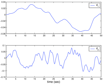
Example 3 (Example 1 Continued). To demonstrate the effectiveness of the proposed control, the disturbances in (19) are assumed to be in two cases. Case 1 (sinusoidal): the unknown disturbances $d_{1}$ and $d_{2}$ are sinusoidal, such as $d_{1}=0.05\sin t$ and $d_{2}=0.05\sin\left(t+1\right).$ Case 2 (general): the unknown disturbances $d_{1}$ and $d_{2}$ are driven by normal $\left(\text{Gaussian}\right)$ distributed random signals $\zeta_{1},\zeta_{2}\sim\mathcal{N}\left(0,1\right).$ The transfer functions are assumed to be $d_{1}\left(s\right)=\frac{0.08}{\left(s+0.2\right)\left(s+0.5\right)\left(s+0.8\right)}\zeta_{1}\left(s\right)$ and $d_{2}\left(s\right)=\frac{6}{\left(s+1\right)\left(s+2\right)\left(s+3\right)}\zeta_{2}\left(s\right)$. The resulting disturbances are shown in Fig.2.

Case 1 (sinusoidal). Since the unknown disturbances $d_{1}$ and $d_{2}$ are sinusoidal with frequency $1$ rad/s, by (13) we can conclude that $d_{new}=\bar{d}+\varepsilon$, where $\bar{d}$ is sinusoidal with frequency $1$ rad/s as well and $\varepsilon\rightarrow 0$ as $t\rightarrow\infty.$ This implies that  the transfer function $\bar{d}$ can be written as $\bar{d}\left(s\right)=\frac{1}{s^{2}+1}w\left(0\right).$ For (26), design controller $u_{ps}=u^{d}$ as follows

$\displaystyle\dot{z}^{d}$ $\displaystyle=Sz^{d}+c_{d}y_{ps}$
$\displaystyle u^{d}$ $\displaystyle=k_{1}^{T}z^{d}+k_{2}^{T}x_{ps}$ (31)

where $S=\left[\begin{array}[c]{cc}0&1\\ -1&0\end{array}\right],$ $c_{d}=\left[\begin{array}[c]{c}1\\ 0\end{array}\right],$ $k_{1}=\left[\begin{array}[c]{cc}96&122\end{array}\right]^{T}$ and $k_{2}=\left[\begin{array}[c]{cccc}34&70&-0.67&-1.9\end{array}\right]^{T}.$ Combining (26) with (31) results in

$\displaystyle\dot{z}^{d}$ $\displaystyle=Sz^{d}+c_{d}c^{T}x_{ps}+c_{d}d_{new}$
$\displaystyle\dot{x}_{ps}$ $\displaystyle=k_{1}^{T}z^{d}+\left(A+bk_{2}^{T}\right)x_{ps}$
$\displaystyle y_{ps}$ $\displaystyle=c^{T}x_{ps}+d_{new}.$

The transfer function from $d_{new}$ to $y_{ps}$ possesses negative real poles and at least two zeros $\pm i.$ Since $\bar{d}\left(s\right)=\frac{1}{s^{2}+1}w\left(0\right)$ and $\varepsilon\rightarrow 0,$ we have $y_{ps}\rightarrow 0.$ Problem 2 is solved for Case 1.

Case 2 (general). The transfer function from $u_{ps}$ to $y_{ps}$ can be represented as follows:

$$y_{ps}\left(s\right)=c^{T}F^{-1}\left(s\right)bu_{ps}\left(s\right)+d_{new}\left(s\right).$$

Since $d_{new}$ is a low-frequency disturbance and can be observed by (18), an easy way is to design the disturbance compensator as follows:

$$u^{d}\left(s\right)=-\frac{1}{c^{T}F^{-1}\left(s\right)b}Q\left(s\right)d_{new}\left(s\right)$$ (32)

where $u^{d}\left(s\right)$ is the transfer function of $u^{d},$ $Q\left(s\right)$ is a low-pass filter satisfying

$$\left(1-Q\left(j\omega\right)\right)d_{new}\left(j\omega\right)\approx 0,\forall\omega\in\mathbb{R}.$$

Moreover, $Q\left(s\right)$ is at least fourth order to make the compensator physically realizable (the order of denominator is greater than or equal to that of numerator). In this simulation, we choose

$$Q\left(s\right)=\frac{1}{\prod\nolimits_{k=5}^{k=8}\left(\frac{1}{10k}s+1\right)}.$$

In this case, $y_{ps}$ in (26) is ultimately bounded by a small value, namely $y_{ps}\rightarrow\mathcal{B}\left(\delta\right)$, where $\delta$ can be adjusted by $Q\left(s\right).$ Problem 2 is solved for Case 2.

V-C Problem for Stabilization Subtask

Problem 3. For (22), there exists a controller $u_{s}=u^{s}\left(x_{s},r,\cdots,r^{\left(N\right)}\right)$ such that the closed-loop system is input-to-state stable with respect to the input $e_{p},$ namely

$$\left\|x_{s}\left(t\right)\right\|\leq\beta\left(\left\|x_{s}\left(t_{0}\right)\right\|,t-t_{0}\right)+\gamma\left(\underset{t_{0}\leq s\leq t}{\sup}\left\|e_{p}\left(s\right)\right\|\right),t\geq t_{0},$$ (33)

where $r^{\left(N\right)}$ denotes the $N$th derivative of $r$, function $\beta$ is a class $\mathcal{KL}$ function and $\gamma$ is a class $\mathcal{K}$ function [19].

Remark 8 (on Problem 3). If $e_{p}$ is nonvanishing, then Problem 3 is a classical input-to-state stability problem. Readers can refer to [19],[20] for how to design a controller satisfying input-to-state stability or how to prove the designed controller satisfying input-to-state stability. In particular, if $e_{p}\rightarrow 0$ as $t\rightarrow\infty,$ then $x_{s}\rightarrow 0$ as $t\rightarrow\infty$ by (33). In addition, if $e_{p}\rightarrow 0$ as $t\rightarrow\infty,$ then input-to-state stability can be relaxed as well. In fact, Problem 3 only considers how $x_{s}$ behaves as $e_{p}\rightarrow 0$ as $t\rightarrow\infty.$ The reference [21] discussed under what conditions the solution of (26) say $x_{s}^{e_{p}}$ and the solution of (26) with $e_{p}\equiv 0$ say $x_{s}^{\ast}$ satisfy $\left\|x_{s}^{e_{p}}\left(t\right)-x_{s}^{\ast}\left(t\right)\right\|\leq\theta e^{-\eta t},$ where $\theta,\eta>0.$ In this case, only stability of (26) with $e_{p}\equiv 0$ needs to be considered rather than input-to-state stability.

Example 4 (Example 1 Continued). The system (22) can be rewritten as

$\displaystyle\dot{x}_{s,1}$ $\displaystyle=x_{s,2}$
$\displaystyle\dot{x}_{s,2}$ $\displaystyle=-\frac{F_{l}}{J_{l}}x_{s,2}-\frac{k}{J_{l}}\left(x_{s,1}-x_{s,3}\right)-\frac{Mgl}{J_{l}}\left[\sin\left(r+x_{s,1}\right)-\sin\left(r\right)\right]+d_{e_{p}}$
$\displaystyle\dot{x}_{s,3}$ $\displaystyle=x_{s,4}$
$\displaystyle\dot{x}_{s,4}$ $\displaystyle=-\frac{F_{m}}{J_{m}}x_{s,4}+\frac{k}{J_{m}}\left(x_{s,1}-x_{s,3}\right)+u_{s}$
$\displaystyle y$ $\displaystyle=x_{s,1}$ (34)

where $d_{e_{p}}=-\frac{Mgl}{J_{l}}\left[\sin\left(r+e_{p}+x_{s,1}\right)-\sin\left(r+x_{s,1}\right)\right].$ By the feedback linearization method, design $u^{s}$ as follows

$$u^{s}\left(x_{s},r,\dot{r},\ddot{r}\right)=\mu_{1}+\frac{J_{l}}{k}\left(v+\mu_{2}\right)$$ (35)

where

$\displaystyle v$ $\displaystyle=-7.5x_{s,1}-19x_{s,2}-17\eta_{3}-7\eta_{4}$
$\displaystyle\mu_{1}$ $\displaystyle=-\eta_{3}+\frac{k}{J_{m}}x_{s,1}-\frac{k}{J_{m}}x_{s,3}-\frac{F_{m}}{J_{m}}x_{s,4}$
$\displaystyle\mu_{2}$ $\displaystyle=\frac{F_{l}}{J_{l}}\eta_{4}+\frac{Mgl}{J_{l}}\left(\eta_{3}+\ddot{r}\right)\cos\left(x_{s,1}+r\right)-\frac{Mgl}{J_{l}}\left[\left(x_{s,2}+\dot{r}\right)^{2}\sin\left(x_{s,1}+r\right)+\ddot{r}\cos\left(r\right)-\dot{r}^{2}\sin\left(r\right)\right]$
$\displaystyle\eta_{3}$ $\displaystyle=-\frac{F_{l}}{J_{l}}x_{s,2}-\frac{k}{J_{l}}\left(x_{s,1}-x_{s,3}\right)-\frac{Mgl}{J_{l}}\left[\sin\left(x_{s,1}+r\right)-\sin\left(r\right)\right]$
$\displaystyle\eta_{4}$ $\displaystyle=-\frac{F_{l}}{J_{l}}\eta_{3}-\frac{k}{J_{l}}\left(x_{s,2}-x_{s,4}\right)-\frac{Mgl}{J_{l}}\left[\left(x_{s,2}+\dot{r}\right)\cos\left(x_{s,1}+r\right)-\dot{r}\cos\left(r\right)\right]$
$\displaystyle x_{s}$ $\displaystyle=\left[\begin{array}[c]{cccc}x_{s,1}&x_{s,2}&x_{s,3}&x_{s,4}\end{array}\right]^{T}.$

Substituting (35) into (34) results in

$$\dot{x}_{s}^{\prime}=A^{\prime}x_{s}^{\prime}+d_{e_{p}}^{\prime}$$

where

$$x_{s}^{\prime}=\left[\begin{array}[c]{c}x_{s,1}\\ x_{s,2}\\ \eta_{3}\\ \eta_{4}\end{array}\right],A^{\prime}=\left[\begin{array}[c]{cccc}0&1&0&0\\ 0&0&1&0\\ 0&0&0&1\\ -7.5&-19&-17&-7\end{array}\right],d_{e_{p}}^{\prime}=\left[\begin{array}[c]{c}0\\ d_{e_{p}}\\ 0\\ 0\end{array}\right].$$

Since the matrix $A^{\prime}$ is stable and $\left\|d_{e_{p}}^{\prime}\right\|\leq\frac{Mgl}{2J_{l}}\left\|e_{p}\right\|$, there exist a class $\mathcal{KL}$ function $\beta^{\prime}$ and a class $\mathcal{K}$ function $\gamma^{\prime}$ such that [19]

$$\left\|x_{s}^{\prime}\left(t\right)\right\|\leq\beta^{\prime}\left(\left\|x_{s}^{\prime}\left(t_{0}\right)\right\|,t-t_{0}\right)+\gamma^{\prime}\left(\underset{t_{0}\leq s\leq t}{\sup}\left\|e_{p}\left(s\right)\right\|\right),t\geq t_{0}.$$ (36)

Furthermore, by the definition of $x_{s}^{\prime},$ the Problem 3 is solved.

V-D Controller Integration

With the solutions of the three problems in hand, we can state

Theorem 4. Under Assumption 1, suppose i) Problems 1-3 are solved; ii) the controller for system (1) (or (12)) is designed as

Observer:

$\displaystyle\dot{\hat{x}}_{new}$ $\displaystyle=A\hat{x}_{new}+bu+\phi\left(y\right),\hat{x}_{new}\left(0\right)=0$
$\displaystyle\dot{\hat{x}}_{s}$ $\displaystyle=A\hat{x}_{s}+bu^{s}+\phi\left(y\right)-\phi\left(r\right),\hat{x}_{s}\left(0\right)=0.$
$\displaystyle\dot{\hat{x}}_{pp}$ $\displaystyle=A\hat{x}_{pp}+bu^{r}+\phi\left(r\right),\hat{x}_{pp}\left(0\right)=0$
$\displaystyle\hat{d}_{new}$ $\displaystyle=y-c^{T}\hat{x}_{new},\hat{x}_{p}=\hat{x}_{new}-\hat{x}_{s},\hat{x}_{ps}=\hat{x}_{p}-\hat{x}_{pp}$ (37)

Controller:

$\displaystyle\dot{z}^{r}$ $\displaystyle=\alpha^{r}\left(z^{r},\hat{x}_{pp},r\right),z^{r}\left(0\right)=0$
$\displaystyle\dot{z}^{d}$ $\displaystyle=\alpha^{d}\left(z^{d},\hat{x}_{ps},\hat{d}_{new}\right),z^{d}\left(0\right)=0$
$\displaystyle u_{p}$ $\displaystyle=u^{r}\left(z^{r},\hat{x}_{pp},r\right)+u^{d}\left(z^{d},\hat{x}_{ps},\hat{d}_{new}\right)$
$\displaystyle u$ $\displaystyle=u_{p}+u^{s}\left(\hat{x}_{s},r,\cdots r^{\left(N\right)}\right).$ (38)

Then the output of system (1) (or (12)) satisfies that $y\rightarrow r+\mathcal{B}\left(\delta+\left\|c\right\|\gamma\left(\delta\right)\right)$ as $t\rightarrow\infty$. In particular, if $\delta=0,$ then the output in system (1) (or (12)) satisfies that $y\rightarrow r$ as $t\rightarrow\infty.$

Proof. See Appendix. $\square$

Remark 9. The controllers $u_{pp}$ and $u_{ps}$ are designed based on the LTI systems, to which both design methods in frequency domain and time domain can be applied. The controller (37)-(38) has both following salient features: i) three degrees of freedom offered by three independent subcontrollers $u^{r},u^{d}$ and $u^{s}.$ This is similar to the idea of two-degree-of-freedom control [11]. If $r$ and $d_{new}$ behave differently, then controller can be chosen both for good tracking of reference $r$ and good rejection of disturbance $d_{new}.$ In addition, as the reference and/or disturbance change, only the corresponding subcontroller needs to be modified rather than the whole one. ii) The control signal $u^{r}$ and$\ u^{d}$ driven by reference and disturbance, considered as feedforward, will not effect on the stability of the closed-loop system. iii) The controller can deal with more general reference and disturbance signals more easily because subcontrollers $u^{r}$ and$\ u^{d}$ are designed based on a simple LTI system.

Example 5 (Examples 1-4 Continued). According to (38) we design the controller as follows:

$$\begin{array}[c]{ll}\text{{Case 1(sinusoidal)}:}&\left\{\begin{array}[c]{l}\dot{z}^{d}=Sz^{d}+c_{d}\left(c^{T}\hat{x}_{ps}+\hat{d}_{new}\right)\\ u_{p}=u^{r}+\left(k_{1}^{T}z^{d}+k_{2}^{T}\hat{x}_{ps}\right)\\ u=u_{p}+u^{s}\end{array}\right.\\ \text{{Case 2(general)}:}&\left\{\begin{array}[c]{l}u_{p}=u^{r}+u^{d}\\ u=u_{p}+u^{s}\end{array}\right.\end{array}$$

where $\hat{x}_{p},\hat{x}_{s},\hat{x}_{pp},\hat{d}_{new}$ are given by (37) with the parameters in (20), $u^{r}$ is given by (29), $u^{s}$ is given by (35) and the disturbance compensator $u^{d}$ in Case 1 is designed according to (31), while in Case 2 the disturbance compensator $u^{d}$ is designed according to (32).

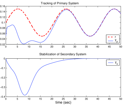
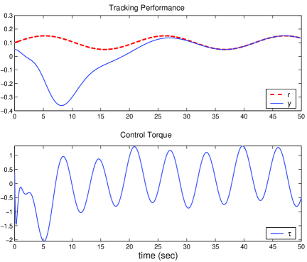
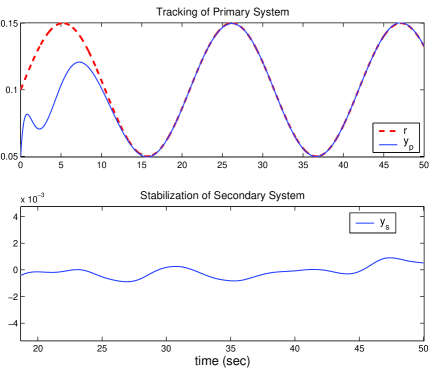
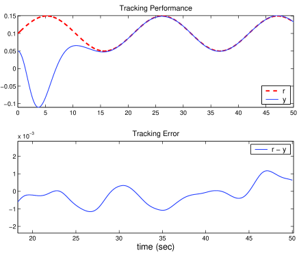
First, let us see the control performance of the primary system (21) and the secondary system (22) in Case 1 (sinusoidal disturbance). The evolutions of their outputs are shown in Fig.3. As shown, it can be seen that $y_{p}=y_{pp}+y_{ps}\rightarrow r$ as $t\rightarrow\infty$ and $y_{s}\rightarrow 0$ as $t\rightarrow\infty$. Therefore, by the additive state decomposition, $y=y_{p}+y_{s}\rightarrow r$ as $t\rightarrow\infty$. This is confirmed by the simulation shown in Fig.4. Secondly, let us see the control performance of the primary system (21) and the secondary system (22) in Case 2 (general disturbance). The evolutions of their outputs are shown in Fig.5. As shown, it can be seen that $y_{p}$ tracks $r$ with good performance and $y_{s}$ is ultimately bounded by a small value. Therefore, by the additive state decomposition, $y=y_{p}+y_{s}$ tracks $r$ with a good performance. This is confirmed by the simulation in Fig.6.

Remark 10. By the additive-state-decomposition-based tracking control scheme, it is seen from the simulation that the transfer function method is applied to the tracking controller design, which increases flexibility of the design. By benefiting from it, both a sinusoidal and a general disturbance can be handled in the same framework, where only the subcontroller $u^{d}$ needs to be modified rather than the whole one.

VI Conclusions

In this paper, the output feedback tracking problem for a class of systems with measurable nonlinearities and unknown disturbances was considered. Our main contribution lies in the presentation of a new decomposition scheme, named additive state decomposition, which not only simplifies the controller design but also increases flexibility of the controller design.

The proposed additive-state-decomposition-based tracking control scheme was adopted to solve the output feedback tracking problem. First, the considered system was transformed to an input-output equivalent disturbance-free system. Then, by the additive state decomposition, the transformed system was decomposed into three subsystems in charge of three independent subtasks respectively: an LTI system in charge of a pure tracking subtask, another LTI system in charge of a pure rejection subtask and a nonlinear system in charge of a stabilization subtask. Based on the decomposition, the subcontrollers corresponding to three subsystems were designed separately, which increases the flexibility of design. To demonstrate its effectiveness, the proposed additive-state-decomposition-based tracking control was applied to the output feedback tracking problem for a single-link robot arm with a revolute elastic joint rotating in a vertical plane.

VII Appendix: Proof of Theorem 4

It is easy to follow the proof in Theorems 2-3 that the observer (37) will make

$\displaystyle\hat{x}_{new}$ $\displaystyle\equiv x_{new},\hat{d}_{new}\equiv d_{new},\hat{x}_{p}\equiv x_{p},$
$\displaystyle\hat{x}_{s}$ $\displaystyle\equiv x_{s},\hat{x}_{pp}\equiv x_{pp},\hat{x}_{ps}\equiv x_{ps}.$ (39)

The remainder proof is composed of two parts: i) for (21), the controller $u_{p}$ drives $y_{p}\rightarrow r+\mathcal{B}\left(\delta\right)$ as $t\rightarrow\infty$, and ii) based on the result of i), for (22), the controller $u_{s}$ drives $y_{s}\rightarrow\mathcal{B}\left(\left\|c\right\|\gamma\left(\delta\right)\right)$ as $t\rightarrow\infty.$ Then the controller $u=u_{p}+u_{s}$ drives $y\rightarrow r+\mathcal{B}\left(\delta+\left\|c\right\|\gamma\left(\delta\right)\right)$ as $t\rightarrow\infty$ in system (1) (or (12)).

i) Suppose that Problems 1-2 are solved. By (28) and (39), the controller $u_{pp}$ is designed as follows:

$\displaystyle\dot{z}^{r}$ $\displaystyle=\alpha^{r}\left(z^{r},\hat{x}_{pp},r\right),z^{r}\left(0\right)=0$
$\displaystyle u_{pp}$ $\displaystyle=u^{r}\left(z^{r},\hat{x}_{pp},r\right)$

which can drive $y_{pp}\rightarrow r$ as $t\rightarrow\infty$ in (25). By (30) and (39), the controller $u_{ps}$ is designed as follows:

$\displaystyle\dot{z}^{d}$ $\displaystyle=\alpha^{d}\left(z^{d},\hat{x}_{ps},\hat{d}_{new}\right),z^{d}\left(0\right)=0$
$\displaystyle u_{ps}$ $\displaystyle=u^{d}\left(z^{d},\hat{x}_{ps},\hat{d}_{new}\right)$

which will drive $y_{ps}\rightarrow\mathcal{B}\left(\delta\right)$ as $t\rightarrow\infty$ in (26). Combining the two controllers $u_{pp}$ and $u_{ps}$ above results in the controller for the primary system (21):

$\displaystyle\dot{z}^{r}$ $\displaystyle=\alpha^{r}\left(z^{r},\hat{x}_{pp},r\right),z^{r}\left(0\right)=0$
$\displaystyle\dot{z}^{d}$ $\displaystyle=\alpha^{d}\left(z^{d},\hat{x}_{ps},\hat{d}_{new}\right),z^{d}\left(0\right)=0$
$\displaystyle u_{p}$ $\displaystyle=u^{r}\left(z^{r},\hat{x}_{pp},r\right)+u^{d}\left(z^{d},\hat{x}_{ps},\hat{d}_{new}\right).$ (40)

Therefore, by (27), the controller (40) can drive $y_{p}\rightarrow r+\mathcal{B}\left(\delta\right)$ as $t\rightarrow\infty$.

ii) Let us look at the secondary system (22). Suppose that Problems 3 is solved. By (39), the controller $u_{s}=u^{s}\left(\hat{x}_{s},r,\cdots,r^{\left(N\right)}\right)$ can drive the output $y_{s}$ such that

$\displaystyle\left\|y_{s}\left(t\right)\right\|$ $\displaystyle\leq\left\|c\right\|\left\|x_{s}\left(t\right)\right\|$
$\displaystyle\leq\left\|c\right\|\beta\left(\left\|x_{s}\left(t_{0}\right)\right\|,t-t_{0}\right)+\left\|c\right\|\gamma\left(\underset{t_{0}\leq s\leq t}{\sup}\left\|e_{p}\left(s\right)\right\|\right),t\geq 0.$

Based on the result of i), we get $e_{p}\rightarrow\mathcal{B}\left(\delta\right)$ as $t\rightarrow\infty.$ This implies that $\left\|e_{p}\left(t\right)\right\|\leq\delta+\varepsilon$ when $t\geq t_{0}+T_{1}.$ Then

$\displaystyle\left\|y_{s}\left(t\right)\right\|$ $\displaystyle\leq\left\|c\right\|\beta\left(\left\|x_{s}\left(t_{0}+T_{1}\right)\right\|,t-t_{0}-T_{1}\right)+\left\|c\right\|\gamma\left(\underset{t_{0}+T_{1}\leq s\leq t}{\sup}\left\|e_{p}\left(s\right)\right\|\right),t\geq t_{0}+T_{1},$
$\displaystyle\leq\left\|c\right\|\beta\left(\left\|x_{s}\left(t_{0}+T_{1}\right)\right\|,t-t_{0}-T_{1}\right)+\left\|c\right\|\gamma\left(\delta+\varepsilon\right),t\geq t_{0}+T_{1}.$

Since $\left\|c\right\|\beta\left(\left\|x_{s}\left(t_{0}+T_{1}\right)\right\|,t-t_{0}-T_{1}\right)\rightarrow 0$ as $t\rightarrow\infty$ and $\varepsilon$ can be chosen arbitrarily small, we can conclude $y_{s}\rightarrow\mathcal{B}\left(\left\|c\right\|\gamma\left(\delta\right)\right)$ as $t\rightarrow\infty.$ Since $y=c^{T}x_{p}+c^{T}x_{s},$ we can conclude that, driven by the controller (38), the output of the system (1) (or (12)) satisfies that $y\rightarrow r+\mathcal{B}\left(\delta+\left\|c\right\|\gamma\left(\delta\right)\right)$ as $t\rightarrow\infty$. In particular, if $\delta=0,$ then the output in system ((12)) satisfies that $y\rightarrow r$ as $t\rightarrow\infty.$ $\square$

References

  • [1] Ding Z. Global stabilization and disturbance suppression of a class of nonlinear systems with uncertain internal model. Automatica 2003; 39 (3): 471–479.
  • [2] Marino R, Tomei P. Adaptive tracking and disturbance rejection for uncertain nonlinear systems. IEEE Transactions on Automatic Control 2005; 50 (1): 90–95.
  • [3] Marino R, Santosuosso GL. Global compensation of unknown sinusoidal disturbances for a class of nonlinear nonminimum phase systems. IEEE Transactions on Automatic Control 2005; 50 (11): 1816–1822.
  • [4] Ding Z. Adaptive estimation and rejection of unknown sinusoidal disturbances in a class of non-minimum-phase nonlinear systems. IEE Proceedings Control Theory & Applications 2006; 153 (4): 379–386.
  • [5] Lan W, Chen BM, Ding Z. Adaptive estimation and rejection of unknown sinusoidal disturbances through measurement feedback for a class of non-minimum phase non-linear MIMO systems. International Journal of Adaptive Control and Signal Processing 2006; 20 (2): 77–97.
  • [6] Marino R, Santosuosso GL, Tomei P. Two global regulators for systems with measurable nonlinearities and unknown sinusoidal disturbances. Analysis and Design of Nonlinear Control Systems: in Honor of Alberto Isidori, Astolfi, A., & Marconi, R. (eds.). Berlin: Springer, 2008.
  • [7] Bobtsov AA, Kremlev AS, Pyrkin AA. Compensation of harmonic disturbances in nonlinear plants with parametric and functional uncertainty. Automation and Remote Control 2011; 72 (1): 111–118.
  • [8] Chen J. Sensitivity integral relations and design trade-offs in linear multivariable feedback systems. IEEE Transactions On Automatic Control 1995; 40 (10): 1700–1716.
  • [9] Zhou K, Doyle JC, Glover KH. Robust and Optimal Control. Upper Saddle River, NJ: Prentice-Hall, 1996.
  • [10] Francis BA, Wonham WM. The internal model principle of control theory. Automatica 1976; 12 (5): 457–465.
  • [11] Morari M, Zafiriou E. Robust Process Control (1st ed.). Upper Saddle River, NJ: Prentice-Hall, 1989.
  • [12] Quan Q, Cai K-Y. Additive decomposition and its applications to internal-model-based tracking. Joint 48th IEEE Conference on Decision and Control and 28th Chinese Control Conference, Shanghai, China, 817–822, 2009.
  • [13] Fradkov AL, Miroshnik IV, Nikiforov VO. Nonlinear and Adaptive Control of Complex Systems. Boston: Kluwer Academic, 1999.
  • [14] Zhu W-H. Virtual Decomposition Control: Toward Hyper Degrees of Freedom Robots. New York: Springer, 2010.
  • [15] Marino R, Tomei P. Global adaptive output-feedback control of nonlinear systems, part I: Linear parameterization. IEEE Transactions on Automatic Control 1993; 38 (1): 17–32.
  • [16] Marino R, Tomei P. Nonlinear Control Design: Geometric, Adaptive and Robust. London: Prentice Hall, 1995.
  • [17] Devasia S, Chen D, Paden B. Nonlinear inversion-based output tracking. IEEE Transactions on Automatic Control 1996; 41 (7): 930–942.
  • [18] Hunt LR, Meye G. Stable inversion for nonlinear systems. Automatica 1997; 33 (8): 1549–1554.
  • [19] Khalil HK. Nonlinear Systems. Upper Saddle River, NJ: Prentice-Hall, 2002.
  • [20] Sontag ED. Input to state stability: Basic concepts and results. In Nonlinear and Optimal Control Theory, P. Nistri and G. Stefani, Eds. Berlin, Germany: Springer-Verlag, 2007, pp. 166–220.
  • [21] Sussmann HJ, Kokotovic PV. The peaking phenomenon and the global stabilization of nonlinear systems. IEEE Transactions on Automatic Control 1991; 36 (4): 424–440.
Refer to caption
Figure 2: Disturbance in Case 2
Refer to caption
Figure 3: Outputs of primary system and secondary system in Case 1
Refer to caption
Figure 4: Output (link displacement) of the single-link robot arm and control toque in Case 1
Refer to caption
Figure 5: Outputs of primary system and secondary system in Case 2
Refer to caption
Figure 6: Output (link displacement) of the single-link robot arm in Case 2