Itinerant and local-moment magnetism in strongly correlated electron systems

Abstract

Detailed analysis of the magnetic properties of the Hubbard model within dynamical mean-field theory (DMFT) is presented. Using a RPA-like decoupling of two-particle propagators we derive an universal form for susceptibilities, which captures essential aspects of localized and itinerant pictures. This expression is shown to be quantitatively valid whenever long-range coherence of particle-hole excitations can be neglected, as is the case in large parts of the phase diagram where antiferromagnetism is dominant. The applicability of an interpretation in terms of the two archetypical pictures of magnetism is investigated for the Hubbard model on a body-centered cubic lattice with additional next-nearest neighbor hopping $t^{\prime}$. For large values of the Coulomb interaction, local-moment magnetism is found to be dominant, while for weakly interacting band electrons itinerant quasiparticle magnetism prevails. In the intermediate regime and for finite $t^{\prime}$ an re-entrant behavior is discovered, where antiferromagnetism only exists in a finite temperature interval.

I Introduction

The magnetic properties of solids are typically described in terms of two archetypical and opposing viewpoints. On the one hand, the picture of weakly interacting itinerant electron magnetism is usually implemented for metallic systems. On the other hand, for small overlap between sites or for strong local interactions the valence electrons can form localized moments and behave effectively like spin degrees of freedom of a Heisenberg model (for introductory texts, see, for example, Refs. Fazekas, 1999 and Yosida, 1996).

In strongly correlated electron systems, such as cuprate high-temperature superconductorsPlakida (2010) or heavy fermion systems,Grewe and Steglich (1991); *colemanHeavyFermionMag07 such a clear distinction is often obscured since aspects of both pictures appear. Due to the strong Coulomb interaction the electrons are rather localized furnishing large magnetic moments. However, at low temperatures usually a bandstructure of heavy but itinerant quasiparticles around the Fermi level forms, giving rise to the screening of local moments. Central to the magnetic properties in these systems is the competition between quasiparticle-band formation, possibly spin-polarized, and ordering tendencies of large local moments.

This competition yields especially interesting and novel physics in the case of frustrated systems.Lacroix et al. (2011) In the recently studied frustrated heavy fermion systems, such as LiV₂O₄, frustrated local moments dominate at elevated temperatures, while at low temperatures strongly correlated quasiparticles emerge (see, for example, Ref. Hopkinson and Coleman, 2002; *joenssonLiV2O407; *aritaLiV2O407). Similarly, a competition between frustrated magnetic moments and a low temperature Fermi liquid has been proposed as an explanation for the re-entrant Mott-transition found in the highly frustrated organic compound $\kappa$-(ET)₂Cu[N(CN)₂]Cl.Kagawa et al. (2004); *ohashiTriangularHM08; *ohashiTriangularHM08-2 In the context of the cuprate high-temperature superconductors there is a longstanding question whether the magnetic properties are best described in the local or itinerant picture, see, for example, Ref. Vojta, 2009. Due to the proximity of these systems to the Mott-insulating phase, the localized picture is often proposed, whereas recent studies also revealed the presence of itinerant spin-fluctuations throughout the whole Brillouin zone.He et al. (2011); *taconParamagnonHTC11

In the Hubbard model, all these aspects can be captured. Weakly interacting band electrons can be studied for small values of the Coulomb repulsion. With increasing interaction strength the system undergoes a Mott metal-insulator transition above which it is best characterized by an effective Heisenberg spin model. The interesting region is close to the Mott transition where large magnetic moments and itinerant quasiparticles compete. Frustration effects can be studied by considering, for example, the influence of a next-nearest neighbor hopping in an otherwise bipartite lattice.

The magnetic properties of the Hubbard model are very well studied. Even though the model was introduced in order to describe ferromagnetism (FM) this phase is restricted to very large interaction strength and depends on details of the bandstructure.Vollhardt et al. (1999); Fazekas (1999) Antiferromagnetism (AFM), however, represents a generic phase of the model and is found in large regions of phase space.Fazekas (1999)

A very useful method to study the Hubbard model in the strongly correlated regime near the Mott transition is provided by the dynamical mean field theoryPruschke et al. (1995); *georges:dmft96; *georgesDMFTreview04 (DMFT). With this method one can access the single-particle Green function as well as two-particle quantities like susceptibilities.

We will consider the Bethe-Salpeter equations and derive coupled equations for dynamic lattice susceptibilities which prove equivalent to the usual expression known from the DMFT,Jarrell (1992); Zlatic and Horvatic (1990); *jarrell:symmetricPAM95 but lend themselves more directly to our specific investigation of magnetism. The ultimate goal of this approach is to analytical continue these equations directly to the real axis and obtain integral equations for functions of real frequency arguments.

In this work, however, we employ an additional decoupling scheme for the internal Matsubara summations which allows us to derive an universal approximation for the susceptibility, which unifies localized and itinerant aspects of magnetism. We discuss the range of validity of this formula and demonstrate its accurateness by reproducing the DMFT Néel temperature for the Hubbard model on a simple cubic (SC) lattice in three dimensions, $D=3$. The appeal of this approach lies in its simplicity compared to the usual Matsubara approach to two-particle properties.Toschi et al. (2007); Kuneš (2011) Only functions of real frequencies enter and the inversions of Matsubara-space matrices is avoided.

The competition between local-moment and itinerant quasiparticle magnetism is studied for a three-dimensional body-centered cubic (BCC) lattice with an additional next-nearest neighbor hopping $t^{\prime}$. In situations where quasiparticle magnetism is dominant, the tendency toward magnetic order should be strongly suppressed by a finite next-nearest neighbor hopping, since the perfect nesting property of the Fermi surface is removed. On the other hand, local-moment magnetism is less sensitive since the geometric frustration induced by the next-nearest neighbor hopping reduces the effective exchange coupling only quadratically in $t^{\prime}$. This behavior is indeed found for weak and strong Coulomb repulsions, respectively. In the crossover region for intermediate interactions, an interesting re-entrant behavior is found where the effective picture to be used depends on the temperature of the system. Crucial to the occurrence of this behavior is the presence of the frustrating next-nearest neighbor hopping $t^{\prime}$. The findings of this work are in accord with the common believe that frustration is capable of producing novel and interesting phenomena.

The paper is organized as follows. After a brief introduction of the model, Sect. II sketches the derivation of the Bethe-Salpeter equations for lattice susceptibilities. We present two different interpretations of the resulting simple formula for the magnetic susceptibility, one in terms of local moments and the other utilizing itinerant quasiparticles. In the first part of Sect. III we investigate the validity of our approach and compare the Néel temperature for the SC lattice to known results from the literature. The second part of this section then focuses on the BCC lattice where the magnetic properties are investigated in detail. We also include two appendices, where more details on the technicalities are presented. The focus is laid on the similarities and differences of the the single-particle and two-particle set-up.

II Model and Method

In metals the long-ranged Coulomb interaction is usually screened and only short-range components have to be considered. In order to study the effects of electronic correlations we consider the Hubbard model, where only the on-site Coulomb repulsion is retained. For the sake of simplicity, we assume ionic $s$-shells without orbital degeneracy and with remaining spin-degeneracy only, although the formal developments described below can easily be generalized.

The Hamiltonian is given by

$$\hat{H} =\sum_{ij,\sigma}t_{ij}\hat{c}^{\dagger}_{i\sigma}\hat{c}^{\phantom{\dagger}}_{j\sigma}+\sum_{i\,\sigma}\epsilon\>\hat{c}^{\dagger}_{i\sigma}\hat{c}^{\phantom{\dagger}}_{i\sigma}+U\,\sum_{i}\hat{n}_{i\uparrow}\hat{n}_{i\downarrow},$$ (1)

where the operator $\hat{c}^{\phantom{\dagger}}_{i\sigma}$ ($\hat{c}^{\dagger}_{i\sigma}$) annihilates (creates) an electron in a localized Wannier orbital at lattice site $i$ with spin $\sigma$, $\hat{n}_{i\sigma}=\hat{c}^{\dagger}_{i\sigma}\hat{c}^{\phantom{\dagger}}_{i\sigma}$ is the number operator and $\epsilon$ is the ionic level position where the chemical potential is already taken into account. The electrons can transfer between sites $i$ and $j$ with an amplitude $t_{ij}$, which accounts for the itinerancy and band formation of the electrons. The last term in Eq. (1) implements the local Coulomb repulsion with the interaction matrix element $U$.

The structure of the lattice is encoded into the one-particle hopping amplitude $t_{ij}$, the Fourier transform of which gives the single-particle dispersion relation

$$t_{\underline{k}} =\frac{1}{N}\sum_{jl}e^{i({\underline{R}}_{j}-{\underline{R}}_{l}){\underline{k}}}\>t_{jl}.$$ (2)

The noninteracting density of states (DOS) is entirely determined by the dispersion relation

$$\rho_{0}(\omega) =\frac{1}{N}\sum_{{\underline{k}}}\delta(\omega-t_{\underline{k}}).$$ (3)

Despite its simplicity, the exact solution of the Hubbard Hamiltonian of Eq. (1) is only possible in one spatial dimensionLieb and Wu (1968); *lieb1DHubbard03 (for a recent book, see, e.g., Ref. Essler et al., 2005) and in infinite spatial dimensions, $D\to\infty$ (with an appropriate rescaling the hopping parameters),Metzner and Vollhardt (1989); *muellerHartmannDInfty89 by means of the DMFT. In this work we will utilize DMFT in order to extract an approximate solution for three dimensional systems.

In finite dimensions the major approximation of DMFT is to treat all spatially nonlocal correlations in a mean-field manner. For the single-particle properties, this implies the assumption of a momentum independent interaction self-energy, $\Sigma^{U}({\underline{k}},z)\overset{\mathrm{DMFT}}{\to}\Sigma^{U}(z)$. Then, the structure and dimensionality of the lattice enters the lattice Green function only via the dispersion relation,

$$G({\underline{k}},z)=\frac{1}{z-\Sigma^{U}(z)-t_{\underline{k}}}.$$ (4)

However, the dependence on the (complex) energy variable $z$ is not neglected and thus dynamic local correlations are fully retained within DMFT. The self-energy and the local Green function,

$$G(z) =\frac{1}{N}\sum_{{\underline{k}}}\frac{1}{z-\Sigma^{U}(z)-t_{{\underline{k}}}}$$ (5)

$$=\frac{1}{z-\Sigma^{U}(z)-\Gamma(z)}$$ (6)

can be obtained from an effective single-impurity Anderson model (SIAM) embedded in a self-consistent medium characterized by the hybridization function $\Gamma(z)$. Once the effective SIAM is solved for a given $\Gamma(z)$, a new guess for the self-energy is obtained by inverting Eq. (6), which in turn is used to get $G(z)$ via Eq. (5). Only in this last step the lattice structure enters. The self-consistency cycle is closed by reorganizing Eq. (6) and extracting a new guess for $\Gamma(z)$.

The nontrivial part in this cycle is the solution of the effective SIAM. But due to its long history, a multitude of different methods for treating this model exist, for example, exact diagonalization,Caffarel and Krauth (1994); *Si1994 several variations of quantum Monte-Carlo schemes,Hirsch and Fye (1986); *gullCTQMC11 and the numerical renormalization groupWilson (1975); *bullaNRGReview08 (NRG). In this work, we employ the enhanced non-crossing approximationPruschke and Grewe (1989); *schmittSus09; *greweCA108; Holm and Schönhammer (1989); *keiterENCA90 (ENCA), which has no adjustable parameters and works directly on the real frequency axis.

The tendency toward magnetism is investigated via the magnetic susceptibility of the paramagnetic phase, which diverges at a second order phase transition. The susceptibility is given by the nonlocal time-dependent order-parameter correlation function

$$\chi^{\mathrm{mag}}_{ij}(\tau) =\langle\mathcal{T}\big{[}\hat{M}_{i}^{z}(\tau)\,\hat{M}_{j}^{z}(0)\big{]}\rangle,$$ (7)

with the total magnetization operator at lattice site $i$

$$\hat{M}^{z}_{i} =\sum_{a}\gamma_{a}\>\hat{n}^{\phantom{\dagger}}_{ia}.$$ (8)

In general, the index $a$ denotes orbital and spin quantum numbers. With the assumption of $s$-shells one has especially $a=\sigma$ and $\gamma_{\sigma}=-\frac{g\mu_{B}}{2}\sigma$, where $g$ is the electron Landé factor and $\mu_{B}$ the Bohr magneton.

Equation (7) is already specified to isotropic situations where the susceptibility tensor is diagonal and all diagonal elements are equal, i.e. $\chi_{ij}^{\mathrm{mag};\alpha\beta}=\chi_{ij}^{\mathrm{mag}}\>\delta_{\alpha\beta}$ ($\alpha,\beta=\{x,y,z\}$). For a paramagnetic situation, the transverse susceptibility is just given by twice this value, $\chi_{ij}^{\mathrm{mag};\perp}=2\chi_{ij}^{\mathrm{mag}}$.

The wave-vector and frequency dependent susceptibility is obtained by the Fourier transform of Eq. (7),

$$\chi_{\mathrm{mag}}({\underline{q}},i\nu_{n})=\frac{1}{(N)^{2}}\sum_{ij}\int_{0}^{\beta}\!d\tau\>e^{i\nu_{n}\tau}\>e^{i{\underline{q}}({\underline{R}}_{i}-{\underline{R}}_{j})}\chi_{ij}(\tau)$$

$$=\sum_{ab}\gamma_{a}\gamma_{b}\Big{\{}\langle\hat{n}_{a}\rangle\langle\hat{n}_{b}\rangle\>\delta_{i\nu_{n},0}+\Big{[}\uuline{\chi}{}({\underline{q}},i\nu_{n})\Big{]}_{abba}\Big{\}}.$$ (9)

where $\nu_{n}=\frac{2\pi}{\beta}n$ ($n\in\mathbb{Z}$) are bosonic Matsubara frequencies and $\beta=\frac{1}{k_{\mathrm{B}}T}$ the inverse temperature $T$. We already separated the static ($i\nu_{n}=0$) unconnected part proportional to a product of local occupation numbers $\langle\hat{n}_{a}\rangle$ in the first term.

We introduced a matrix notation in orbital space for the Fourier transform of the connected two-particle Green function, $\uuline{\chi}{}({\underline{q}},i\nu_{n})=\{\chi_{a,b;c,d}({\underline{q}},i\nu_{n})\}$ (see Appendix B). This is the central quantity of interest, as other particle-hole susceptibilities can equally well be calculated from it. The charge susceptibility, for example, is obtained by using different matrix elements $\gamma_{\sigma}=-|e|$ in Eq. (8), which amounts to a different sum over the matrix elements of the susceptibility matrix in Eq. (9). Therefore, we will focus in the following on the susceptibility matrix $\uuline{\chi}{}({\underline{q}},i\nu_{n})$, without the specific pre-factors $\gamma_{a}$ unless needed, i.e. for their signs.

In analogy to the self-energy, the particle-hole irreducible two-particle interaction vertex is assumed to be momentum independent within DMFT,Jarrell (1992); Zlatic and Horvatic (1990); *jarrell:symmetricPAM95

$$\uuline{\Pi}{}(i\omega_{1},{\underline{k}}_{1},i\omega_{2},{\underline{k}}_{2};i\omega_{2}^{\prime},{\underline{k}}_{2}^{\prime},i\omega_{1}^{\prime},{\underline{k}}_{1}^{\prime})$$ (10)

$$\overset{\text{DMFT}}{\to}\uuline{\Pi}{}(i\omega_{1},i\omega_{2};i\omega_{2}^{\prime},i\omega_{1}^{\prime}).$$

As a consequence, sums over crystal momentum only involve the one-particle propagators leading to simple local expressions for closed loops or a geometric series for chains through the lattice. At interaction points crystal momentum is only conserved on average. A similar procedure fails for internal Matsubara sums since all frequency dependencies are retained within DMFT. Therefore, the Bethe-Salpeter equations, as detailed in the appendix, have the structure of coupled integral equations in Matsubara frequency space.

The dynamic susceptibility is obtained by summing the appropriate two-particle Green function over two internal frequencies,

$$\uuline{\chi}{}({\underline{q}},i\nu_{n})=\frac{1}{\beta}\sum_{i\omega_{1},i\omega_{2}}\uuline{\chi}{}({\underline{q}},i\nu_{n}|i\omega_{1},i\omega_{2})\>e^{(i\omega_{1}\!+i\omega_{2})\delta}.$$ (11)

The exponential incorporates infinitesimal convergence factors $\delta$ which ensure the correct time ordering of the number-operators in the two-particle Green function.

Frequently, in particular when using QMC as impurity solver, the two-particle lattice susceptibility is obtained by interpreting Green functions as matrices in Matsubara frequency space, $\uuline{\chi}{}({\underline{q}},i\nu_{n}|i\omega_{1},i\omega_{2})=\uuline{\hat{\chi}}{}_{{\underline{q}},i\nu_{n}}|_{\omega_{1},\omega_{2}}$ (indicated by a hat and the different placement of the external variable in our notation). The Bethe-Salpeter equation then has the structure of a matrix equation, where the internal frequency sums are represented by matrix multiplications,

$$\uuline{\hat{\chi}}{}_{{\underline{q}},i\nu_{n}}=-\uuline{\hat{P}}{}_{{\underline{q}},i\nu_{n}}-\uuline{\hat{P}}{}_{{\underline{q}},i\nu_{n}}\uuline{\hat{\Pi}}{}_{i\nu_{n}}\uuline{\hat{\chi}}{}_{{\underline{q}},i\nu_{n}}.$$ (12)

The particle-hole propagator $\uuline{\hat{P}}{}_{{\underline{q}},\nu_{n}}$ is determined by the single-particle Green function (cf. Eq. (72)), and explicit two-particle interactions are incorporated via the irreducible vertex $\uuline{\hat{\Pi}}{}_{\nu_{n}}$, which is a priori unknown and hard to calculate directly for strongly correlated systems.

For a description via effective impurities underlying the DMFT-method, an analogous equation can be formulated,

$$\uuline{\hat{\chi}}{}^{\mathrm{loc}}_{i\nu_{n}}=-\uuline{\hat{P}}{}^{\mathrm{loc}}_{i\nu_{n}}-\uuline{\hat{P}}{}^{\mathrm{loc}}_{i\nu_{n}}\,\uuline{\hat{\Pi}}{}_{i\nu_{n}}\,\uuline{\hat{\chi}}{}^{\mathrm{loc}}_{i\nu_{n}}.$$ (13)

$\uuline{\hat{\chi}}{}^{\mathrm{loc}}_{i\nu_{n}}$ is the dynamic local susceptibility of the effective impurity model and can be calculated in principle. The local particle-hole propagator is given by the momentum sum of its lattice counter part,

$$\uuline{\hat{P}}{}^{\mathrm{loc}}_{i\nu_{n}}=\frac{1}{N}\sum_{q}\uuline{\hat{P}}{}_{{\underline{q}},i\nu_{n}},$$ (14)

and can be calculated with knowledge of the local Green function (see Eq. (71)).

The same irreducible local vertex $\uuline{\hat{\Pi}}{}_{i\nu_{n}}$ is assumed for the impurity and the lattice model. This makes it possible to eliminate it from Eqs. (13) and (12) and the usual DMFT result for the lattice susceptibility is obtained

$$\uuline{\hat{\chi}}{}_{{\underline{q}},i\nu_{n}}=\left[-\uuline{\hat{P}}{}_{{\underline{q}},i\nu_{n}}^{-1}+{\uuline{\hat{\chi}}{}^{\mathrm{loc}}_{i\nu_{n}}}^{-1}+{\uuline{\hat{P}}{}^{\mathrm{loc}}_{i\nu_{n}}}^{-1}\right]^{-1}.$$ (15)

The inversions indicate matrix inversions in the space of Matsubara frequencies and orbital/spin space. It is important to realize that all quantities entering Eq. (15) can be calculated directly from the effective impurity model and the lattice Green function. One thus has an explicit equation for the lattice susceptibility.

However, the shortcoming of the approach sketched above is twofold. First, the set of Matsubara frequencies $i\omega_{n}$ is infinite as $n\in\mathbb{Z}$. The Matsubara matrices are therefore infinite dimensional, which is of course not sustainable in practical calculations and truncations have to be introduced. Second, the calculated susceptibilities are functions of complex Matsubara frequencies which have to be numerically continued to the real axis which is mathematically an ill-defined problem. There exist sophisticated techniques, such as maximum entropy methods,Jarrell and Gubernatis (1996) but uncertainties and uncontrolled errors remain.

Another approach utilizes the dynamic density-matrix renormalization group technique and a subsequent deconvolution.Raas and Uhrig (2005); *raasGenSus09 Apart from being very resource consuming, the deconvolution to obtain data on the real frequency axis might also introduce artefacts.

In order to avoid these difficulties we take a different route here. We introduce an additional approximation and decouple the Matsubara sums in the Bethe-Salpeter equations in a manner similar to the random-phase approximation (RPA). For technical details see appendix B. The major advantage is that the analytic continuation of all frequency variables to the real axis, like $i\nu_{n}\to\nu+i\delta$, can be done analytically. As derived in the appendix, the result isSchmitt and Grewe (2005); Schmitt (2009)

$$\uuline{\chi}{}({\underline{q}},\nu)=$$ (16)

$$\Big{[}-\uuline{P}{}({\underline{q}},\nu)^{-1}+{\uuline{\chi}{}^{\mathrm{loc}}(\nu)}^{-1}+{\uuline{P}{}^{\mathrm{loc}}(\nu)}^{-1}\Big{]}^{-1}.$$

The structure of this equation is of course the same as Eq. (15), but the important difference is that no Matsubara matrices occur (there are no hats are over the quantities) and the external frequency $\nu$ is a real variable. The indicated matrix structure and inversions only refer to the orbital/spin space.

In the following we will focus on the magnetic susceptibility and on simple $s$-shells. In that case, all quantities are matrices in spin-space only. The particle-hole propagators of the paramagnetic regime are spin-symmetric, $P_{\uparrow}=P_{\downarrow}\equiv P$, and only two independent components exist for the susceptibilities, $\chi_{\uparrow,\uparrow;\uparrow,\uparrow}=\chi_{\downarrow,\downarrow;\downarrow,\downarrow}$ and $\chi_{\uparrow,\downarrow;\downarrow,\uparrow}=\chi_{\downarrow,\uparrow;\uparrow,\downarrow}$. The magnetic susceptibility is a linear combination of these two components, $\chi_{\mathrm{mag}}({\underline{q}},\nu)=\chi_{\uparrow,\uparrow;\uparrow,\uparrow}({\underline{q}},\nu)-\chi_{\uparrow,\downarrow;\downarrow,\uparrow}({\underline{q}},\nu)$, and can be expressed as (neglecting the prefactor $(\frac{g\mu_{B}}{2})^{2}$),

$$\chi_{\mathrm{mag}}({\underline{q}},\nu) =\Big{[}-\frac{1}{P({\underline{q}},\nu)}+\frac{1}{P^{\mathrm{loc}}(\nu)}+\frac{1}{\chi^{\mathrm{loc}}_{\mathrm{mag}}(\nu)}\Big{]}^{-1}.$$ (17)

All quantities entering this form are scalar functions of a real variable. $\chi^{\mathrm{loc}}_{\mathrm{mag}}(\nu)$ is the dynamic local magnetic susceptibility of the impurity model, $P^{\mathrm{loc}}(\nu)$ and $P({\underline{q}},\nu)$ are the local and lattice dependent particle-hole propagators, which only depend on the fully interacting single-particle Green function (see Eqs. (71) and (72)).

This specific form (17) for the susceptibility lends itself directly to interpretations in terms of the two archetypical physical pictures underlying magnetism:

• The picture of local-moment magnetism is suggested if Eq. (17) is re-written as

  $$\chi_{\mathrm{mag}}({\underline{q}},\nu) =\frac{\chi^{\mathrm{loc}}_{\text{mag}}(\nu)}{1-J({\underline{q}},\nu)\,\chi^{\mathrm{loc}}_{\text{mag}}(\nu)},$$ (17a)

  where local spins characterized by $\chi^{\mathrm{loc}}_{\text{mag}}$ interact via a nonlocal and dynamic exchange coupling

  $$J({\underline{q}},\nu) =\frac{1}{P({\underline{q}},\nu)}-\frac{1}{P^{\mathrm{loc}}(\nu)}.$$ (18)

  This view is substantiated by approaching the atomic limit. Then, the hopping matrix elements vanish, $t_{\underline{k}}=0$, and the lattice and the local particle-hole propagators become identical, $P({\underline{q}},\nu)|^{t=0}=P^{\mathrm{loc}}(\nu)$. The susceptibility correctly reduces to the fully interacting susceptibility of isolated ions,

  $$\chi_{\mathrm{mag}}({\underline{q}},\nu)|^{t=0} =\chi_{\mathrm{mag}}^{\mathrm{loc}}(\nu).$$ (19)

  For half-filling and $U>0$ it is just given by that of a free spin

  $$\chi_{\mathrm{mag}}({\underline{q}},\nu)|^{t=0} =\frac{1}{T}\,\delta(\nu).$$ (20)

  This result is easily extended to incorporate the leading order correction due to the coupling to neighboring ions. Expanding up to second order in the hopping around the atomic limit yields the exchange coupling $J({\underline{q}},\nu)=\frac{1}{U}\frac{1}{N}\sum_{\underline{k}}t_{\underline{k}}\,t_{{\underline{k}}+{\underline{q}}}+\mathcal{O}(t^{3})$. The susceptibility then correctly reproduces the the mean-field approximation to the Heisenberg model,

  $$\chi_{\mathrm{mag}}({\underline{q}},\nu)=\frac{1}{T-T_{C}({\underline{q}})}\,\delta(\nu)+\mathcal{O}(t^{3}).$$ (21)

  In case of a simple-cubic lattice with nearest hopping, the $T_{C}({\underline{q}})$ is given by $T_{C}({\underline{q}})=-\frac{2t^{2}}{U}\sum_{i=1}^{D}\cos(q_{i})$. This reproduces the AFM ${\underline{Q}}=\pi(1,1,\dots)^{T}$ mean-field transition at the well-known critical temperature $T_{C}({\underline{Q}})=\frac{2Dt^{2}}{U}$.

• The interpretation in terms of the itinerant picture of magnetism is obtained by re-writing Eq. (17) as

  $$\chi_{\mathrm{mag}}({\underline{q}},\nu) =\frac{-P({\underline{q}},\nu)}{1+\Gamma_{\mathrm{mag}}(\nu)P({\underline{q}},\nu)}.$$ (17b)

  Here, propagating electrons characterized by their particle-hole susceptibility $-P({\underline{q}},\nu)$ interact locally with the vertex

  $$\Gamma_{\text{mag}}(\nu) =-\frac{1}{\chi_{\mathrm{mag}}^{\mathrm{loc}}(\nu)}-\frac{1}{P^{\mathrm{loc}}(\nu)}.$$ (22)

  This view is substantiated by the noninteracting limit, where the Coulomb interaction matrix element vanishes, $U=0$. Then, Wick’s theorem is applicable and the local susceptibility reduces to the negative local particle-hole propagator $\chi_{\mathrm{mag}}^{\mathrm{loc}}(\nu)|^{U=0}=-P^{\mathrm{loc}}(\nu)$. The susceptibility is then indeed that of noninteracting particles on a lattice given by the Lindhard-function

  $$\chi({\underline{q}},\nu)|^{U=0} =-P({\underline{q}},\nu)|^{U=0}$$ (23)

  $$=-\frac{1}{N}\sum_{\underline{k}}\frac{f(t_{{\underline{k}}+{\underline{q}}})-f(t_{\underline{k}})}{\nu+i0^{+}+t_{{\underline{k}}+{\underline{q}}}-t_{{\underline{k}}}}.$$

  Improving this by employing a perturbation theory in $U$ we arrive at the usual RPA expression. In the lowest order the local vertex is nothing but the bare Coulomb interaction, $\Gamma_{\mathrm{mag}}(\nu)=U$, and then

  $$\chi({\underline{q}},\nu) =\frac{-P({\underline{q}},\nu)|^{U=0}}{1+U\,P({\underline{q}},\nu)|^{U=0}}+\mathcal{O}(U^{2}).$$ (24)

The two opposing cases of a weakly interacting electron gas and the atomic limit are exactly incorporated in the approximate form for the susceptibility, Eq. (17). This substantiates the hope to be able to correctly describe the regime of intermediate coupling strength and especially the transition from itinerant to localized forms of magnetism.

At this point a comment on the advantages and shortcomings of the final expression, Eq. (17), is in place. The major advantage of this formula lies in its simplicity in combination with the correct incorporation of the weak and strong coupling limit. And as it will be shown in the following, the qualitative and quantitative description of correlation effects even for intermediate coupling is very good.

In the usual weak-coupling RPA Doniach and Sondheimer (1974); *schaeferDysonRPAHM99 or extensions thereof, such as the fluctuation exchange approximationBickers et al. (1989); *bickers:ConservingFLEX91 and the two-particle self-consistent approachVilk et al. (1994), the particle-hole propagator is either calculated with bare propagators, i.e. without interactions, or interaction processes are included only at a very crude level. This also applies to auxiliary boson approachesKhaliullin and Horsch (1996); *saikawa:DynamicSusHM98 and equation of motion decoupling schemes.Eremin et al. (2001); *uldryTwoParticleMagSusHM05 In contrast, the particle-hole propagator employed here is calculated with the fully interacting single-particle Green function obtained from DMFT, which incorporates life-time and many-body effects and can already lead to considerable modifications. Furthermore, in the above mentioned approximation schemes the two-particle interaction vertices are given by weighted linear combinations of bare interaction matrix elements, i.e.  by numbers, and the frequency dependence of two-particle vertices is usually ignored. In the present treatment nontrivial dynamic interaction vertices $\Gamma(\nu)$ or $J({\underline{q}},\nu)$ are incorporated into the susceptibilities. Finite order cumulant expansions in the hopping $t$ as done, for example, in Ref. Moskalenko and Plakida, 1997; *sherman:MagSusHM07; *shermanChargeSusHM08 do respect the leading frequency dependence of the two-particle vertex and include leading order nonlocal effects. Lifetime broadening and Kondo physics, however, are not captured in these treatments.

Our approach requires a thorough assessment of the quality of the RPA-like decoupling of frequency sums, which could possibly cause errors. Virtues and limitations of our result contained in Eq. (17) will be borne out by the discussion in the next section. However, we can already formulate the expectation, that in situations, where coherent two-particle propagations through the lattice lead to the build-up of nonlocal correlations the decoupling is likely to fail. In the general set-up, the coherence is maintained at each interaction vertex due to its energy dependence, whereas in the decoupled version averages are taken at each local vertex. Therefore, coherence is maintained only between consecutive local two-particle vertices, so that long-ranged correlations are affected. The most prominent example where such excitations are crucial is FM, as it is clear from the conditions favoring Nagaoka-type FM.Fazekas (1999); Hanisch et al. (1997); *hanisch:InstFMHM95; *hanisch:FerroHubbard As will be demonstrated below, this leads to a very accurate description of AFM phase transitions, while FM transition temperatures are overestimated, as in the usual Stoner theory.

Another source of inaccuracies stems from the method chosen to solve the effective impurity model. In most cases, the drawbacks of the impurity solver pose the strongest limitations on the accuracy and validity of the calculated Green functions.

III Results

The following investigation of the Hubbard model on two different lattices uses the DMFT scheme, applied to various one- and two particle properties furnishing, e.g., spectral properties, local moments, susceptibilities, effective interactions and transition temperatures. We concentrate on the approach from the paramagnetic regime in order to identify phase transitions via diverging magnetic susceptibilities. We set $g\mu_{\mathrm{B}}=\hbar=c=k_{\mathrm{B}}=1$ and use the noninteracting half bandwidth $W$ as unit of energy.

For the results presented in this Section, we used the ENCAPruschke and Grewe (1989); *schmittSus09; *greweCA108 as impurity solver in order to calculated the local self-energy and susceptibility. The three-dimensional momentum integrations of the lattice particle-hole propagator were performed using the CUBA-library.Hahn (2005)

III.1 Simple-cubic lattice

In this section the magnetic transitions of the Hubbard model on a simple-cubic (SC) lattice in three dimensions will be examined. The magnetic phase diagram of the Hubbard model has been studied with a multitude of methods for various lattices. These include perturbation theory in the interaction $U$,Penn (1966); *dongen:extHMHighDim91 direct QMC,Staudt et al. (2000); Hirsch (1987); *3DphaseDiagHMScalettar89; *ulmke3DHM96 diagrammatic approaches,Daré and Albinet (2000); Vilk and Tremblay (1997); *dare:ItinAFM96; *arita:MagFlexHM00 DMFT,Jarrell (1992); Jarrell and Pruschke (1993); Ulmke et al. (1995); Zitzler et al. (2004); Freericks and Jarrell (1995); *tahvildar-zadeh3dHM97; *petersBetheHM09; Aryanpour et al. (2006); *deLeoThermo3dHM11 and cluster extensions thereof.Kent et al. (2005); *rohringer3dHM11; *fuchs3dHM11; *fuchs3dHMprl11

The reason we redo such an analysis here, is to investigate possible shortcomings of the present approach by comparing its results to the literature. The impurity solvers based on the hybridization expansion are known to have some limitations in the Fermi liquid regime at too low temperatures.Pruschke and Grewe (1989); *schmittSus09; *greweCA108; Grewe (1983); *kuramoto:AnalyticsNCA85; *Kuramoto:ncaIII84; *muellerhartmann:NCAgroundstate84 Additionally, the RPA-like decoupling of the Bethe-Salpeter equations introduces a further approximation as envisaged above. As such decoupling schemes are known to overestimate the tendency toward phase transitions, we investigate the quality of this approximation.

The single-particle dispersion for the SC lattice with nearest-neighbor hopping in three dimensions is given by

$$t_{{\underline{k}}}= -2t\big{[}\cos(k_{x})+\cos(k_{y})+\cos(k_{z})\big{]}.$$ (25)

The half bandwidth is $W=6t$ and will be used as the unit of energy in the following.

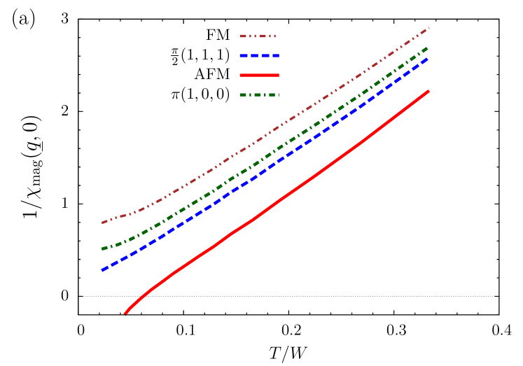
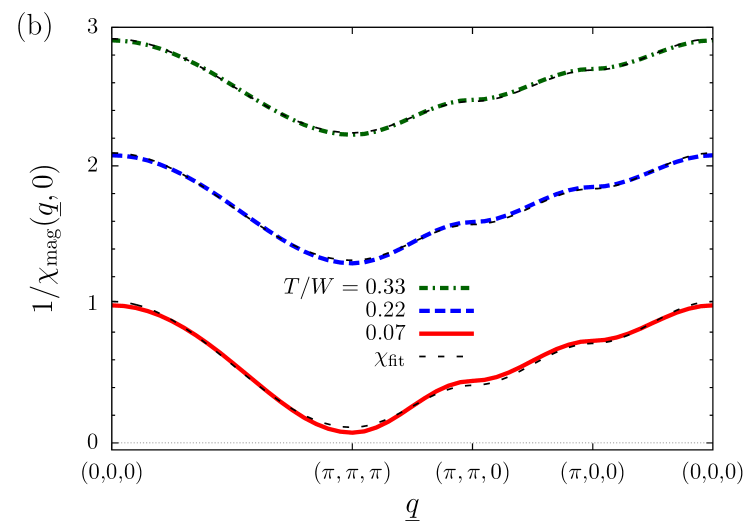
Figure 1: (Color online) Inverse static susceptibility (a) as function of temperature for various values of the wave vector ${\underline{q}}$ and (b) as function of ${\underline{q}}$ for three different temperatures. Both plots are calculated for the SC lattice with nearest neighbor hopping only ($t^{\prime}=0$), $U/W=1.5$, and at half-filling $n=1$.

Figure 1(a) displays the temperature dependent inverse static susceptibility for a half-filled SC lattice in three dimensions and various wave vectors ${\underline{q}}$. $\chi_{\mathrm{mag}}({\underline{q}},\nu=0)^{-1}$ depends almost linearly on $T$ over the whole range of temperatures, which is expected from the mean-field character of DMFT.Jarrell (1992); Ulmke (1998); Byczuk and Vollhardt (2002) The wave-vector dependence of $\chi_{\mathrm{mag}}({\underline{q}},\nu=0)^{-1}$ is shown in Fig. 1(b) for various temperatures. The ${\underline{Q}}=\pi(1,1,1)^{T}$ component of the susceptibility is always largest, indicating the strong tendency toward AFM. The dashed lines are fits to an expansion of the inverse susceptibility up to second order in the hopping,

$$\chi_{\mathrm{fit}}({\underline{q}},\nu=0) =\frac{1}{a(T)+b(T)\langle t^{2}\rangle_{{\underline{q}}}}$$ (26)

where $\langle t^{2}\rangle_{{\underline{q}}}=\frac{1}{N}\sum_{{\underline{k}}}t_{{\underline{k}}+{\underline{q}}}t_{{\underline{k}}}$. For the simple-, body-centered, and face-centered cubic lattice with nearest and next-nearest neighbor hopping, $t$ and $t^{\prime}$ respectively, this elementary two-particle dispersion is just given by the negative single-particle dispersion, where all hopping-matrix elements are replaced with their squares,

$$\langle t^{2}\rangle_{{\underline{q}}} =-t_{{\underline{q}}}\big{|}_{t\to t^{2},t^{\prime}\to{t^{\prime}}^{2}}.$$ (27)

(The sign stems from the definition of the single-particle dispersion with an overall negative sign, see Eq. (25.)) This form approximates the ${\underline{q}}$-dependence of the actual susceptibility very well, as it is visible in Fig. 1(b).

This result provides a justification of the RPA-like decoupling of frequency sums in the Bethe-Salpeter equations. The reasoning is as follows: Comparing the ${\underline{q}}$-dependency of the approximate form Eq. (26) to Eq. (17), we can infer that the particle-hole propagator – as the only ${\underline{q}}$-dependent quantity entering the susceptibility – must be of the form

$$P({\underline{q}}) =\frac{p_{0}}{1-\alpha\langle t^{2}\rangle_{{\underline{q}}}}=p_{0}\sum_{n=0}^{\infty}\big{[}\alpha\langle t^{2}\rangle_{{\underline{q}}}\big{]}^{n}.$$ (28)

The geometric series, used in the last equality, can be interpreted as the result of an RPA-like decoupling of the frequency sums appearing in the expansion of the exact particle-hole propagator, see Eq. (51). Given the quality of the fit, we are led to the conclusion that the RPA-like decoupling works very well for the particle-hole propagator. It therefore seems reasonable to assume that it is also a good approximation in the Bethe-Salpeter equations.

The physical reason lies in the nature of antiferromagnetic correlations. They favor neighboring spins to point in opposite directions, which does not require a precise adjustment in the time-domain for a propagating particle-hole pair. Therefore, decoupling in frequency space cannot induce a qualitative error (in contrast to the ferromagnetic case, see below). We always found good agreement between the form of Eq. (26) and the calculated susceptibility, whenever the tendency toward AFM was dominant.

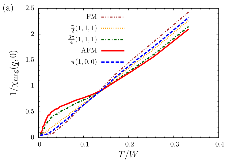
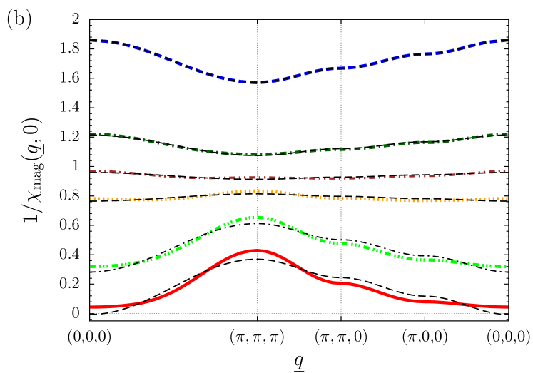
Figure 2: (Color online) (a) Inverse static susceptibility as function of temperature for various values of the wave vector ${\underline{q}}$. (b) $1/\chi_{\mathrm{mag}}({\underline{q}},0)$ as function of ${\underline{q}}$ for the temperatures (top to bottom): $T/W=0.26$, $0.17$, $0.14$, $0.12$, $0.065$, and $0.021$. Both plots are calculated for the SC lattice with nearest neighbor hopping only ($t^{\prime}=0$), $U/W=3.3$, and $n=0.97$.

For a larger Coulomb interaction of $U=3.3W$ and at finite doping, $\delta=3\%$ ($n=0.97$), the AFM susceptibility is largest only at high temperatures. This can be observed in Fig. 2(a) where $\chi({\underline{q}},0)^{-1}$ decreases linearly with temperature only for $T/W\gtrsim 0.2$ and changes qualitatively at low $T$. There, the FM component becomes dominant. The wave-vector dependency as shown in Fig. 2(b) is well approximated by Eq. (26) for the AFM-dominated region at high $T$, but below $T\lesssim 0.12W$ the fit does not work well and strong deviations occur.

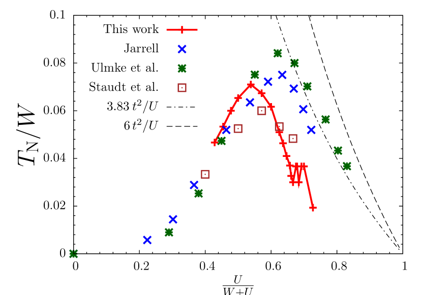
Figure 3: (Color online) The Néel temperature of the half-filled Hubbard model for the three dimensional SC lattice as function of $U$ (red line with points). For comparison, results from other studies are included as well: DMFT+QMCJarrell (1992) (blue crosses, labeled Jarrell), DMFT+QMCUlmke et al. (1995) (green stars, labeled Ulmke et al.), QMCStaudt et al. (2000) (brown squares, labeled Staudt et al.), high temperature expansionRushbrooke et al. (1974) (dash-dotted line, labeled $3.83t^{2}/U$), and mean-field (dashed-line, labeled $6t^{2}/U$).

The AFM transition temperature $T_{\mathrm{N}}$ (Néel temperature) is shown in Fig. 3 as function of the Coulomb repulsion for the half-filled ($\delta=0$) model. Results from other studies are also shown for comparison. The present result should be close to the data of Jarrell (Ref. Jarrell, 1992) or Ulmke et al. (Ref. Ulmke et al., 1995) as these results were also obtained with DMFT, but for a Gaussian (Jarrell) and semi-circular (Ulmke et al.) free DOS. For $U\leq W$ the agreement is quite satisfactory, while for larger $U$ the Néel temperature from the present approach is substantially smaller. It is, however, roughly in agreement with data from QMC simulations of the three-dimensional model (Staudt et al., Ref. Staudt et al., 2000) but this may be viewed as a coincidence.

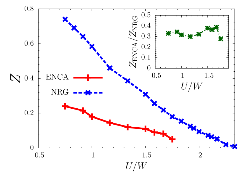
Figure 4: (Color online) The quasiparticle weight for the half-filled Hubbard model as function of the Coulomb repulsion $U$ extracted from the DMFT with ENCA and NRG as impurity solvers. The inset shows the ratio of both.

The exchange interaction decreases as $1/U$ in leading perturbative order for large $U$. Moreover, it is renormalized by small quasiparticle weights ($Z$-factors) when quasiparticle bands emerge. So a decrease of $T_{\mathrm{N}}$ at larger $U$ is to be expected, and its steepness depends on the size of the $Z$-factors,

$$Z =\frac{1}{1-\frac{\partial\mathrm{Re}\Sigma}{\partial\omega}(0)}.$$ (29)

While the ENCA as our impurity solver gives the correct order of magnitude and parameter dependence for the low-energy scale of the SIAM, it underestimates its actual value.Pruschke and Grewe (1989); *schmittSus09; *greweCA108 Within the self-consistent treatment of DMFT this tendency is retainedGrete et al. (2011) as it can be observed in Fig. 4 where $Z$ is shown as function of $U$. For comparison, the result from DMFT calculations with the NRGPeters et al. (2006) as impurity solver for the same parameter values is also shown. While the ENCA quasiparticle weight is smaller than the one extracted from the NRG, both follow the same trend. The inset displays the ratio of both and reveals the ENCA to yield a low-energy scale which is roughly a factor of $3$ too small. One may argue, that the ENCA-calculation is performed for an effectively larger value of the interaction $U$. Therefore, the reduction of the critical temperature compared to the other DMFT calculations as observed in Fig. 3 is a result of the too small low-energy scale of the ENCA.

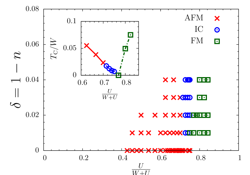
Figure 5: (Color online) Magnetic phase diagram in the $\delta$-$U$ plane. Each point indicates a magnetic phase transition. (The regions without points were unaccessible with the ENCA as impurity solver). The inset shows the transition temperature as function of $U$ for a fixed doping of $\delta=1-n=0.03$. In both graphs, the red crosses indicate AFM, the blue circles IC, and the green squares FM transitions.

Figure 5 displays the regions in the $\delta-U$ phase-space where magnetic phase transitions are observed. The AFM region extends from half-filling $\delta=0$ to finite doping for Coulomb interactions $U\lesssim 2.3W$ ($U/(W+U)\lesssim 0.7$). The investigation of regions in phase space with larger doping or smaller Coulomb repulsion was not possible, as there the pathology of the ENCAGrewe (1983); *kuramoto:AnalyticsNCA85; *Kuramoto:ncaIII84; *muellerhartmann:NCAgroundstate84; Pruschke and Grewe (1989); *schmittSus09; *greweCA108 prevented the access of low-enough temperatures.

In accord with earlier studiesPenn (1966); Freericks and Jarrell (1995); *tahvildar-zadeh3dHM97; *petersBetheHM09; Igoshev et al. (2010); Kuneš (2011) we also find incommensurate (IC) spin-density wave transitions away from half filling at the edge of the AFM region. As a function of $U$ (see inset) or doping (not shown), the transition temperature follows the trend foreshadowed by the Néel temperature, but the ordering vector shifts away from the AFM ${\underline{Q}}=\pi(1,1,1)^{T}$.Freericks and Jarrell (1995); *tahvildar-zadeh3dHM97; *petersBetheHM09

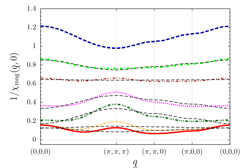
Figure 6: (Color online) Inverse static susceptibility as function of wave vector ${\underline{q}}$ for various values of temperature (top to bottom): $T/W=0.17$, $0.12$, $0.093$, $0.056$, $0.033$, $0.016$, and $0.012$. The curves are calculated for the SC lattice with nearest neighbor hopping only ($t^{\prime}=0$), $U/W=3$, and $n=0.97$.

This can be observed in Fig 6, where the inverse magnetic susceptibility is shown as function of ${\underline{q}}$ for various temperatures. There the transition vector probably lies in the region around ${\underline{q}}=(1,1,0)^{T}\pi$ but a precise location is not possible since we did not scan a sufficient part of the Brillouin zone but only along selected axes.

For finite doping, the nesting property of the Fermi surface is lost and incommensurate ordering is expected with increasing doping.Freericks and Jarrell (1995); *tahvildar-zadeh3dHM97; *petersBetheHM09 At a fixed doping, as presented in the inset of Fig. 5, the transition is induced by increasing the interaction. We attribute this to the temperature dependent formation of quasiparticles, whose characteristic energy scale is larger at lower $U$. There, the transition takes place at higher $T$ where the details of the Fermi surface are washed out and the nesting is approximately better fulfilled which leads to a AFM transition. Increasing $U$ decreases the transition temperature and the details of the Fermi surface become increasingly, making the system more sensitive to the lack of nesting and leading to the IC transition.

As depicted in the inset of Fig. 5, the AFM and FM phases seem to be separated by a quantum critical point (QCP), where the transition temperature vanishes and the systems goes from AFM to FM ground states at $T=0$. This QCP could in principle be physical as was speculated in the literatureZitzler et al. (2002) but this question can not be addressed within the present study. The ENCA as impurity solver does not allow the investigation of very low temperatures and consequently whether or not the transition temperature vanishes cannot be decided. As FM is overestimated within the present approach (see below) it could well be shifted to larger values of $U$ in more accurate treatments and thus removing the apparent QCP.

At very large $U\gtrsim 3W$ we observe FM at finite doping, which is the region where it is in principle expected and observed for various lattices.Ulmke (1998); Nagaoka (1965); *obermeierPruschke:FMHM97; *fazekasHM89; *merino:FMtriangular06; *petersFrustHM09; *guentherFMHM10 However, for the unfrustrated ($t^{\prime}=0$) SC lattice studied here, the transition temperatures $T_{\mathrm{C}}$ are too large (see inset).

We attribute this overestimation of the tendency toward FM to the RPA-like decoupling. Time-coherent propagation of particle-hole pairs over long distances is known to play a major role for FMHanisch et al. (1997); *hanisch:InstFMHM95; *hanisch:FerroHubbard (ordering vector ${\underline{Q}}=0$). FM correlations favor equal spin-alignment, and a transfer of electrons between sites does require a time-correlation with accompanying holes due to the Pauli principle. But such correlations in the time domain are not conserved by the RPA-frequency decoupling at interaction vertices. This conclusion is supported by the fact, that the FM transition temperatures as shown in the inset are roughly in accord with the Stoner-like criterion, $\rho(0,T_{\mathrm{C}})U\stackrel{{\scriptstyle!}}{{=}}1$, where $\rho(0,T)$ is the fully interacting and temperature dependent DOS at the Fermi level.

We have now established that the present approach yields reliable results whenever short-ranged particle-hole excitations dominate the magnetic response. In and close to the AFM regime, the transition temperatures are even reproduced quantitatively, apart from a reduction of $T_{\mathrm{N}}$ due to the too small low-energy scale produced by the ENCA. For very large Coulomb repulsions, the tendency towards FM is found to be overestimated which is attributed to the RPA-like decoupling of frequency sums in the Bethe-Salpeter equations.

III.2 Body-centered cubic lattice

In this section we focus on the three-dimensional body-centered cubic (BCC) lattice with nearest and next-nearest neighbor hopping, $t$ and $t^{\prime}$, respectively. The dispersion is given by

$$t_{{\underline{k}}}= -8t\cos(k_{x})\cos(k_{y})\cos(k_{z})$$ (30)

$$-2t^{\prime}\big{(}\cos(2k_{x})+\cos(2k_{y})+\cos(2k_{z})\big{)},$$

where the half bandwidth is $W=8t$ as long as $|t^{\prime}|\leq\frac{4}{3}|t|$, which is always the case in the following. As for the SC lattice, the BCC lattice is bipartite and exhibits perfect nesting for vanishing next-nearest neighbor hopping, $t^{\prime}=0$. The AFM nesting vectors ${\underline{Q}}$ satisfy $t_{{\underline{k}}+{\underline{Q}}}=-t_{{\underline{k}}}$ and are of the type ${\underline{Q}}=\pi(1,0,0)^{T}$ and ${\underline{Q}}=\pi(1,1,1)^{T}$.

The perfect nesting property is illustrated in Fig. 7, where the Fermi surface of the noninteracting system at half-filling is shown for two values of the next-nearest neighbor hopping, $t^{\prime}=0$ and $t^{\prime}=-0.2t$. The flat and parallel sections of the Fermi surface are clearly visible for $t^{\prime}=0$ in panel (a). For finite $t^{\prime}$ (see panel (b)) the Fermi surface acquires a substantial curvature so that the nesting vector no longer connects large parts of the Fermi surface.

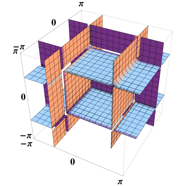
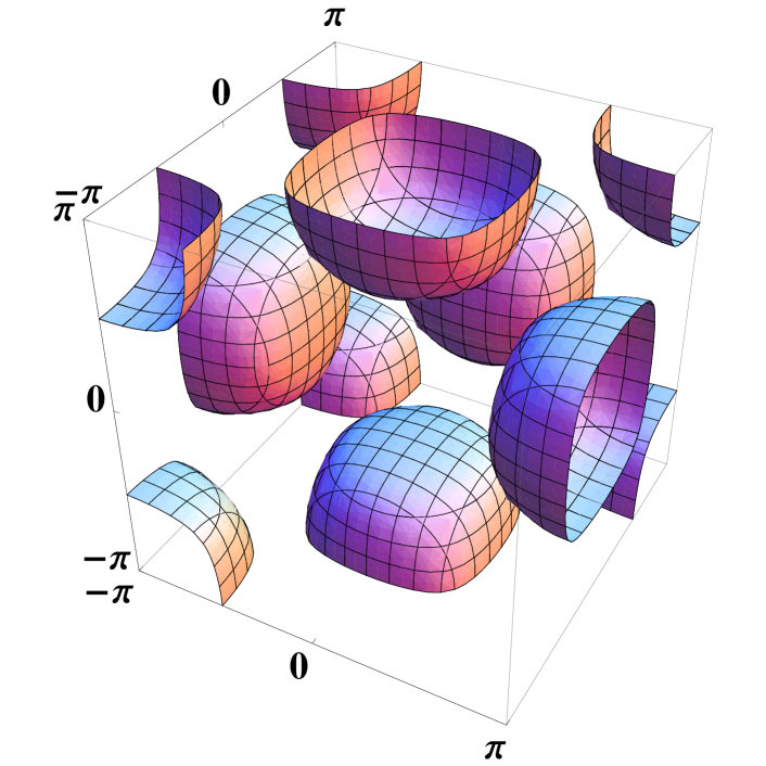
Figure 7: (Color online) Noninteracting Fermi surface for the BCC lattice for (a) $t^{\prime}=0$ and (b) $t^{\prime}=-0.2t$ at half-filling. (In the front quadrant some parts are omitted in order to get a better view.)

The noninteracting DOS as shown in Fig. 8 displays the characteristic van-Hove singularities due to the extrema and saddle points of the dispersion relation $t_{\underline{k}}$ in the Brillouin zone. Most prominent is the logarithmic divergence near the Fermi level due to the maxima at ${\underline{k}}=\frac{\pi}{2}(1,0,0)^{T}$. Such a van-Hove singularity can induce profound changes in the low temperature, low-energy Fermi liquid properties, even in DMFT.Schmitt (2010) But here we do not study this possibility but focus on magnetic transitions which generally occur at higher temperatures.

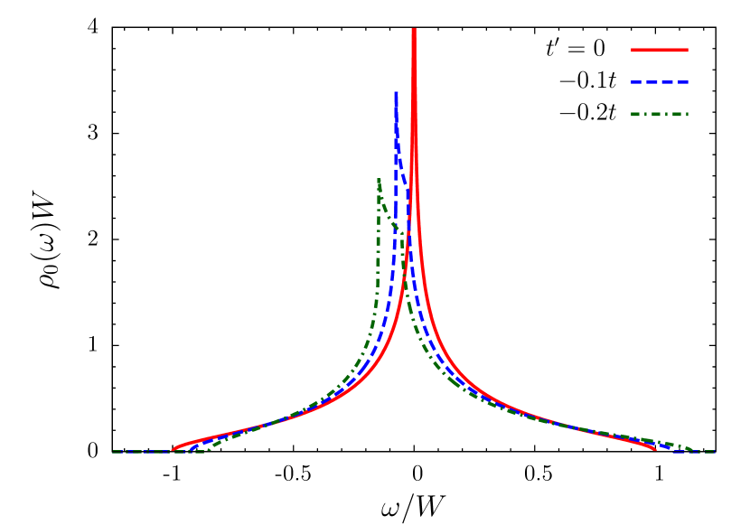
Figure 8: (Color online) Noninteracting DOS for the BCC lattice at half-filling and three different next-nearest neighbor hoppings, $t^{\prime}/t=0$, $-0.1$, and $-0.2$.

The reason we are considering the BCC lattice instead of the more common SC lattice is found in the more pronounced influence of the frustrating next-nearest neighbor hopping $t^{\prime}$ in the former lattice. The shape of the Fermi surface changes much more strongly with increasing $t^{\prime}$ for the BCC lattice as, for example, in the SC lattice. In particular, results pointing to a competition between local-moment and quasiparticle magnetism are found to be more pronounced for the BCC lattice than for the SC case, even though we also observed them in the latter case as well.

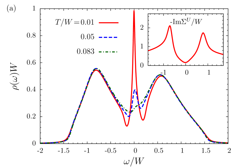
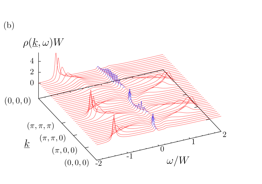
Figure 9: (Color online) (a) Local spectral function $\rho(\omega)$ obtained with the DMFT for the BCC lattice for three different temperatures. The curves are calculated for half-filling with a Coulomb interaction $U/W=1.375$ and a finite next-nearest neighbor hopping $t^{\prime}/t=-0.2$ is used. The inset shows the (negative) imaginary part of the self-energy -Im$\Sigma(\omega+i\delta)$ for the lowest temperature $T/W=0.01$. (b) The momentum dependent lattice spectral function as function of ${\underline{k}}$ along high symmetry directions in the Brillouin zone for the same parameters as in (a) and $T/W=0.01$.

A DMFT-spectral function for the BCC lattice with finite next-nearest neighbor hopping is shown in Fig. 9. As a consequence of the rather large Coulomb interaction the lower and upper Hubbard band are clearly visible. Upon lowering the temperature a quasiparticle peak emerges at the Fermi level indicating the formation of a correlated metallic state. The inset shows the imaginary part of the self-energy. The quadratic minimum at the Fermi level reveals this state to be a Fermi liquid as it is expected within DMFT.Pruschke et al. (1995); *georges:dmft96; *georgesDMFTreview04; Müller-Hartmann (1989b); Schmitt (2010) The momentum resolved spectral function $\rho({\underline{k}},\omega)$ shown in panel (b) exhibits the dispersive low-energy quasiparticle band around the Fermi level.

The formation of this low-temperature Fermi liquid is associated with a screening of local magnetic moments due to Kondo-correlations.

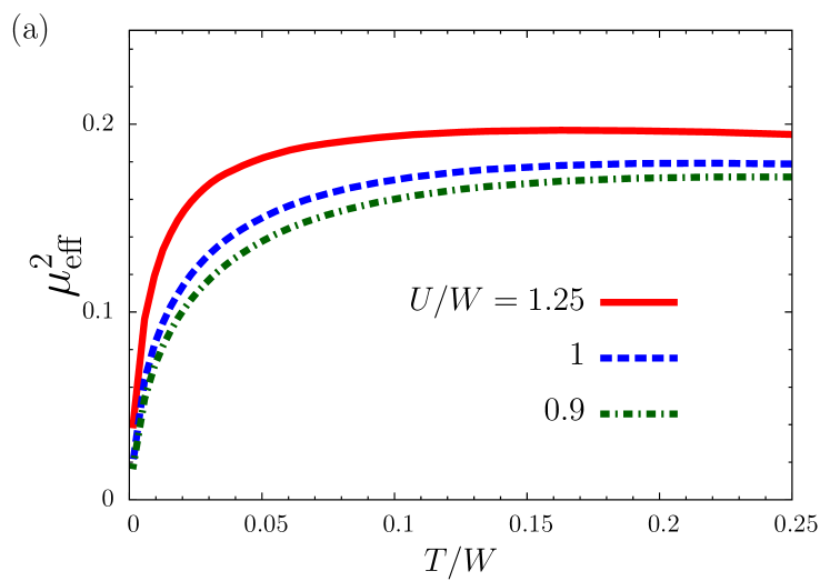
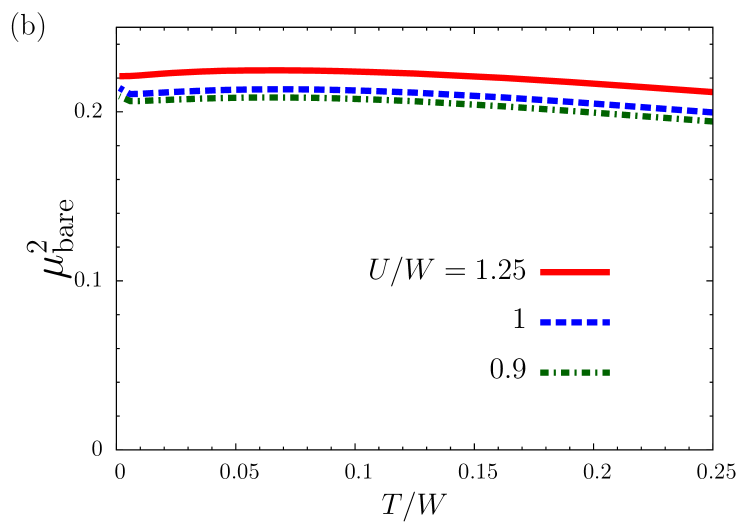
Figure 10: (Color online) The screened (a) and unscreened (b) local moment, $\mu_{\text{eff}}^{2}$ and $\mu_{\text{bare}}^{2}$, respectively, as function of temperature for $t^{\prime}/t=-0.15$ and three different values of the Coulomb interaction.

Figure 10(a) displays the screened local moment,

$$\mu_{\text{eff}}^{2}=T\chi^{\mathrm{loc}}_{\mathrm{mag}}(T),$$ (31)

as function of temperature for three different values of the Coulomb interactions. Due to the Coulomb interaction the moments at high temperatures are larger than the induced moment $\mu_{\text{eff},U=0}^{2}=\frac{1}{8}$ of the noninteracting band electrons (where empty and doubly occupied local states fully contribute), and increases with $U$ toward the value $\mu_{\text{eff},\mathrm{spin}}^{2}=\frac{1}{4}$ of a free spin. At temperatures of the order of the characteristic low-energy scale $T^{*}=WZ$, where $Z$ is the quasiparticle weight of Eq. (29), the moments decrease due to the buildup of Kondo-correlations.

In contrast, the unscreened moment

$$\mu_{\text{bare}}^{2}=\frac{1}{4}\big{[}\langle\hat{n}_{\uparrow}\rangle+\langle\hat{n}_{\downarrow}\rangle-2\langle\hat{n}_{\uparrow}\hat{n}_{\downarrow}\rangle\big{]}$$ (32)

which is essentially determined by the double occupancy is almost independent of temperature, see Fig. 10(b). Upon lowering the temperature it slightly increases due to the decrease in the thermally induced double occupancy. The formation of the Fermi liquid quasiparticle band at low temperatures then leads to a slight increase of the double occupancyGeorges and Krauth (1993); Daré and Albinet (2000) and consequently the moment decreases again.

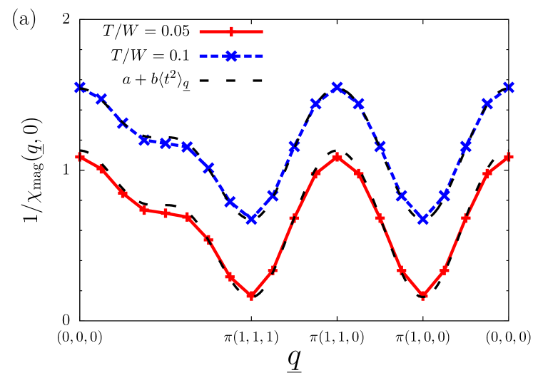
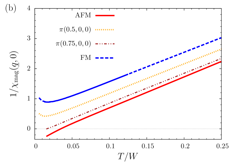
Figure 11: (Color online) (a) The inverse magnetic susceptibility for different temperatures as function of the wave vector along with fits of the form $a+b\langle t^{2}\rangle_{\underline{q}}$, see Eq. (26). (b) The inverse magnetic susceptibility for different wave vectors as function of temperature. The curves are calculated for half-filling with a Coulomb interaction $U/W=1.25$ and a next-nearest neighbor hopping of $t^{\prime}/t=-0.15$.

AFM should prevail for not too large next-nearest neighbor hopping $t^{\prime}$ due to the near-nesting property of the Fermi surface. Figure 11(a) displays the inverse magnetic susceptibility for $U/W=1.25$ and $t^{\prime}/t=-0.15$ as function of the wave vector along a path through the Brillouin zone. As in the previous section for the SC lattice, the AFM components (${\underline{Q}}=\pi(1,0,0)^{T}$ and ${\underline{Q}}=\pi(1,1,1)^{T}$) are enhanced. Additionally, fits with the approximate function of Eq. (26) agree very well with the susceptibility, supporting the view developed in the previous section. The temperature dependence of the susceptibility is depicted in Fig. 11(b). The AFM component exhibits a Curie-Weiss behavior $\frac{1}{T-T_{\mathrm{N}}}$ with a divergence at $T_{\mathrm{N}}/W\approx 0.035$, which supports an interpretation in terms of local-moment magnetism.

However, this perspective becomes less obvious when the constituents are analyzed in detail. The effective local moment which enters Eq. (17a) is temperature dependent due to screening, see Fig. 10. Additionally, the static exchange coupling $J({\underline{q}},\nu=0)$ also displays a temperature dependency. This can be observed in Fig. 12(a), where the AFM coupling $J({\underline{Q}},0)$ slightly increases toward lower temperatures. The increase in $J({\underline{Q}},0)$ is compensated by the reduced moment and together both yield the observed Curie-Weiss behavior characteristic of local-moment magnetism.

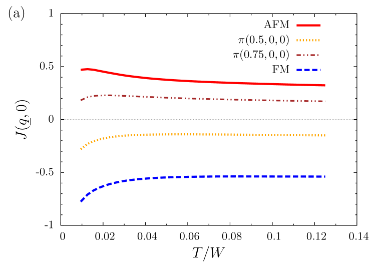
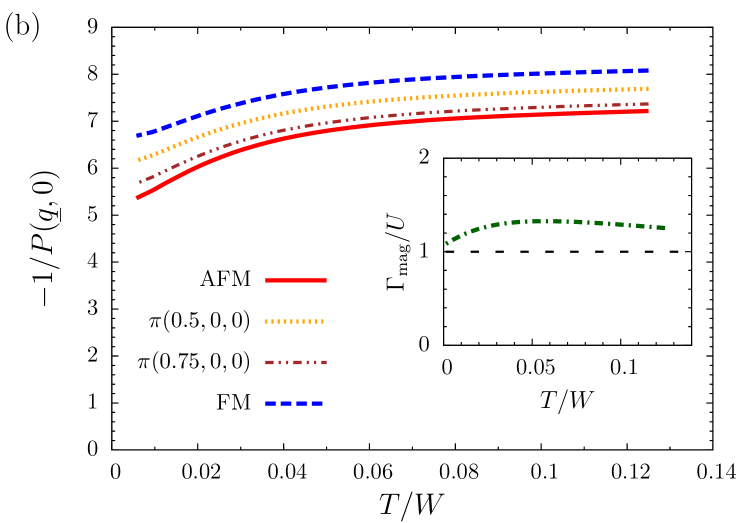
Figure 12: (Color online) (a) The effective static exchange coupling $J({\underline{q}},\nu=0)$ of Eq. (18) for different wave vectors as function of temperature for $U/W=1.25$ and $t^{\prime}/t=-0.15$. (b) The inverse negative static particle-hole propagator for different wave vectors as function of temperature. The inset displays the effective local vertex of Eq. (22).

Figure 12(b) shows the same data but organized in terms of the itinerant picture of magnetism. The “noninteracting” susceptibility, i.e. the particle-hole propagator calculated without explicit two-particle interactions but with the full single-particle Green functions, increases with decreasing temperature for all wave vectors. This is a consequence of the accumulation of spectral weight near the Fermi level, cf. Fig. 9(a). The effective magnetic two-particle vertex $\Gamma_{\mathrm{mag}}(\nu=0)$ is of the order but slightly larger then the bare interaction $U$ (see inset). It slightly decreases for low temperatures indicating the quasiparticle excitations to experience somewhat less scattering.

Thus, the buildup of Kondo-like resonances in the lattice has two opposing effects, which nearly compensate each other here: The screening of local moments and the accumulation of additional quasiparticle weight near the Fermi level.

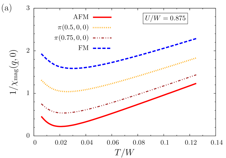
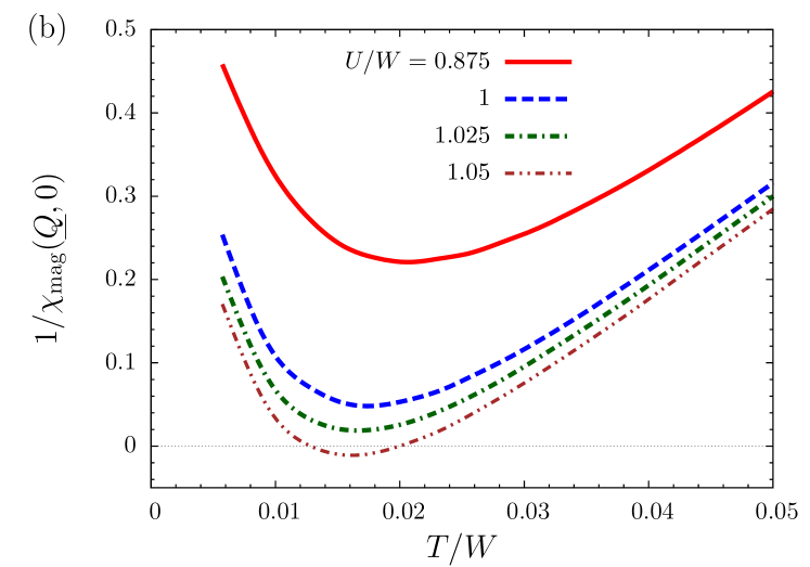
Figure 13: (Color online) (a) The inverse magnetic susceptibility for different wave vectors as function of temperature for $U/W=0.875$. (b) The inverse AFM component of the susceptibility for small temperatures and various values of $U$. In both plots is $t^{\prime}/t=-0.17$.

The balance between itinerant and localized contributions to the susceptibility is rather fragile. Already for moderate changes of parameter values the Curie-Weiss behavior of the susceptibility is lost. This is the case for a slightly larger next-nearest neighbor hopping of $t^{\prime}/t=-0.17$ and $U/W=0.875$ as shown in Fig. 13(a). AFM is still dominant but no magnetic transition occurs. All components of the susceptibility exhibit a maximum (minimum in inverse susceptibility) and decrease toward lower temperatures. The decrease occurs at a temperature of the order of the low-energy scale indicating that the coherent quasiparticles do not favor any tendency toward magnetic order.

This maximum in the susceptibility opens up the possibility of an unusual phase-transition scenario. Increasing the Coulomb repulsion enhances the AFM susceptibility as can be seen in Fig. 13(b). For large enough $U$, the minimum in $1/{\chi_{\mathrm{mag}}({\underline{Q}},0)}$ even reaches zero indicating a divergent susceptibility at a finite temperature ($T_{\mathrm{N}}/W\approx 0.016$ for the case shown in the graph with a Coulomb repulsion between $U/W=1.025$ and $U/W=1.05$).

Fixing the temperature at some value and increasing $U$ can lead to the peculiar situation that the system stays paramagnetic even though at a higher temperature it would undergo an AFM phase-transition. In that regime, there exists a finite temperature interval $T_{\mathrm{N,1}}\leq T\leq T_{\mathrm{N,2}}$ in which AFM order is expected to occur, while outside this interval the system stays paramagnetic. Unusually, for $T<T_{\mathrm{N},1}$ the system can be driven into the AFM ordered phase by heating it.

It should be noted, that similar re-entrant behavior was already found for the AFM transition in the Hubbard model within a weak-coupling treatment for an infinite- and two- dimensional lattice,Halvorsen and Czycholl (1994); Hong et al. (1996) as well as within an equation of motion technique.Mancini and Avella (2004) In these cases, the frustration was brought about by finite hole-doping, instead of a finite next-nearest neighbor hopping implemented here. The extended Hubbard model with an additional nearest-neighbor Coulomb interaction also displays a re-entrant behavior for the charge-ordering transition.Pietig et al. (1999)

Another peculiarity feature is connected to the critical exponent. The theory we employed has mean-field character regarding spatial correlations. Thus, we expect a mean-field critical exponent $\gamma=1$ for the nonlocal magnetic susceptibility, $\chi({\underline{Q}},T)\sim(T-T_{C})^{-\gamma}$. This exponent is indeed always found, except for that value of $U$ where the minimum in $\chi^{-1}$ touches the zero-axis. There, the exponent is is larger and of the order $\gamma=2$ as this minimum can be fit with a parabola.

The re-entrant behavior is a result of the competition between the ordering of local moments and the formation of low-temperature quasiparticles, i.e. the competition between local moment and itinerant quasiparticle magnetism. The exact shape of the Fermi surface has a strong influence on the quasiparticle scattering which determines the particle-hole propagator. At low temperatures, the quasiparticles are fully formed and the frustration induced by $t^{\prime}$ leads to a suppression of the particle-hole propagator, essentially eliminating magnetism (similar to what happens at weak coupling).

This can be observed in Fig. 14(a), where the inverse particle-hole propagator shows a saturation and even a slight upturn toward low temperatures (compare Fig. 12(b) where this is not the case), even though the system is metallic with large spectral weight at the Fermi level, cf. Fig. 9(a). The effective vertex (see inset) is not sensitive to the Fermi surface and consequently displays a qualitatively similar behavior to the case shown in Fig. 12(b).

A local moment perspective can be employed above $T/W\approx 0.02$ where the effective exchange coupling $J$ is almost temperature independent (see Fig. 14(b)) and very similar to the one shown in Fig. 12(a). Below this temperature, however, coherent quasiparticles emerge and the coupling changes dramatically. The AFM component even changes sign and becomes ferromagnetic.

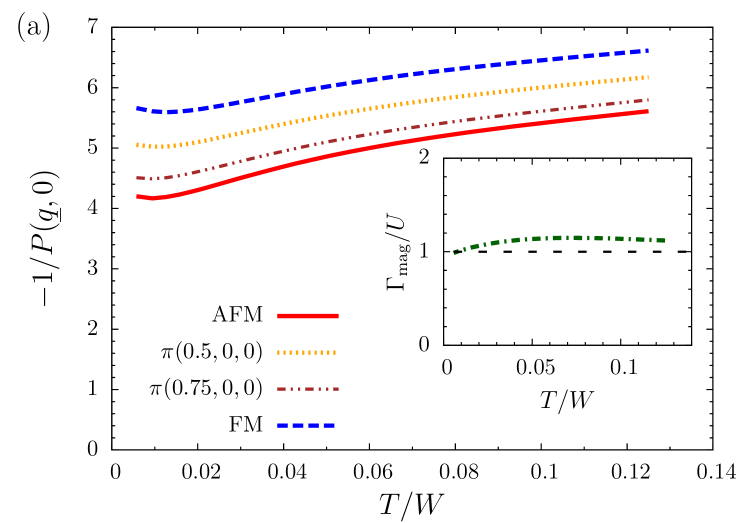
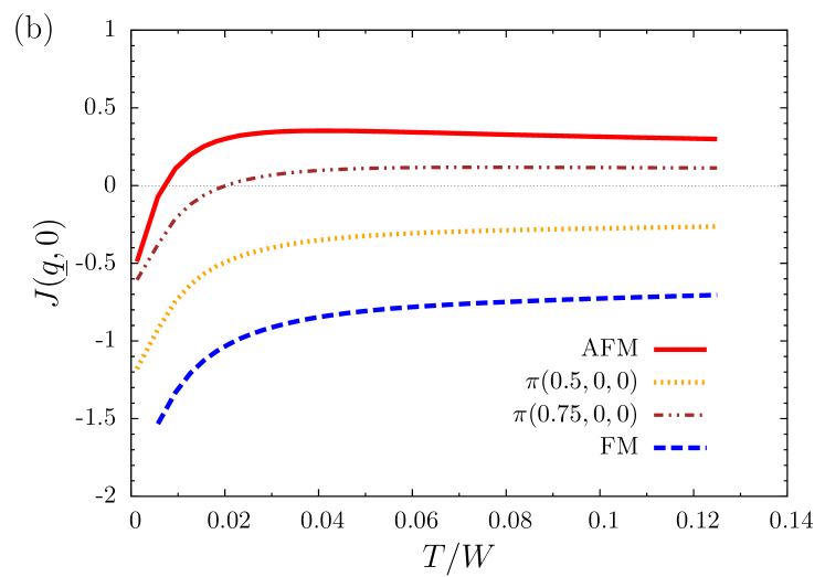
Figure 14: (Color online) (a) The inverse negative static particle-hole propagator for different wave vectors as function of temperature. The inset displays the effective local vertex of Eq. (22). (b) The effective static exchange coupling $J({\underline{q}},\nu=0)$ of Eq. (18) for different wave vectors as function of temperature. for In both plots $U/W=1$ and $t^{\prime}/t=-0.17$ is used.

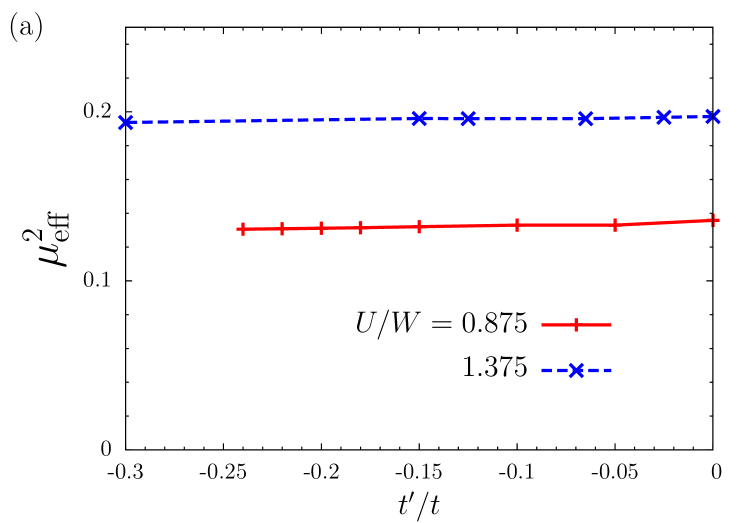
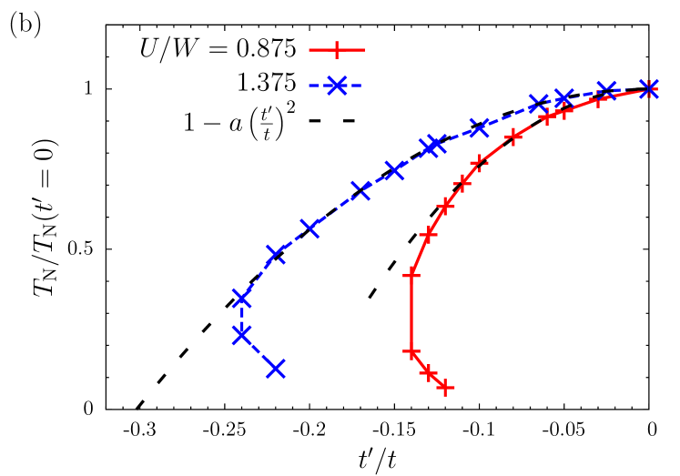
Figure 15: (Color online) (a) The effective local moment as function of the next-nearest neighbor hopping $t^{\prime}$ for a fixed temperature $T/W=0.046$ and two values of the Coulomb repulsion. (b) The Néel temperature as function of $t^{\prime}$ normalized to its value for $t^{\prime}=0$ for two values of $U$. Also shown are fits with a quadratic decrease, where the fit parameters are $a=24$ and $a=10.95$ for $U/W=0.875$ and $U/W=1.375$, respectively.

Whether the local moments order at higher temperature is determined by their size and the geometry of the lattice. Both aspects are much less sensitive to the frustration generated by a finite $t^{\prime}$ than the magnetic quasiparticle scattering. The value of the screened effective moments is not influenced much by $t^{\prime}$ as can be seen in Fig. 15(a). $\mu_{\mathrm{eff}}^{2}$ is shown for a fixed temperature as function of $t^{\prime}$ for two different values of $U$. The decrease with increasing $t^{\prime}$ is barely visible confirming the screening to be independent of the details of the Fermi surface or the shape of the spectral functions (as long as the system is a metal, of course).

In order to get an estimate for the $t^{\prime}$ dependence of the Néel temperature from the local moment perspective, it is instructive to start from the atomic limit. The effective exchange coupling can be estimated in second order perturbation theory in the hopping,

$$J_{\mathrm{eff}}({\underline{q}}) =-\frac{8t^{2}}{U}\cos(q_{x})\cos(q_{y})\cos(q_{z})$$ (33)

$$-\frac{2{t^{\prime}}^{2}}{U}\Big{[}\cos(2q_{x})+\cos(2q_{y})+\cos(2q_{z})\Big{]},$$

which yields the effective AFM coupling for ${\underline{q}}={\underline{Q}}$,

$$J_{\mathrm{eff}}^{\mathrm{AFM}} =\frac{8t^{2}}{U}\Big{(}1-\frac{3}{4}\frac{{t^{\prime}}^{2}}{t^{2}}\Big{)}\equiv J_{t^{\prime}=0}^{\mathrm{AFM}}\Big{(}1-\frac{3}{4}\frac{{t^{\prime}}^{2}}{t^{2}}\Big{)}.$$ (34)

This coupling directly determines the AFM transition temperature as it was discusses around Eq. (21). The Hubbard model for the parameter values under consideration is far from the atomic limit as it is a metal and itinerant electronic excitations are present. However, for the local moment picture to be applicable the Néel temperature should follow the quadratic decrease with $t^{\prime}$ of Eq. (34), but renormalized pre-factors would be expected. Figure 15(b) displays $T_{\mathrm{N}}$ as function of $t^{\prime}$ for two different values of $U$. The transition temperature indeed decreases in accordance with that expectation for small to moderate values of $|t^{\prime}/t|$. The rather large values for the fit parameter $a$ compared to $3/4$ of Eq. (34) indicate strong renormalizations due to the formation of heavy quasiparticles. At too large $t^{\prime}$, the Néel temperature comes in regions where the forming quasiparticles begin to dominate and magnetism is suppressed quite abruptly. For smaller values of $U$, the local moments are generally less pronounced and consequently this suppression occurs faster.

The Néel temperature does not go to zero continuously, but rather remains finite at the maximal $t^{\prime}$ where a transition occurs. In the vicinity of this value the re-entrant behavior can be observed, and the system tends to exhibit AFM only in a finite temperature interval.

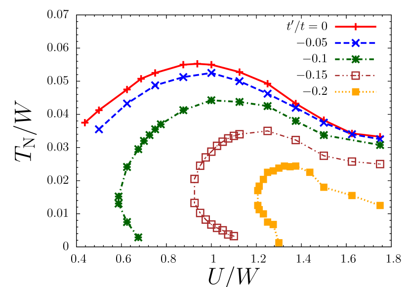
Figure 16: (Color online) The Néel temperature of the half-filled Hubbard model on BCC lattice as function of $U$ for various $t^{\prime}$.

The Néel temperature as function of the Coulomb repulsion $U$ for various values of the next-nearest neighbor hopping $t^{\prime}$ is shown in Fig. 16. With increasing $t^{\prime}$ the transition temperature is generally reduced especially in the weak coupling regime where AFM is completely eliminated. For finite $t^{\prime}$, there exists a nonzero critical value for the Coulomb repulsion, $U_{\mathrm{C}}>0$, only above which AFM can occur. Similar behavior is found for the SC lattice with finite next-nearest neighbor hopping $t^{\prime}$.Zitzler et al. (2004) The perturbation expansion in $U$ shows that for vanishing next-nearest neighbor hopping, $t^{\prime}=0$, AFM extends to $U=0$, i.e. $U_{\mathrm{C}}=0$, due to perfect nesting (see, for example, Ref. Fazekas, 1999, Chap. 7).

For large $U$ AFM is found to be very robust with respect to $t^{\prime}$ and $T_{\mathrm{N}}$ is only reduced. The dependence of the Néel temperature on $t^{\prime}$ is in agreement with the quadratic decrease expected from a local-moment picture, and the quadratic coefficient of the $t^{\prime}$-term decreases with increasing $U$, cf. Fig 15(b). In the crossover regime at intermediate $U/W$ the re-entrant behavior is observed. For a given $U$, there exist two critical temperatures, $T_{\mathrm{N,2}}$ and $T_{\mathrm{N,1}}$, between which the system exhibits AFM, while below $T_{\mathrm{N,1}}$ and above $T_{\mathrm{N,2}}$ paramagnetism prevails.

IV Conclusion and Outlook

We have derived an universal and physically intuitive form of the magnetic susceptibility of strongly correlated electron systems within DMFT using an additional RPA-like decoupling in the Bethe-Salpeter equations. It was thus possible to work completely in the real-frequency domain and to write this final expression in terms of functions of real variables, which all are obtained from an effective impurity model. The static and dynamic magnetic response could readily be calculated from there.

We analyzed the validity of this form and found the RPA-like decoupling to be quantitatively correct whenever short-ranged particle-hole excitations dominate. This is the case in and close to the antiferromagnetic region in phase space of the Hubbard model where the Néel temperature was correctly reproduced (modulo shortcomings of the ENCA impurity solver).

The tendency toward ferromagnetism, on the other hand, is overestimated by the approach as a direct consequence of the decoupling. However, this shortcoming could be circumvented in the future by employing a different decoupling strategy, where averages are taken over products of a particle-hole propagator and a local vertex. Leading order coherence effects during a two-particle interaction should then be retained.

The applicability of the two archetypical pictures of magnetism was then investigated in case of the Hubbard model on a three-dimensional body-centered cubic lattice with next-nearest neighbor hopping. For small interactions strength the antiferromagnetism can be understood in terms of itinerant quasiparticles. The magnetic response is determined by particle-hole excitations across the Fermi surface. With increasing next-nearest neighbor hopping $t^{\prime}$, the perfect-nesting property of the Fermi surface is lost rapidly. As a consequence, AFM is almost entirely removed from the weak coupling phase diagram.

At large values of the local Coulomb interaction $U$ the local-moment picture is more appropriate, as the antiferromagnetism is rather robust against geometric frustration induced by $t^{\prime}$. The expansion around the atomic limit provides an suggestive form for the $t^{\prime}$-dependence of the Néel temperature which is in agreement with the DMFT results.

At intermediate $U$ both types of magnetism compete. The many-body effects leading to the formation of the quasiparticle bands and the screening of local moments are strongly temperature dependent. This produces an unusual re-entrant behavior. Local moments still sizable at elevated temperatures order antiferromagnetically at a characteristic temperature $T_{\mathrm{N},2}$. But at even lower temperatures the coherent quasiparticles are dominating and due to the lack of nesting of the Fermi surface, magnetism is suppressed below $T_{\mathrm{N},1}$.

Beyond the scope of magnetism, the interplay of localized and itinerant effective pictures is of fundamental interest. For example, the explanation of the re-entrant Mott-transition found in the highly frustrated organic compound $\kappa$-(ET)₂Cu[N(CN)₂]ClKagawa et al. (2004); *ohashiTriangularHM08; *ohashiTriangularHM08-2 is in direct analogy to the mechanism presented here. The temperature dependency of the effective picture and the re-entrant behavior is generated by a competition between frustrated magnetic moments and a low temperature Fermi liquid.

It is an interesting prospect and needs further investigations whether similar temperature dependencies could play a role in other strongly correlated systems. In the cuprate superconductors,Plakida (2010) for example, the single-particle excitations are believed to be of a more itinerant character along the nodal direction while of more localized nature along the anti-nodal.Shen and Davis (2008) The frustration brought about by the next-nearest neighbor hopping $t^{\prime}$ could play a decisive role, at least for some compounds and parameter values.

Appendix A DMFT for single particle Green functions

In this section we sketch the DMFT self-consistency which will turn out to be useful for the formulation of the two-particle properties in appendix B. The Dyson-equation can be written in terms of the effective local single-particle cumulant Green function

$$\tilde{G}(z)=\frac{1}{z-\Sigma^{U}(z)}.$$ (35)

This quantity represent dressed atomsMetzner (1991) between which single-particle transfers $t_{\underline{k}}$ are possible. This view is established within the linked cluster expansion around the atomic limit utilizing local cumulantsMetzner (1991); Grewe et al. (2008); Grewe (1996); Schmitt (2009) and yields the Dyson equation

$$G({\underline{k}},z) =\tilde{G}(z)+\tilde{G}(z)\>t_{\underline{k}}\>G({\underline{k}},z).$$ (36)

Solving this equation for the Green function just gives Eq. (4).

The local Green function is obtained by a Fourier transform

$$G(z) =\tilde{G}(z)+\tilde{G}(z)\frac{1}{N}\sum_{\underline{k}}t_{\underline{k}}\>G({\underline{k}},z)$$ (37)

$$=\tilde{G}(z)+\tilde{G}(z)\>T(z)\>\tilde{G}(z).$$ (38)

It was used that $\sum t_{\underline{k}}=0$, which holds for all inversion symmetric lattices and we introduced the local scattering matrix

$$T(z) =\frac{1}{N}\sum_{\underline{k}}t_{\underline{k}}\>G({\underline{k}},z)\>t_{\underline{k}}.$$ (39)

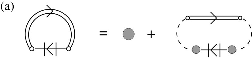
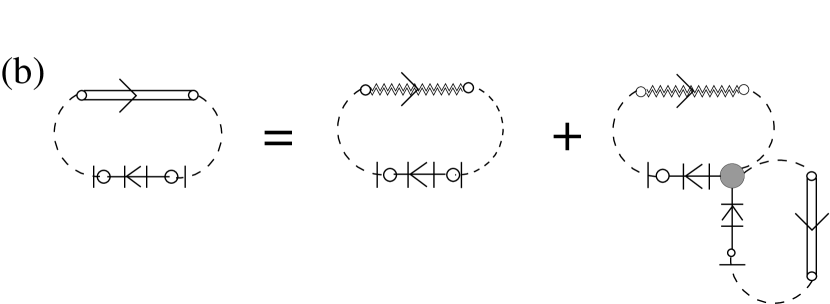
Figure 17: (a) Dyson equation for the local single-particle Green function in terms of the local cumulant $\tilde{G}$ (grey shaded circles) and the local scattering matrix $T(z)$. The double line with the arrow and the small circles at the end indicate a full Green functions $G({\underline{k}},z)$ and a dashed line an elementary hopping $t_{\underline{k}}$. (b) The local scattering matrix $T(z)$ in terms of the irreducible loops, i.e. the effective medium, $\Gamma(z)$ as in Eq. (42). The full scattering matrix is already graphically composed of two elementary hoppings and a full propagation, see Eq. (39). The effective medium is represented in a similar way, only the propagation through the lattice without visits to the local site is indicated by a zig-zag line. In both quantities the elementary hoppings are included and, therefore, do not appear in Eq. (40) - (42). The start and end points of all propagations are connected to indicate local i.e. ${\underline{k}}$-summed quantities and the small horizontal bars indicate that these lines are not accounted for in an analytical expression. The small circles are drawn only to indicate a lattice site at which a propagation starts/ends and do not appear in any analytical expressions. In the present context these are unnecessary, but they are helpful for two-particle quantities which are discussed in the next section.

A graphical representation of this equation is depicted in Fig. 17(a). $T(z)$ incorporates all processes where an electron leaves the site under consideration, propagates through the entire lattice —including that local site— and then returns. These processes can be reorganized in terms of re-visits to the local site,Craco and Gusmão (1995)

$$T(z) =\Gamma(z)+\Gamma(z)\>\tilde{G}(z)\>\Gamma(z)+\dots$$ (40)

$$=\Gamma(z)+\Gamma(z)\>\tilde{G}(z)\>T(z)$$ (41)

$$=\frac{1}{\Gamma(z)^{-1}-\tilde{G}(z)}.$$ (42)

The effective medium $\Gamma(z)$ now has the clear interpretation of being the irreducible loop for a propagation of an electron from a specific site through the lattice back to that site, without returning during the propagation, see Fig. 17(b). This makes it very obvious to interpreted $\Gamma$ as an noninteracting effective medium and thus establishes the DMFT mapping of the lattice problem to an SIAM.

Formally, this is obtained by inserting Eq. (42) into Eq. (38) which gives the local Green function

$$G(z) =\frac{1}{\tilde{G}^{-1}-\Gamma(z)}$$ (43)

which is nothing but Eq. (6).

Appendix B Bethe-Salpeter equations and dynamic susceptibilities

The physical susceptibility matrix depends on one external bosonic Matsubara frequency $i\nu_{n}$ and wave vector ${\underline{q}}$. It is obtained from a more general two-particle Green function by summing over two internal fermionic frequencies and wave vectors (omitting the convergence factors $e^{(i\omega_{1}\!+i\omega_{2})\delta}$),

$$\uuline{\chi}{}({\underline{q}},i\nu_{n}) =\frac{1}{\beta N}\sum_{i\omega_{1},i\omega_{2}}\sum_{{\underline{k}}_{1},{\underline{k}}_{2}}\uuline{\chi}{}({\underline{q}},i\nu_{n}|{\underline{k}}_{1},{\underline{k}}_{2}|i\omega_{1},i\omega_{2})$$ (44)

$$\equiv\frac{1}{\beta}\sum_{i\omega_{1},i\omega_{2}}\uuline{\chi}{}({\underline{q}},i\nu_{n}|i\omega_{1},i\omega_{2}).$$ (45)

Here, $i\omega_{1}$ and $i\omega_{2}$ are short-hand notations for the sets of fermionic Matsubara frequencies $i\omega_{n_{1}}$ and $i\omega_{n_{2}}$ ($n_{1},n_{2}\in\mathbb{Z}$). The notation is introduced to discriminate between external arguments ($i\nu_{n}$, ${\underline{q}}$) and internal momenta (${\underline{k}}_{1}$, ${\underline{k}}_{2}$) and frequencies ($i\omega_{1}$, $i\omega_{2}$) which are separated by vertical bars. In the last equation we absorbed the momentum sum into the susceptibility as indicated by the missing internal momentum variables.

We also introduced a matrix notation for two-particle quantities in orbital/spin space indicated by the straight double underline, i.e. $A_{a,b;c,d}=\{\uuline{A}{}\}_{a,b;c,d}$. The matrix multiplication is defined as

$$\{\uuline{A}{}\,\uuline{B}{}\}_{a,b;c,d} =\sum_{ef}A_{f,b;c,e}B_{a,e;f,d}.$$ (46)

Figure 18: Graphical representation of the susceptibility matrix $\chi_{a,b;b,a}({\underline{q}},i\nu_{n}|{\underline{k}}_{1},{\underline{k}}_{2}|i\omega_{1},i\omega_{2})$.

The graphical representation of the susceptibility matrix $\uuline{\chi}{}({\underline{q}},i\nu_{n}|{\underline{k}}_{1},{\underline{k}}_{2}|i\omega_{1},i\omega_{2})$ is shown in Fig. 18. The two external pairwise contracted lines signal the specific choice of orbital matrix elements $\chi_{a,b;b,a}$, as well as frequency and momentum arguments.

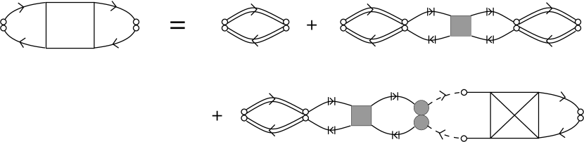
Figure 19: Bethe-Salpeter equation for the susceptibility matrix. The shaded square represents the irreducible vertex $\Pi$.

The Bethe-Salpeter equation for the susceptibility matrix is obtained by summing all particle-hole reducible diagrams not accounted for in the vertex $\uuline{\Pi}{}$. This is shown graphically in Fig. 19.

Within DMFT the full particle-hole irreducible two-particle vertex $\uuline{\Pi}{}$ is assumed to be momentum independent and momentum conservation is ignored at internal vertices. This allows all sums over internal momenta to be absorbed into effective quantities only depending on ${\underline{q}}$. The particle-hole excitation of such an effective quantity thus always propagates between two sites only. Graphically this is indicated in Fig. 19 by the endpoints of the particle-hole excitation always being right on top of each other.

Analytically, the Bethe-Salpeter equation depicted in Fig. 19 is

$$\uuline{\chi}{}({\underline{q}},i\nu_{n}\,|\,i\omega_{1},i\omega_{2})=\Big{[}-\delta_{\omega_{1},\omega_{2}}$$ (47)

$$-\sum_{i\omega_{3}}\uuline{S}{}^{c}({\underline{q}},i\nu_{n}\,|\,i\omega_{3},i\omega_{2})\>\uuline{\Pi}{}^{\mathrm{amp}}(i\nu_{n}\,|\,i\omega_{1},i\omega_{3})$$

$$+\uuline{P}{}({\underline{q}},i\nu_{n}\,|\,i\omega_{2})\>\uuline{\Pi}{}^{\mathrm{amp}}(i\nu_{n}\,|\,i\omega_{1},i\omega_{2})\Big{]}\uuline{P}{}({\underline{q}},i\nu_{n}\,|\,i\omega_{1}).$$

The particle-hole propagator $\uuline{P}{}$ is constructed from the single-particle Green function

$$\uuline{P}{}({\underline{q}},i\nu_{n}\,|\,i\omega_{1}) \equiv\frac{1}{N}\sum_{\underline{k}}\uuline{GG}{}({\underline{q}},i\nu_{n}|{\underline{k}}|i\omega_{1}).$$ (48)

The matrix notation on the right-hand side indicates a two-particle matrix build from one-particle quantities by means of a tensor product

$$\left[\uuline{GG}{}({\underline{q}},i\nu_{n}|{\underline{k}}|i\omega_{1})\right]_{a,b;c,d}=$$ (49)

$$\phantom{MMMMM}G_{ac}({\underline{k}},i\omega_{1})\>G_{bd}({\underline{k}}+{\underline{q}},i\omega_{1}+i\nu_{n})$$

$$\phantom{MMMM}=\underaccent{\approx}{G}({\underline{k}},i\omega_{1})\otimes\underaccent{\approx}{G}({\underline{k}}+{\underline{q}},i\omega_{1}+i\nu_{n})$$ (50)

In the last line we introduced the double under-wave as indicator for a one-particle matrix with two indices only.

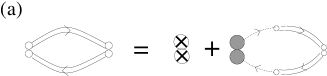
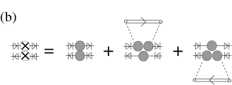
Figure 20: (a) The particle-hole propagator expressed through $\uuline{Q}{}$ and $\uuline{\Lambda}{}\>\uuline{\tilde{G}\tilde{G}}{}$. (b) The quantity $\uuline{\Lambda}{}\>\uuline{\tilde{G}\tilde{G}}{}$ where the external lines are made explicitly for clarity.

Inserting the Dyson equation (36) and using $\sum_{\underline{k}}\underaccent{\approx}{t}_{\underline{k}}=0$, the particle-hole propagator can be separated into a momentum-dependent and momentum-independent part

$$\uuline{P}{}({\underline{q}},i\nu_{n}\,|\,i\omega_{1})$$ (51)

$$=\uuline{\Lambda}{}(i\nu_{n}\,|\,i\omega_{1})\,\uuline{\tilde{G}\tilde{G}}{}(i\nu_{n}\,|\,i\omega_{1})+\uuline{Q}{}({\underline{q}},i\nu_{n}\,|\,i\omega_{1}),$$

with the momentum dependency fully accounted for by the function

$$\uuline{Q}{}({\underline{q}},i\nu_{n}\,|\,i\omega_{1})$$ (52)

$$=\frac{1}{N}\sum_{\underline{k}}\uuline{GG}{}(q,i\nu_{n}|{\underline{k}}|i\omega_{1})\>\>\uuline{tt}{}({\underline{q}}\,|\,{\underline{k}})\>\uuline{\tilde{G}\tilde{G}}{}(i\nu_{n}\,|\,i\omega_{1})$$

and

$$\uuline{\Lambda}{}(i\nu_{n}\,|\,i\omega_{1}) =\uuline{1}{}+\underaccent{\approx}{1}\otimes\big{[}\underaccent{\approx}{\tilde{G}}(i\omega_{1}\!+\!i\nu_{n})\>\underaccent{\approx}{T}(i\omega_{1}\!+\!i\nu_{n})\big{]}$$

$$+\big{[}\underaccent{\approx}{T}(i\omega_{1})\>\underaccent{\approx}{\tilde{G}}(i\omega_{1})\big{]}\otimes\underaccent{\approx}{1}.$$ (53)

This decomposition is show in Fig. 20. The function $\uuline{\Lambda}{}\,\uuline{\tilde{G}\tilde{G}}{}$ is represented graphically as two circles with crosses and incorporates processes, where only one electron leaves a site and propagates through the lattice, while the other remains at this site.

The negative signs in front of the particle-hole propagators in Eq. (47) stem from the closed Fermion loop, i.e. from the permutations necessary to obtain the ordering of the creation- and annihilation operators. Such signs are viewed as part of the diagrammatic rules and thus do not explicitly occur in the figures.

In the Bethe-Salpeter equation (47) the amputated version of the local vertex is used which is obtained by factorizing the one-particle contributions of the local site,

$$\uuline{\Pi}{}(i\nu_{n}\,|\,i\omega_{1},i\omega_{2})=$$ (54)

$$\uuline{\tilde{G}\tilde{G}}{}(i\nu_{n}\,|\,i\omega_{2})\>\uuline{\Pi}{}^{\mathrm{amp}}(i\nu_{n}\,|\,i\omega_{1},i\omega_{2})\>\uuline{\tilde{G}\tilde{G}}{}(i\nu_{n}\,|\,i\omega_{1}).$$

This is done in order to avoid over-counting of contributions from the start- and endpoint of the propagation. Graphically, amputation is indicated by the vertical bars around the arrows.

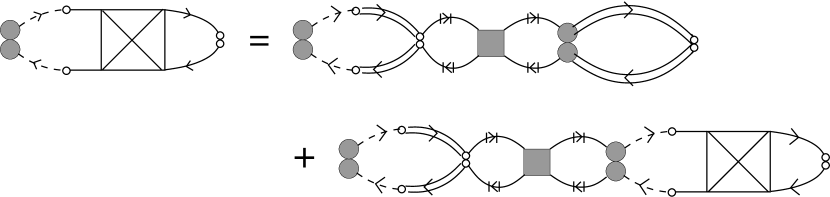
Figure 21: Equation for the two-particle cumulant transfer propagator $\uuline{S}{}^{c}$.

In Eq. (47) an additional quantity $\uuline{S}{}^{c}$ had to be introduced in order to avoid two local irreducible vertices $\Pi$ occuring at the same site right after each other. This two-particle cumulant transfer-propagator describes correlated particle-hole propagations starting with two elementary transfers. A separate Bethe-Salpeter equation can be formulated

$$\uuline{S}{}^{c}({\underline{q}},i\nu_{n}\,|\,i\omega_{1},i\omega_{2})=$$ (55)

$$\uuline{P}{}({\underline{q}},i\nu_{n}\,|\,i\omega_{2})\>\uuline{\Pi}{}^{\mathrm{amp}}(i\nu_{n}\,|\,i\omega_{1},i\omega_{2})\>\uuline{Q}{}({\underline{q}},i\nu_{n}\,|\,i\omega_{1})-$$

$$\sum_{i\omega_{3}}\uuline{S}{}^{c}({\underline{q}},i\nu_{n}\,|\,i\omega_{3},i\omega_{2})\>\uuline{\Pi}{}^{\mathrm{amp}}(i\nu_{n}\,|\,i\omega_{1},i\omega_{3})\>\uuline{Q}{}({\underline{q}},i\nu_{n}\,|\,i\omega_{1}),$$

which is shown graphically in Fig. 21. The crossed box signals, that only terms with at least one local irreducible interaction vertex $\Pi$ involving all four external lines contributes.

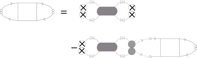
Figure 22: Alternative Bethe-Salpeter equations for the lattice susceptibility expressed with the effective local two-particle cumulant Green functions.

Within DMFT, the local irreducible two-particle vertex $\Pi$ can in principle be determined from the effective impurity model. But it is more instructive to to re-arrange the Bethe-Salpeter equation (47) in terms of dressed local two-particle Green functions, analogous to the one-particle Dyson equation (36). The lattice susceptibility can then be expressed as

$$\uuline{\chi}{}({\underline{q}},i\nu_{n}\,|\,i\omega_{1},i\omega_{2})=\sum_{i\omega_{3}}\Big{[}\uuline{\Lambda}{}(i\nu_{n}\,|\,i\omega_{2})\>\delta_{\omega_{2},\omega_{3}}$$ (56)

$$\phantom{=}-\uuline{\tilde{G}\tilde{G}}{}(i\nu_{n}\,|\,i\omega_{2})\>\uuline{S}{}^{\mathrm{amp}}({\underline{q}},i\nu_{n}\,|\,i\omega_{3},i\omega_{2})\Big{]}\times$$

$$\phantom{==============}\times\uuline{\tilde{G}}{}^{2,\Lambda}(i\nu_{n}\,|\,i\omega_{1},i\omega_{3}).$$

where the amputated two-particle transfer propagator $\uuline{S}{}^{\mathrm{amp}}$ is introduced. This equation is depicted in Fig. 22. The (un-amputated) two-particle transfer propagator $\uuline{S}{}$ is closely related to the two-particle cumulant transfer propagator $\uuline{S}{}^{c}$ via

$$\uuline{S}{}({\underline{q}},i\nu_{n}\,|\,i\omega_{1},i\omega_{2}) =-\uuline{Q}{}({\underline{q}},i\nu_{n}\,|\,i\omega_{1})\delta_{i\omega_{1},i\omega_{2}}$$ (57)

$$+\uuline{S}{}^{c}({\underline{q}},i\nu_{n}\,|\,i\omega_{1},i\omega_{2}).$$

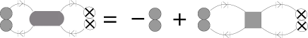
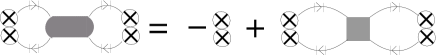
Figure 23: The effective local two-particle cumulant Green functions $\uuline{\tilde{G}}{}^{2}$, $\uuline{\tilde{G}}{}^{2,\Lambda}$, $\uuline{\Lambda}{}\uuline{\tilde{G}}{}^{2,\Lambda}\uuline{\Lambda}{}^{-1}$ (see footnote Note, 2), and $\uuline{\Lambda}{}\uuline{\tilde{G}}{}^{2,\Lambda}$ (from top to bottom).

The dressed local two-particle Green function entering Eq. (56) is

$$\uuline{\tilde{G}}{}^{2,\Lambda}(i\nu_{n}\,|\,i\omega_{1},i\omega_{2}) =-\uuline{\tilde{G}\tilde{G}}{}(i\nu_{n}\,|\,i\omega_{1})\>\delta_{i\omega_{1},i\omega_{2}}$$ (58)

$$+\uuline{\Pi}{}(i\nu_{n}\,|\,i\omega_{1},i\omega_{2})\>\uuline{\Lambda}{}(i\nu_{n}\,|\,i\omega_{1}),$$

which is shown graphically in Fig. 23. It is essentially determined by the local irreducible vertex but additional pseudo-local corrections due to one-particle propagations do occur. The minus sign associated with the first term reflects the fact that this term originates from the particle-hole propagator. Since the closed fermion loop is no longer visible in the diagrammatic representation it is included explicitly in the graphical representation.

The factor of $\uuline{\Lambda}{}$ appearing at the cumulant vertex in Eq. (58) is not valid by the rules of the original cumulant perturbation theory, as two local contributions are multiplied at the very same lattice site. The reason it appears here lies in the internal momentum sums already performed in the lattice susceptibility $\uuline{\chi}{}({\underline{q}},i\nu_{n}\,|\,i\omega_{1},i\omega_{2})$ (see Eq. (45)) together with the approximation of a momentum independent vertex. Separating pseudo-local and nonlocal contributions the momentum-independent part of the particle-hole propagator inevitably leads to the appearance of such terms which are originally not allowed.

Equation (56) is the two-particle analog of the Dyson equation (36) with 1PI diagrams replaced by 2PI diagrams, along with the resulting factors of $\uuline{\Lambda}{}$, and the complication of a second equation needed for the two-particle transfer propagator $\uuline{S}{}$.

For the mapping onto the effective impurity model we construct the local two-particle susceptibility by iterating Eq. (56) once and summing over ${\underline{q}}$ which gives

$$\uuline{\chi}{}^{\mathrm{loc}}(i\nu_{n}\,|\,i\omega_{1},i\omega_{2}) \equiv\frac{1}{N}\sum_{\underline{q}}\uuline{\chi}{}({\underline{q}},i\nu_{n}\,|\,i\omega_{1},i\omega_{2})$$

$$=\uuline{\Lambda}{}(i\nu_{n}\,|\,i\omega_{2})\,\uuline{\tilde{G}}{}^{2,\Lambda}(i\nu_{n}\,|\,i\omega_{1},i\omega_{2})$$ (59)

$$+\sum_{i\omega_{3},i\omega_{4}}\uuline{\Lambda}{}(i\nu_{n}\,|\,i\omega_{2})\uuline{\tilde{G}}{}^{2,\Lambda}(i\nu_{n}\,|\,i\omega_{4},i\omega_{2})\uuline{\Lambda}{}(i\nu_{n}\,|\,i\omega_{4})^{-1}\,\uuline{TT}{}(i\nu_{n}\,|\,i\omega_{3},i\omega_{4})\,\uuline{\tilde{G}}{}^{2,\Lambda}(i\nu_{n}\,|\,i\omega_{1},i\omega_{3}).$$

This equation is represented in Fig. 24. The quantity $\uuline{TT}{}$ is closely related to the ${\underline{q}}$-summed two-particle transfer propagator and represents the two-particle scattering matrix, where both particles leave the local site and propagate through the lattice. Equation (59) is the analog of the one-particle equation (38) and establishes the connection between the effective local two-particle cumulant Green function $\uuline{G}{}^{2,\Lambda}$ (or equivalently the local cumulant vertex $\uuline{\Pi}{}^{c}$) and the local physical Green function.

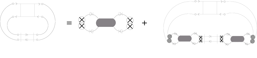
Figure 24: Bethe-Salpeter equation for the local two-particle Green function $\uuline{\chi}{}^{\mathrm{loc}}$.

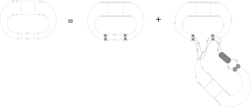
Figure 25: The decomposition of the two-particle scattering matrix $\uuline{TT}{}$ into irreducible propagations $\uuline{\widetilde{TT}}{}$ and repeated visits to the local site.

In complete analogy to the one-particle case (see Eq. (42)) the two-particle scattering matrix $\uuline{TT}{}$ is build up from an irreducible scattering matrix $\uuline{\widetilde{TT}}{}$. The latter describes the simultaneous propagation of two particles starting and ending at the same site without any intermediate returns to this specific site. This decomposition is shown graphical in Fig. 25 which reads analytically

$$\uuline{TT}{}(i\nu_{n}\,|\,i\omega_{1},i\omega_{2})=\sum_{i\omega_{3}}\Big{[}\uuline{\Lambda}{}(i\nu_{n}\,|\,i\omega_{2})\,\delta_{\omega_{3},\omega_{2}}$$ (60)

$$+\sum_{i\omega_{4}}\uuline{TT}{}(i\nu_{n}\,|\,i\omega_{4},i\omega_{2})\,\uuline{\tilde{G}}{}^{2,\Lambda}(i\nu_{n}\,|\,i\omega_{3},i\omega_{4})\Big{]}\times$$

$$\phantom{=====}\times\uuline{\widetilde{TT}}{}(i\nu_{n}\,|\,i\omega_{1},i\omega_{3})\,\uuline{\Lambda}{}(i\nu_{n}\,|\,i\omega_{1}).$$

The structural difference of this equation to the one-particle case Eq. (42) lies in the appearance of the factors $\uuline{\Lambda}{}$ which account for the single-electron recurrence.

At this point the identity

$$\sum_{i\omega_{3}}\uuline{TT}{}(i\nu_{n}\,|\,i\omega_{3},i\omega_{2})\,\uuline{\tilde{G}}{}^{2,\Lambda}(i\nu_{n}\,|\,i\omega_{1},i\omega_{3})$$ (61)

$$=\sum_{i\omega_{3}}\uuline{\Lambda}{}(i\nu_{n}\,|\,i\omega_{2})\,\uuline{\widetilde{TT}}{}(i\nu_{n}\,|\,i\omega_{3},i\omega_{2})\,\uuline{\chi}{}^{\mathrm{loc}}(i\nu_{n}\,|\,i\omega_{1},i\omega_{3})$$

and the equivalent form with the order of the matrix products reversed (as well as the order of the factors $\uuline{\Lambda}{}$) can be proven by comparing Eqs. (59) and (60). These reflect the two possible ways to decompose the local Green function and the effective local cumulant in terms of reducible and irreducible loops.

Utilizing the above identities in Eq. (59), the scattering matrix can be eliminated in favor of the irreducible scattering matrix and the local susceptibility,

$$\uuline{\chi}{}^{\mathrm{loc}}(i\nu_{n}\,|\,i\omega_{1},i\omega_{2})=$$ (62)

$$\uuline{\Lambda}{}(i\nu_{n}\,|\,i\omega_{2})\,\uuline{\tilde{G}}{}^{2,\Lambda}(i\nu_{n}\,|\,i\omega_{1},i\omega_{2})$$

$$+\sum_{i\omega_{3},i\omega_{4}}\uuline{\chi}{}^{\mathrm{loc}}(i\nu_{n}\,|\,i\omega_{3},i\omega_{2})\,\uuline{\widetilde{TT}}{}(i\nu_{n}\,|\,i\omega_{4},i\omega_{3})\times$$

$$\times\uuline{\Lambda}{}(i\nu_{n}\,|\,i\omega_{4})\,\uuline{\tilde{G}}{}^{2,\Lambda}(i\nu_{n}\,|\,i\omega_{1},i\omega_{4}).$$

All equations derived so far incorporate inner frequency sums and thus have the character of integral equations. The local susceptibility $\chi^{\mathrm{loc}}$ is determined from solution of the impurity model and then used as an input functions for Eq. (62). From this, ${\tilde{G}}^{2,\Lambda}$ is determined which then has to be used to solve the lattice equations, Eqs. (56) and (55). Thus, closed explicit expressions for the momentum dependent susceptibilities cannot be obtained, in contrast to the single-particle case.

In order to complete the mapping onto the effective impurity model we need to specify the processes to be incorporated into the effective medium. Therefore, it is beneficial to analyze the structure of this set of equations by switching to the Matsubara-matrix notation. Equation (62) can be solved in Matsubara-matrix space to give

$$\uuline{\hat{\chi}}{}^{\mathrm{loc}}_{i\nu} =\Big{[}\left(\hat{\uuline{\Lambda}{}\uuline{\tilde{G}}{}}^{2,\Lambda}_{i\nu}\right)^{-1}-\uuline{\hat{\widetilde{TT}}}{}_{i\nu}\Big{]}^{-1}.$$ (63)

This clearly demonstrates the resemblance to the one-particle equation (43). The dressed local two-particle Green function is given by $\uuline{\Lambda}{}\uuline{\tilde{G}}{}^{2,\Lambda}$, where the one-particle recurrence problem leads to the unexpected factor of $\uuline{\Lambda}{}$, and $\uuline{\widetilde{TT}}{}$ is the irreducible effective two-particle medium. The effective local two-particle vertex can now be expressed in terms of the local susceptibility function and used to obtain an explicit form for the lattice susceptibility in Matsubara-matrix space

$$\uuline{\hat{\chi}}{}_{{\underline{q}},i\nu_{n}} =\left[-\uuline{\hat{P}}{}_{{\underline{q}},i\nu_{n}}^{-1}+{\uuline{\hat{\chi}}{}^{\mathrm{loc}}_{i\nu_{n}}}^{-1}+\left(\uuline{\Lambda}{}\uuline{\tilde{G}\tilde{G}}{}_{i\nu_{n}}\right)^{-1}+\uuline{\hat{\widetilde{TT}}}{}_{i\nu_{n}}\right]^{-1}.$$ (64)

As the effective impurity is embedded into an noninteracting medium within the DMFT, the irreducible two-particle medium $\uuline{\widetilde{TT}}{}$ can be specified in terms of the effective medium for the one-particle Green function,

$$\uuline{\widetilde{TT}}{}(i\nu_{n}\,|\,i\omega_{1},i\omega_{2})=$$ (65)

$$-\left(\underaccent{\approx}{\Gamma}(i\omega_{1})\otimes\underaccent{\approx}{\Gamma}(i\omega_{1}+i\nu_{n})\right)\,\uuline{\Lambda}{}(i\nu_{n}\,|\,i\omega_{1})^{-1}\delta_{\omega_{1},\omega_{2}}.$$

The negative sign reflects the fact that the effective medium is derived from the ${\underline{q}}$-summed particle-hole propagator, where a minus sign has to be included due to the closed fermion-loop. The factor of $\underaccent{\approx}{\Lambda}^{-1}$ removes those processes where only one electron intermediately re-visits the site, which are present in the product of the two one-particle media $\Gamma$. This is necessary as $\uuline{\widetilde{TT}}{}$ characterizes the amplitude where both electrons must simultaneously leave the local site.

Notice that in this approximation the scattering matrix $\uuline{TT}{}$ is not just the product of the uncorrelated one-particle scattering matrices, i.e.

$$\uuline{TT}{}(i\nu_{n}\,|\,i\omega_{1},i\omega_{2}) \neq-\underaccent{\approx}{T}(i\omega_{1})\otimes\underaccent{\approx}{T}(i\omega_{1}+i\nu_{n})\delta_{\omega_{1},\omega_{2}},$$ (66)

as it could be suspected naïvely. The reason is that two-particle correlations are discarded only in the medium, but locally all interaction vertices are retained. The Matsubara-matrix space representation reveals the structure of $\uuline{TT}{}$

$$\uuline{TT}{}=-\left(\underaccent{\approx}{T}\otimes\underaccent{\approx}{T}\right)\,\left[1+\uuline{\Pi}{}\left(\underaccent{\approx}{T}\otimes\underaccent{\approx}{T}\right)\right]^{-1}.$$ (67)

This very instructive form confirms the insight, that the uncorrelated one-particle loops get renormalized by interaction vertices whenever the particles visit the local lattice site.

The explicit form (65) can be used to express the irreducible scattering matrix as

$$\uuline{\widetilde{TT}}{}(i\nu_{n}|i\omega_{1},i\omega_{2}) =\Big{[}{\uuline{P}{}^{\mathrm{loc}}(i\nu_{n}|i\omega_{1})}^{-1}$$ (68)

$$-\left(\uuline{\Lambda}{}(i\nu_{n}\,|\,i\omega_{1})\,\uuline{\tilde{G}\tilde{G}}{}(i\nu_{n}\,|\,i\omega_{1})\right)^{-1}\Big{]}\delta_{\omega_{1},\omega_{2}},$$

where the local particle-hole propagator is

$$\uuline{P}{}^{\mathrm{loc}}(i\nu_{n}|i\omega_{1}) =\frac{1}{N}\sum_{{\underline{q}}}\uuline{P}{}({\underline{q}},i\nu_{n}\,|\,i\omega_{1})$$ (69)

$$=\underaccent{\approx}{G}^{\mathrm{loc}}(i\omega_{1})\otimes\underaccent{\approx}{G}^{\mathrm{loc}}(i\omega_{1}+i\nu_{n}).$$

Inserting this into the Eq. (64) yields the final form for the lattice susceptibility as stated in Eq. (15).

As stated in the main text, the Matsubara-matrix formalism is not used in this work. Instead, the analytic continuation of all Matsubara frequencies to the real axis is the principal goal of the above treatment. This seems possible, as the local susceptibility function $\uuline{\chi}{}^{\mathrm{loc}}(i\nu_{n}|i\omega_{1},i\omega_{2})$ along with its analytical continuations to the real axis $\uuline{\chi}{}^{\mathrm{loc}}(\nu_{n}\pm i0^{+}|\omega_{1}\pm i0^{+},\omega_{2}\pm i0^{+})$ could be obtained from the effective impurity model. Equation (62), along with the irreducible scattering matrix (65), can be continued to the real axis and the integral equation can be solved for the local two-particle Green functions $\uuline{G}{}^{2,\Lambda}(\nu_{n}\pm i0^{+}|\omega_{1}\pm i0^{+},\omega_{2}\pm i0^{+})$. These are then used to determine the lattice susceptibility function at the real axis via Eqs. (56) and (55).

In practice, this procedure is rather involved and more importantly the extraction of the analytically continued two-particle Green function $\uuline{\chi}{}^{\mathrm{loc}}(\nu_{n}\pm i0^{+}|\omega_{1}\pm i0^{+},\omega_{2}\pm i0^{+})$ from the impurity model is far from trivial and strongly depends on the impurity solver. It is straight forward (but very cumbersome) within semi-analytical approaches like ENCA, where one has a direct handle on the analytic structure of the this function. But, for example, in QMC or NRG it is conceptual not clear how extract two-particle quantities at the real axis.

In order to circumvent this involved procedure, we revert to an additional approximation. The summations over inner Matsubara frequencies are decoupled in a manner similar to the random phase approximation (RPA), i.e.

$$\sum_{i\omega_{3}}\uuline{A}{}(i\nu_{n}\,|\,i\omega_{3},i\omega_{2})\uuline{B}{}(i\nu_{n}\,|\,i\omega_{1},i\omega_{3})$$ (70)

$$\phantom{M}\Rightarrow\uuline{A}{}(i\nu_{n}\,|\,i\omega_{1},i\omega_{2})\sum_{i\omega_{3}}\uuline{B}{}(i\nu_{n}\,|\,i\omega_{1},i\omega_{3}).$$

With this, the inner frequency summations over $i\omega_{1}$ and $i\omega_{2}$ can be performed and the equations can be solved explicity to yield the final form for the susceptibility displayed in Eq. (16).

The local and lattice particle-hole propagators entering this equation can be calculated at the real axis using standard techniques for the evaluation of Matsubara sums,

$$\uuline{P}{}^{\mathrm{loc}}(\nu)=\int\limits_{-\infty}^{\infty}\!d\omega\>f(\omega)\Big{[}\underaccent{\approx}{\rho}(\omega)\otimes\underaccent{\approx}{G}(\omega\!+\!\nu\!+\!i\delta)$$ (71)

$$\phantom{\int_{-\infty}^{\infty}\!d\omega\>f(\omega)\Big{[}}+\underaccent{\approx}{G}(\omega\!-\!\nu\!-\!i\delta)\otimes\underaccent{\approx}{\rho}(\omega)\Big{]}$$

$$\uuline{P}{}({\underline{q}},\nu)=$$ (72)

$$\int\limits_{-\infty}^{\infty}\!d\omega\int\limits_{\mathrm{BZ}}\!\frac{d^{D}{\underline{k}}}{(2\pi)^{D}}f(\omega)\Big{[}\underaccent{\approx}{\rho}({\underline{k}},\omega)\otimes\underaccent{\approx}{G}({\underline{k}}\!+\!{\underline{q}},\omega\!+\!\nu\!+\!i\delta)$$

$$\phantom{\int_{-\infty}^{\infty}\!d\omega MM}+\underaccent{\approx}{G}({\underline{k}},\omega\!-\!\nu\!-\!i\delta)\otimes\underaccent{\approx}{\rho}({\underline{k}}\!+\!{\underline{q}},\omega)\Big{]},$$

with the spectral functions

$$\underaccent{\approx}{\rho}({\underline{k}},\omega) =-\frac{1}{2\pi i}\left(\underaccent{\approx}{G}({\underline{k}},\omega\!+\!i\delta)-\underaccent{\approx}{G}({\underline{k}},\omega\!-\!i\delta)\right)$$ (73)

$$\underaccent{\approx}{\rho}(\omega) =\int\limits_{\mathrm{BZ}}\!\frac{d^{D}{\underline{k}}}{(2\pi)^{D}}\underaccent{\approx}{\rho}({\underline{k}},\omega).$$ (74)

All momentum integrals are over the whole Brillouin-Zone (BZ) in $D$ space dimensions.

References

- Fazekas (1999) P. Fazekas, Lecture Notes on Electron Correlation and Magnetism, Series in Modern Condensed Matter Physics, Vol. 5 (World Scientific, Singapore, 1999).
- Yosida (1996) K. Yosida, Theory of Magnetism, Springer Series in Solid-State Sciences, Vol. 122 (Springer, 1996).
- Plakida (2010) N. Plakida, High-Temperature Cuprate Superconductors, edited by M. Cardona, P. Fulde, K. von Klitzing, R. Merlin, H.-J. Queisser, and H. S. o, Springer Series in solid-state sciences, Vol. 166 (Springer, 2010).
- Grewe and Steglich (1991) N. Grewe and F. Steglich, “Handbook on the physics and chemistry of rare earths,” (North-Holland, 1991) p. 343.
- Coleman (2007) P. Coleman, “Handbook of magnetism and advanced magnetic materials,” (John Wiley and Sons, Ltd., 2007) (preprint at http://archiv.org/abs/cond-mat/0612006).
- Lacroix et al. (2011) C. Lacroix, P. Mendels, and F. Mila, eds., Introduction to Frustrated MagnetismIntroduction to Frustrated Magnetism, Springer Series in Solid-State Sciences, Vol. 164 (Springer, 2011).
- Hopkinson and Coleman (2002) J. Hopkinson and P. Coleman, Phys. Rev. Lett. 89, 267201 (2002).
- Jönsson et al. (2007) P. E. Jönsson, K. Takenaka, S. Niitaka, T. Sasagawa, S. Sugai, and H. Takagi, Phys. Rev. Lett. 99, 167402 (2007).
- Arita et al. (2007) R. Arita, K. Held, A. V. Lukoyanov, and V. I. Anisimov, Phys. Rev. Lett. 98, 166402 (2007).
- Kagawa et al. (2004) F. Kagawa, T. Itou, K. Miyagawa, and K. Kanoda, Phys. Rev. B 69, 064511 (2004).
- Ohashi et al. (2008a) T. Ohashi, T. Momoi, H. Tsunetsugu, and N. Kawakami, Phys. Rev. Lett. 100, 076402 (2008a).
- Ohashi et al. (2008b) T. Ohashi, T. Momoi, H. Tsunetsugu, , and N. Kawakami, Prog. Theor. Phys. Supplemen 176, 97 (2008b).
- Vojta (2009) M. Vojta, Nat. Phys. 5, 623 (2009).
- He et al. (2011) R.-H. He, M. Fujita, M. Enoki, M. Hashimoto, S. Iikubo, S.-K. Mo, H. Yao, T. Adachi, Y. Koike, Z. Hussain, Z.-X. Shen, and K. Yamada, Phys. Rev. Lett. 107, 127002 (2011).
- Tacon et al. (2011) M. L. Tacon, G. Ghiringhelli, J. Chaloupka, M. M. Sala, V. Hinkov, M. W. Haverkort, M. Minola, M. Bakr, K. J. Zhou, S. Blanco-Canosa, C. Monney, Y. T. Song, G. L. Sun, C. T. Lin, G. M. D. Luca, M. Salluzzo, G. Khaliullin, T. Schmitt, L. Braicovich, and B. Keimer, Nat. Phys. 7, 725 (2011).
- Vollhardt et al. (1999) D. Vollhardt, N. Blümer, K. Held, M. Kollar, J. Schlipf, M. Ulmke, and J. Wahle, Adv. Solid State Phys. 38, 383 (1999).
- Pruschke et al. (1995) T. Pruschke, M. Jarrell, and J. Freericks, Adv. Phys. 44, 187 (1995).
- Georges et al. (1996) A. Georges, G. Kotliar, W. Krauth, and M. J. Rozenberg, Rev. Mod. Phys. 68, 13 (1996).
- A.Georges (2004) A.Georges, in Lectures on the physics of highly correlated electron systems VIII, AIP Conf. Proc., Vol. 715, edited by A.Avella and F.Mancini (2004) pp. 3–74.
- Jarrell (1992) M. Jarrell, Phys. Rev. Lett. 69, 168 (1992).
- Zlatic and Horvatic (1990) V. Zlatic and B. Horvatic, Solid State Commun. 75, 263 (1990).
- Jarrell (1995) M. Jarrell, Phys. Rev. B 51, 7429 (1995).
- Toschi et al. (2007) A. Toschi, A. A. Katanin, and K. Held, Phys. Rev. B 75, 045118 (2007).
- Kuneš (2011) J. Kuneš, Phys. Rev. B 83, 085102 (2011).
- Lieb and Wu (1968) E. H. Lieb and F. Wu, Phys. Rev. Lett. 20, 1445 (1968).
- Lieb and Wu (2003) E. H. Lieb and F. Y. Wu, Physica A 321, 1 (2003).
- Essler et al. (2005) F. Essler, H. Frahm, F. Göhmann, A. Klümper, and V. Korepin, The One-Dimensional Hubbard Model (2005).
- Metzner and Vollhardt (1989) W. Metzner and D. Vollhardt, Phys. Rev. Lett. 62, 324 (1989).
- Müller-Hartmann (1989a) E. Müller-Hartmann, Z. Phys. B 74, 507 (1989a).
- Caffarel and Krauth (1994) M. Caffarel and W. Krauth, Phys. Rev. Lett. 72, 1545 (1994).
- Si et al. (1994) Q. Si, M. J. Rozenberg, G. Kotliar, and A. E. Ruckenstein, Phys. Rev. Lett. 72, 2761 (1994).
- Hirsch and Fye (1986) J. E. Hirsch and R. M. Fye, Phys. Rev. Lett. 56, 2521 (1986).
- Gull et al. (2011) E. Gull, A. J. Millis, A. I. Lichtenstein, A. N. Rubtsov, M. Troyer, and P. Werner, Rev. Mod. Phys. 83, 349 (2011).
- Wilson (1975) K. G. Wilson, Rev. Mod. Phys. 47, 773 (1975).
- Bulla et al. (2008) R. Bulla, T. Costi, and T. Pruschke, Rev. Mod. Phys. 80, 395 (2008).
- Pruschke and Grewe (1989) T. Pruschke and N. Grewe, Z. Phys. B 74, 439 (1989).
- Schmitt et al. (2009) S. Schmitt, T. Jabben, and N. Grewe, Phys. Rev. B 80, 235130 (2009).
- Grewe et al. (2008) N. Grewe, S. Schmitt, T. Jabben, and F. B. Anders, J. Phys.: Condens. Matter 20, 365217 (2008).
- Holm and Schönhammer (1989) J. Holm and K. Schönhammer, Solid State Commun. 69, 969 (1989).
- Keiter and Qin (1990) H. Keiter and Q. Qin, Physica B 163, 594 (1990).
- Jarrell and Gubernatis (1996) M. Jarrell and J. E. Gubernatis, Phys. Rep. 269, 133 (1996).
- Raas and Uhrig (2005) C. Raas and G. S. Uhrig, Eur. Phys. J. B 45, 293 (2005).
- Raas and Uhrig (2009) C. Raas and G. S. Uhrig, Phys. Rev. B 79, 115136 (2009).
- Schmitt and Grewe (2005) S. Schmitt and N. Grewe, Physica B 359-361, 777 (2005).
- Schmitt (2009) S. Schmitt, Excitations, Two-Particle Correlations and Ordering Phenomena in Strongly Correlated Electron Systems from a Local Point of View, Ph.D. thesis, TU Darmstadt (2009), available at http://tuprints.ulb.tu-darmstadt.de/1264/.
- Note (1) As two-particle quantities –in contrast to single-particle Green functions– do not depend on the sign of the infinitesimal imaginary part , we omit it here.
- Doniach and Sondheimer (1974) S. Doniach and E. H. Sondheimer, Green’s Functions for Solid State Physicists (W. A. Benjamin, Inc, 1974).
- Schäfer and Schuck (1999) S. Schäfer and P. Schuck, Phys. Rev. B 59, 1712 (1999).
- Bickers et al. (1989) N. E. Bickers, D. J. Scalapino, and S. R. White, Phys. Rev. Lett. 62, 961 (1989).
- Bickers and White (1991) N. E. Bickers and S. R. White, Phys. Rev. B 43, 8044 (1991).
- Vilk et al. (1994) Y. M. Vilk, L. Chen, and A.-M. S. Tremblay, Phys. Rev. B 49, 13267 (1994).
- Khaliullin and Horsch (1996) G. Khaliullin and P. Horsch, Phys. Rev. B 54, R9600 (1996).
- Saikawa and Ferraz (1998) T. Saikawa and A. Ferraz, Eur. Phys. J. B 3, 17 (1998).
- Eremin et al. (2001) M. Eremin, I. Eremin, and S. Varlamov, Phys. Rev. B 64, 214512 (2001).
- Uldry and Elliott (2005) A. Uldry and R. J. Elliott, J. Phys.: Condens. Matter 17, 2903 (2005).
- Moskalenko and Plakida (1997) V. A. Moskalenko and N. M. Plakida, Theor. Math. Phys. 113, 1309 (1997).
- Sherman and Schreiber (2007) A. Sherman and M. Schreiber, Phys. Rev. B 76, 245112 (2007).
- Sherman and Schreiber (2008) A. Sherman and M. Schreiber, Phys. Rev. B 77, 155117 (2008).
- Hanisch et al. (1997) T. Hanisch, G. S. Uhrig, and E. Müller-Hartmann, Phys. Rev. B 56, 13960 (1997).
- Hanisch et al. (1995) T. Hanisch, B. Kleine, A. Ritzl, and E. Müller-Hartmann, Ann. Physik 507, 303 (1995).
- Hanisch (1996) T. Hanisch, Gitterabhängigkeit des Ferromagnetismus im Hubbad-Modell, Ph.D. thesis, Universität zu Köln, Köln (1996).
- Hahn (2005) T. Hahn, Comput. Phys. Commun. 168, 78 (2005), see also http://www.feynarts.de/cuba/.
- Penn (1966) D. R. Penn, Phys. Rev. 142, 350 (1966).
- van Dongen (1991) P. G. J. van Dongen, Phys. Rev. Lett. 67, 757 (1991).
- Staudt et al. (2000) R. Staudt, M. Dzierzawa, and A. Muramatsu, Eur. Phys. J. B 17, 411 (2000).
- Hirsch (1987) J. E. Hirsch, Phys. Rev. B 35, 1851 (1987).
- Scalettar et al. (1989) R. T. Scalettar, D. J. Scalapino, R. L. Sugar, and D. Toussaint, Phys. Rev. B 39, 4711 (1989).
- Ulmke et al. (1996) M. Ulmke, R. T. Scalettar, A. Nazarenko, and E. Dagotto, Phys. Rev. B 54, 16523 (1996).
- Daré and Albinet (2000) A.-M. Daré and G. Albinet, Phys. Rev. B 61, 4567 (2000).
- Vilk and Tremblay (1997) Y. Vilk and A. Tremblay, J. Phys. I 7, 1309 (1997).
- Daré et al. (1996) A.-M. Daré, Y. M. Vilk, and A. M. S. Tremblay, Phys. Rev. B 53, 14236 (1996).
- Arita et al. (2000) R. Arita, S. Onoda, K. Kuroki, and H. Aoki, J. Phys. Soc. Jpn. 69, 785 (2000).
- Jarrell and Pruschke (1993) M. Jarrell and T. Pruschke, Z. Phys. B 90, 187 (1993).
- Ulmke et al. (1995) M. Ulmke, V. Janiš, and D. Vollhardt, Phys. Rev. B 51, 10411 (1995).
- Zitzler et al. (2004) R. Zitzler, N.-H. Tong, T. Pruschke, and R. Bulla, Phys. Rev. Lett. 93, 016406 (2004).
- Freericks and Jarrell (1995) J. K. Freericks and M. Jarrell, Phys. Rev. Lett. 74, 186 (1995).
- Tahvildar-Zadeh et al. (1997) A. N. Tahvildar-Zadeh, J. K. Freericks, and M. Jarrell, Phys. Rev. B 55, 942 (1997).
- Peters and Pruschke (2009a) R. Peters and T. Pruschke, Phys. Rev. B 79, 045108 (2009a).
- Aryanpour et al. (2006) K. Aryanpour, W. E. Pickett, and R. T. Scalettar, Phys. Rev. B 74, 085117 (2006).
- De Leo et al. (2011) L. De Leo, J.-S. Bernier, C. Kollath, A. Georges, and V. W. Scarola, Phys. Rev. A 83, 023606 (2011).
- Kent et al. (2005) P. R. C. Kent, M. Jarrell, T. A. Maier, and T. Pruschke, Phys. Rev. B 72, 060411 (2005).
- Rohringer et al. (2011) G. Rohringer, A. Toschi, A. Katanin, and K. Held, arxiv:1104.1919 (2011).
- Fuchs et al. (2011a) S. Fuchs, E. Gull, M. Troyer, M. Jarrell, and T. Pruschke, Phys. Rev. B 83, 235113 (2011a).
- Fuchs et al. (2011b) S. Fuchs, E. Gull, L. Pollet, E. Burovski, E. Kozik, T. Pruschke, and M. Troyer, Phys. Rev. Lett. 106, 030401 (2011b).
- Grewe (1983) N. Grewe, Z. Phys. B 53, 271 (1983).
- Kuramoto and Müller-Hartmann (1985) Y. Kuramoto and E. Müller-Hartmann, J. Magn. Magn. Mater. 52, 122 (1985).
- Kuramoto and Kojima (1984) Y. Kuramoto and H. Kojima, Z. Phys. B 57, 95 (1984).
- Müller-Hartmann (1984) E. Müller-Hartmann, Z. Phys. B 57, 281 (1984).
- Ulmke (1998) M. Ulmke, Eur. Phys. J. B 1, 301 (1998).
- Byczuk and Vollhardt (2002) K. Byczuk and D. Vollhardt, Phys. Rev. B 65, 134433 (2002).
- Rushbrooke et al. (1974) G. Rushbrooke, G. Baker, and P. Wood, in Phase Transitions and Critical Phenomena, Vol. 3, edited by C. Domb and M. Green (Academic Press, London, New York, 1974) p. 245.
- Grete et al. (2011) P. Grete, S. Schmitt, C. Raas, F. B. Anders, and G. S. Uhrig, Phys. Rev. B 84, 205104 (2011).
- Peters et al. (2006) R. Peters, T. Pruschke, and F. B. Anders, Phys. Rev. B 74, 245114 (2006).
- Igoshev et al. (2010) P. A. Igoshev, M. A. Timirgazin, A. A. Katanin, A. K. Arzhnikov, and V. Y. Irkhin, Phys. Rev. B 81, 094407 (2010).
- Zitzler et al. (2002) R. Zitzler, T. Pruschke, and R. Bulla, Eur. Phys. J. B 27, 473 (2002).
- Nagaoka (1965) Y. Nagaoka, Solid State Commun. 3, 409 (1965).
- Obermeier et al. (1997) T. Obermeier, T. Pruschke, and J. Keller, Phys. Rev. B 56, R8479 (1997).
- Fazekas et al. (1990) P. Fazekas, B. Menge, and E. Müller-Hartmann, Z. Phys. B 78, 69 (1990).
- Merino et al. (2006) J. Merino, B. J. Powell, and R. H. McKenzie, Phys. Rev. B 73, 235107 (2006).
- Peters and Pruschke (2009b) R. Peters and T. Pruschke, New Journal of Physics 1 11, 083022 (2009b).
- Günther et al. (2011) F. Günther, G. Seibold, and J. Lorenzana, Phys. Status Solidi B 248, 339 (2011).
- Schmitt (2010) S. Schmitt, Phys. Rev. B 82, 155126 (2010).
- Müller-Hartmann (1989b) E. Müller-Hartmann, Z. Phys. B 76, 211 (1989b).
- Georges and Krauth (1993) A. Georges and W. Krauth, Phys. Rev. B 48, 7167 (1993).
- Halvorsen and Czycholl (1994) E. Halvorsen and G. Czycholl, J. Phys.: Condens. Matter 6, 10331 (1994).
- Hong et al. (1996) S.-P. Hong, H. Doh, and S.-H. S. Salk, Czech. J. Phys. 46, 1855 (1996).
- Mancini and Avella (2004) F. Mancini and A. Avella, Adv. Phys. 53, 537 (2004).
- Pietig et al. (1999) R. Pietig, R. Bulla, and S. Blawid, Phys. Rev. Lett. 82, 4046 (1999).
- Shen and Davis (2008) K. Shen and J. Davis, Materials Today 11, 14 (2008).
- Metzner (1991) W. Metzner, Phys. Rev. B 43, 8549 (1991).
- Grewe (1996) N. Grewe, “Eine lokale theorie des festkörpers,” (1996), internal Report.
- Craco and Gusmão (1995) L. Craco and M. A. Gusmão, Phys. Rev. B 52, 17135 (1995).
- Note (2) The cumbersome expression just represents , but with the factor of at the other side of the vertex, i.e. (see Fig. 23). This form is used to avoid another abbreviation.