Possibility of superconductivity due to electron-phonon interaction in graphene

Abstract

We discuss the possibility of superconductivity in graphene taking into account both electron-phonon and electron-electron Coulomb interactions. The analysis is carried out assuming that the Fermi energy is far away from the Dirac points, such that the density of the particles (electrons or holes) is high. We derive proper Eliashberg equations that allow us to estimate the critical superconducting temperature. The most favorable is pairing of electrons belonging to different valleys in the spectrum. By using values of electron-phonon coupling estimated in other publications we obtain the critical temperature $T_{c}$ as a function of the electron (hole) density. This temperature can reach the order of $10$ K at the Fermi energy of order $1-2$ eV. We show that the dependence of the intervalley pairing on the impurity concentration should be weak.

I Introduction

Since its experimental discovery in 2004 geim2004 and first observations of unusual properties, novoselov2005 ; kim2005 graphene has gained a lot of experimental and theoretical attraction. In the last decade, thousands of articles devoted to the study of graphene have appeared. Possessing novel electro-mechanical properties, graphene is a promising material for electronic devices. The linear Dirac-type electron spectrum makes graphene very interesting from the theoretical point of view and many interesting effects have been predicted and observed. castro

However, still there are open questions on fundamental electronic properties of graphene, and one of the most interesting ones concerns a possibility of superconductivity. Graphene is a good conductor unless the Fermi energy is too close to the Dirac points and the electron-phonon coupling in graphene is not very weak. Therefore, although the superconductivity in graphene has not been observed, it is not clear why one should discard the possibility of this phenomenon.

Superconductivity can be induced in graphene by superconducting contacts due to the proximity effect, heersche but can it be obtained in a “natural way"? What should one do in order to obtain a considerable value of the superconducting critical temperature $T_{c}$? What type of the superconductivity and what structure of the order parameter could one expect?

In the last years, there have been various attempts to answer these questions. Due to the special type of the spectrum, the main attention has been devoted to investigating the possibility of unusual types of the superconducting pairing. Superconducting pairing mediated by conventional electron-phonon or electron-plasmon coupling was considered in Ref. [uchoa, ] with a conclusion that, in addition to the conventional $s$-wave pairing, an exotic $p+ip$ state is possible. Superconducting properties of Dirac electrons in graphene were considered in Ref. [kopnin, ] within the conventional BCS approach. In these publications, the main emphasis was put on the study of properties of unusual superconducting pairing for a small electron density.

It is clear that one can expect very interesting new properties of the superconductivity in the vicinity of the Dirac points. However, this region is least favorable for the existence of superconductivity due to the very low density of states, and one should tune the Fermi energy away from the Dirac points in order to have a hope to obtain superconductivity.

By doping graphene by various combinations of K and Ca, the authors of Ref. [chesney, ] were able to shift the Fermi energy far away the Dirac points and even to put it in the vicinity of the van Hove singularity (VHS). Another experimental method based on the use of electrolytic gates efetov allowed the authors to tune continuously the electron density up to values $n=4\times 10^{14}\mathrm{cm}^{-2}$, which is apparently not very far away from the VHS. These experimental works have demonstrated that one can achieve a ultrahigh electron density and this makes observation of superconductivity in graphene considerably more realistic. At the same time, transport measurements were not carried out in Ref. [chesney, ] and the superconductivity has not been seen in Ref. [efetov, ] for temperatures $T\gtrsim 1\ \mathrm{K}$.

Although the superconductivity has not been observed yet, theoretical considerations gonzalez ; chubukov ; thomale predict superconductivity at the VHS even for a repulsive electron-electron interaction. In this case, the superconductivity is expected to have an unconventional symmetry of the order parameter. No doubt, an experimental observation of the superconductivity at the VHS would be of a great interest, but one should be able to tune the Fermi energy exactly to the singularity. Disorder may also play a destructive role in formation of such a superconductivity.

Therefore, it would still be important to investigate theoretically the possibility of a superconducting pairing due to the conventional electron-phonon pairing far away from the Dirac point, but, at the same time, not in the vicinity of the VHS. Such a study implies using conventional schemes of computing the superconducting transition temperature. Then, one should check the stability of the pairing against disorder in the system, clarify the dependence of the transition temperature $T_{c}$, etc.

In several publications, models with an electron-phonon interaction have been considered. The authors of Ref. [lozovik, ] discussed the valley structure of the order parameter using an electron-phonon model without the electron-electron Coulomb interaction. They argued that there might be a superconducting instability in highly doped graphene, while the valley structure depends on the parameters of the electron-phonon interaction. Superconductivity in hydrogenized graphene (graphane) has been considered as well. graphane In this system, a model based on electron-phonon interaction was used and a transition temperature of $90\ \mbox{K}$ in p-doped graphane was predicted. At the same time, it is clear that taking into account the Coulomb interaction is very important because it can in principle be even stronger than the electron-phonon interaction. Moreover, considering the latter in the weak coupling limit can also lead to incorrect predictions.

In this paper, we use a generic model including both the electron-phonon and electron-electron Coulomb interactions. Using Eliashberg-type equations,eliashberg ; morel ; mcmillan we derive an expression for the transition temperature determined by the electron and phonon interactions in graphene. By using experimental values and results of numerical calculations for the interactions obtained for the normal state, we estimate the transition temperature $T_{c}$ and conclude that the superconductivity is possible with $T_{c}$ of the order of several Kelvin. Most favorable is a singlet pairing between different valleys. We show that such a pairing is not very sensitive to disorder.

The paper is organized as follows. In Sec. $\mathrm{II}$, we formulate the Hamiltonian of quasiparticles in doped graphene describing the interaction of quasiparticles with phonons and the Coulomb interaction. In Sec. $\mathrm{III}$, we consider the electron pairing by deriving and solving the Eliashberg equations. The effects of impurity scattering are considered in Sec. $\mathrm{IV}$. In Sec. $\mathrm{V}$, estimates are made, and the concluding Sec. $\mathrm{VI}$ is devoted to discussions.

II Model Hamiltonian

In this section, we introduce the Hamiltonian of interacting quasiparticles in a single layer of graphene. For the undoped system, the Fermi surface consists of two nonequivalent points $\mathbf{K}$ and $\mathbf{K}^{\prime}=-\mathbf{K}$, called the Dirac points. castro The quasiparticles around these points have a linear spectrum. This approximation remains valid up to quite high energies. We consider in this work doping levels corresponding to the Fermi energy $\varepsilon_{F}$ of the order of $1\mathrm{eV}$. In other words, we consider the case when the Fermi energy is sufficiently far away from both the Dirac point and the VHS. In this region of parameters the spectrum consists of two well resolved valleys and each valley is a cone. As the Fermi energy is far away from the Dirac points one does not need to account for effects specific for the Dirac equation.

The two valleys are numerated by a variable called isospin. Due to the electron-phonon and electron-electron interactions there are matrix elements of the Hamiltonian mixing these two valleys. As we do not investigate properties of the system near the Dirac point we do not use the Dirac-type representation of the Schrodinger equation.

The Hamiltonian describing the electron-phonon system can be written in a general form

$$\hat{H}=\hat{H}_{0}+\hat{H}_{e,ph}+\hat{H}_{e,e},$$ (1)

where

$$\hat{H}_{0}=\sum_{\mathbf{p,}\sigma}\left(\varepsilon\left(\mathbf{p}\right)-\mu\right)c_{\mathbf{p},\sigma}^{{\dagger}}c_{\mathbf{p},\sigma}$$ (2)

is the operator of the kinetic energy, $\varepsilon\left(\mathbf{p}\right)$ is the spectrum of the non-interacting electrons, $\mu$ is the chemical potential (Fermi energy at low temperatures), $\sigma$ is the spin index, $c_{\mathbf{p},\sigma}\left(c_{\mathbf{p},\sigma}^{{\dagger}}\right)$ is the electron annihilation (creation) operator for the electron with momentum $\mathbf{p}$ and spin $\sigma$, $\hat{H}_{e,ph}$ stands for the electron-phonon interaction, and $\hat{H}_{e,e}$-for the electron-electron one.

II.1 Electron-phonon interaction

The Hamiltonian $\hat{H}_{e,ph}$ describing the interaction between the electrons and phonons can be written in a general form as agd ; grimvall

$$\hat{H}_{e,ph}=\sum_{\mathbf{p,q},j,\sigma}g_{\mathbf{p,q},j}\ \Phi_{\mathbf{q},j}c_{\mathbf{p+q},\sigma}^{{\dagger}}c_{\mathbf{p},\sigma},$$ (3)

where $g_{\mathbf{p},\mathbf{q},j}$ is the electron-phonon coupling function and $\Phi_{\mathbf{q},j}$ is the phonon field operator for the mode $j$. As usual, the most important contributions to the thermodynamics are expected from the vicinity of the Fermi surface that consists in the case involved of two circles.

In order to distinguish explicitly between the valleys we write $c_{\mathbf{K}+\mathbf{p},\sigma}\equiv a_{1,\mathbf{p},\sigma}$ and $c_{\mathbf{K}^{\prime}+\mathbf{p},\sigma}\equiv a_{2,\mathbf{p},\sigma}$ for quasiparticles in the vicinity of the Fermi circles of the two valleys $1$ and $2$, where $a_{\alpha,\mathbf{p,}\sigma},$ $\alpha=1,2$ are fermionic annihilation operators with the momentum $\mathbf{p}$ measured from the Dirac point of the $\alpha$-valley.

Using these notations we write the electron-phonon interaction $\hat{H}_{e,ph}$, Eq. (3), in the form

$$\hat{H}_{e,ph}=\sum_{\alpha,\beta=1}^{2}\sum_{\mathbf{p,q,}j,\sigma}g_{\mathbf{p,q},j}^{\alpha\beta}\ \Phi_{\mathbf{q},j}^{\alpha\beta}a_{\alpha,\mathbf{p+q},\sigma}^{{\dagger}}a_{\beta,\mathbf{p},\sigma}.$$ (4)

In Eq. (4) the coupling constants $g^{\alpha\beta}$ and the phonon field operators are related to those in Eq. (3) as

$$g_{\mathbf{p,q},j}^{11}\ = g_{\mathbf{p-K,q},j},\quad g_{\mathbf{p,q},j}^{22}\ =g_{\mathbf{p-K}^{\prime}\mathbf{,q},j},\quad$$ (5)

$$g_{\mathbf{p,q,}j}^{12} = g_{\mathbf{p-K}^{\prime}\mathbf{,q-Q},j},\quad g_{\mathbf{p,q},j}^{21}=g_{\mathbf{p-K},\mathbf{q+Q},j},$$

$$\Phi_{\mathbf{q},j}^{11} = \Phi_{\mathbf{q},j},\quad\Phi_{\mathbf{q,}j}^{22}=\Phi_{\mathbf{q,}j},\quad$$

$$\Phi_{\mathbf{q},j}^{12} = \Phi_{\mathbf{q-Q},j},\quad\Phi_{\mathbf{q},j}^{21}=\Phi_{\mathbf{q+Q},j},$$

where $\mathbf{Q}=\mathbf{K}^{\prime}-\mathbf{K}$ is the vector connecting the Dirac points. The phonon fields $\Phi$ are real in the coordinate representation and therefore we obtain the following relations

$$\Phi_{-\mathbf{q},j}^{11} = \left(\Phi_{\mathbf{q},j}^{11}\right)^{\ast},\quad\Phi_{-\mathbf{q,}j}^{22}=\left(\Phi_{\mathbf{q,}j}^{22}\right)^{\ast},$$ (6)

$$\Phi_{-\mathbf{q},j}^{12} = \left(\Phi_{\mathbf{q},j}^{21}\right)^{\ast},\quad\Phi_{-\mathbf{q},j}^{21}=\left(\Phi_{\mathbf{q},j}^{12}\right)^{\ast}.$$

In Eq. (4) the sum is taken over such $\mathbf{p}$ and $\mathbf{q}$ that both $\mathbf{p}$ and $\mathbf{p}+\mathbf{q}$ are in the vicinity of the Fermi circle. The terms with $\alpha=\beta$ in the Hamiltonian $\hat{H}_{e,ph}$, Eq. (4) describes the intravalley scattering of electrons by the phonons, while the terms with $\alpha\neq\beta$ stand for the intervalley scattering. Formally, we can speak of an isospin dependence of the electron-phonon interaction.

The bare Hamiltonian $\hat{H}_{0}$, Eq. (2), takes in these notations the form

$$\hat{H}_{0}=\sum_{\alpha=1}^{2}\sum_{\mathbf{p,}\sigma}\xi_{\mathbf{p}}{\alpha}_{\alpha,\mathbf{p,}\sigma}^{{\dagger}}{\alpha}_{\alpha,\mathbf{p,}\sigma},$$ (7)

where the energy $\xi_{\mathbf{p}}$ equals

$$\xi_{\mathbf{p}}=v_{0}\left|\mathbf{p}\right|-\mu,$$ (8)

and $v_{0}\approx 10^{8}~{}\mathrm{cm}\ \mathrm{s}^{-1}$ is the Fermi velocity.

Equations (4)-(7) specify how the presence of the two valleys can be written in terms of the isospin. The coupling constants $g^{\alpha\beta}$ are different for the intravalley and intervalley scattering (equal or unequal $\alpha,\,\beta$, respectively). In graphene, two two-phonon peaks are seen in the Raman spectrum (see, e.g., Refs. ferrari, ; yan, ): the $D^{\ast}$ peak near $2\omega_{A_{1}}=2650\ \mathrm{cm}^{-1}$ corresponding to the scalar $A_{1}$ optical phonons and the $G^{\ast}$ peak near $2\omega_{E_{2}}=3250\ \mathrm{cm}^{-1}$ corresponding to twofold-degenerate pseudovector $E_{2}$ phonon mode. The $E_{2}$ mode is responsible for intravalley scattering, while the scalar $A_{1}$ optical mode leads to the intervalley scattering. basko

II.2 Coulomb interaction

The operator of the electron-electron interaction $\hat{H}_{e,e}$ in Eq. (1) can be written in the standard form

$$\hat{H}_{e,e}=\frac{1}{2}\sum_{\mathbf{p},\mathbf{p}^{\prime},\mathbf{q}}\ V_{\mathbf{q}}\ c_{\mathbf{p+q}}^{{\dagger}}c_{\mathbf{p}^{\prime}-\mathbf{q}}^{{\dagger}}c_{\mathbf{p}^{\prime}}c_{\mathbf{p}},$$ (9)

where $V_{\mathbf{q}}$ is the matrix element of the Coulomb potential in two dimensions. We assume here that corrections to the bare Coulomb potential have already been calculated and use therefore for $V_{\mathbf{q}}$ the static screened Coulomb interaction. Due to a specific form of the wave functions of graphene leading to a suppression of the backscattering, the function $V_{\mathbf{q}}$ differs from the conventional Fourier transform of the Coulomb interaction and can be written in the form

$$V_{\mathbf{q}}=\frac{2\pi e^{2}}{\kappa\left|\mathbf{q}\right|\epsilon(\mathbf{q})}\gamma(\mathbf{q})$$ (10)

where $\kappa$ is the dielectric constant of the substrate, $\epsilon(\mathbf{q})=1+\frac{2\pi e^{2}}{\kappa\left|\mathbf{q}\right|}\Pi\left(\mathbf{q}\right)$ is the static dielectric permeability of the electron gas and

$$\gamma(\mathbf{q})=\frac{1}{2}\left(1+\cos\phi_{\mathbf{q}}\right)$$ (11)

with $\phi_{\mathbf{q}}=\arctan\frac{q_{y}}{q_{x}}$ is the form factor accounting for the absence of backscattering in graphene. The static polarizability $\Pi\left(\mathbf{q}\right)$ is given by Hwang

$$\frac{\Pi(\mathbf{q})}{4\nu}=\qquad\qquad\qquad\qquad\qquad\qquad\qquad$$

$$\left\{\begin{array}[]{ccc}1&\mathrm{for}&q\leq 2p_{F}\\ 1-\frac{1}{2}\sqrt{1-\frac{4p_{F}}{q}}-\frac{q}{4p_{F}}\sin^{-1}\left(\frac{2p_{F}}{q}\right)+\frac{\pi q}{8p_{F}}&\mathrm{for}&q>2p_{F}\end{array}\right.$$ (14)

where

$$\nu\left(\mu\right)=\frac{\mu}{2\pi v_{0}^{2}}$$ (15)

is the density of states per one spin direction and one valley and $p_{F}$ is the Fermi momentum. The factor $4$ in Eq. (14) accounts for the number of the spin and isospin directions.

Again, we can use the isospin formulation to bring the operator $\hat{H}_{e,e}$ to a more convenient form

$$\hat{H}_{e,e}=\frac{1}{2}\sum_{\alpha,\beta}\sum_{\mathbf{p},\mathbf{p}^{\prime},\mathbf{q}}V_{\mathbf{q}}^{\alpha\beta}a_{\alpha,\mathbf{p+q}}^{{\dagger}}a_{\beta,\mathbf{p}^{\prime}-\mathbf{q}}^{{\dagger}}a_{\alpha,\mathbf{p}^{\prime}}a_{\beta,\mathbf{p}},$$ (16)

where

$$V_{\mathbf{q}}^{11} = V_{\mathbf{q}}^{22}=V_{\mathbf{q}},$$ (17)

$$V_{\mathbf{q}}^{12} = V_{\mathbf{q-Q}},\quad V_{\mathbf{q}}^{21}=V_{\mathbf{q+Q}},$$

and the sum in Eq. (16) includes such momenta $\mathbf{p},\mathbf{p}^{\prime}$, and $\mathbf{q}$ that both $\mathbf{p+q}$ and $\mathbf{p}^{\prime}-\mathbf{q}$ are in the vicinity of the Fermi circle.

In the next section we will derive Eliashberg equations for the model described by Eqs. (1), (4), (7), and (16).

III Eliashberg equations

In order to describe the electron pairing mediated by electron-phonon interaction, we derive the Eliashberg equations eliashberg ; mcmillan ; vonsovsky ; carbotte for the system under consideration using conventional methods of quantum field theory. agd We introduce the imaginary time normal and anomalous Green functions that are $4\times 4$ matrices in the valley and spin space

$$\hat{G}_{\mathbf{p}}(\tau)\equiv-\langle T_{\tau}\hat{\psi}_{\mathbf{p}}(0)\hat{\bar{\psi}}_{\mathbf{p}}(\tau)\rangle\quad\hat{F}_{\mathbf{p}}(\tau)\equiv\langle T_{\tau}\hat{\psi}_{\mathbf{-p}}(0)\hat{\psi}_{\mathbf{p}}^{T}(\tau)\rangle,$$ (18)

where the field operators $\psi_{\mathbf{p}}\left(\tau\right)$ are $4$-components vectors having as components the operators $a_{\alpha,\mathbf{p},\sigma}$ in the Heisenberg representation.

In the isospin representation the gap function $\hat{\Delta}_{\mathbf{p},\varepsilon_{n}}$ entering the Gorkov equation is a $4\times 4$ matrix.

Using the normal $\hat{G}_{\mathbf{p},\varepsilon_{n}}$ and anomalous $\hat{F}_{\mathbf{p},\varepsilon_{n}}$ Green functions, we consider the Dyson equations containing both normal and anomalous self-energy parts. Using this matrix representation, we derive the Gorkov equations in the generalized form

$$\left(iZ_{n}\varepsilon_{n}-\xi_{\mathbf{p}}\right)\hat{G}_{\mathbf{p,}\varepsilon_{n}}+Z_{n}\hat{\Delta}_{\mathbf{p},\varepsilon_{n}}F_{\mathbf{p,}\varepsilon_{n}}^{+} = 1$$ (19)

$$\left(iZ_{n}\varepsilon_{n}+\xi_{\mathbf{p}}\right)F_{\mathbf{p,}\varepsilon_{n}}^{+}+Z_{n}\hat{\Delta}_{\mathbf{p},\varepsilon_{n}}^{+}\hat{G}_{\mathbf{p,}\varepsilon_{n}} = 0,$$

where $\varepsilon_{n}=\pi T\left(2n+1\right)$ is the fermionic Matsubara frequency, and the symbol $``+"$ stands for the Hermitian conjugation of the $4\times 4$ matrices.

According to the Eliashberg eliashberg theory developed for an arbitrary value of the coupling in the limit $\omega_{D}\ll\mu$, where $\omega_{D}$ is the Debye frequency, one has to take into account normal contributions of the self-energy to the Green functions, but neglect the renormalization of the vertices. As we assume that both the electron-phonon and electron-electron interactions are not necessarily weak, one should introduce the factor $Z_{n}$ coming from the normal self-energy. This factor renormalizes the coefficient in front of the frequency, but the renormalization of the coefficient for $\xi_{\mathbf{p}}$ is neglected. This non-equivalence originates from the fact that the renormalization of the coefficient in front of the frequency is proportional to $\omega_{D}^{-1},$ while corrections to the coefficient in front of $\xi_{\mathbf{p}}$ are proportional to $\mu^{-1}$. The factor $Z_{n}$ in front of $\hat{\Delta}_{\mathbf{p},\varepsilon_{n}}$ is written for a convenience.

By solving Eqs. (19), we write the anomalous Green function $F^{+}$ as

$$\hat{F}_{\mathbf{p},\varepsilon_{n}}^{+}=\left(Z_{n}^{2}\varepsilon_{n}^{2}+\xi_{\mathbf{p}}^{2}+Z_{n}^{2}\hat{\Delta}_{\mathbf{p},\varepsilon_{n}}^{+}\hat{\Delta}_{\mathbf{p},\varepsilon_{n}}\right)^{-1}Z_{n}\hat{\Delta}_{\mathbf{p},\varepsilon_{n}}^{+}.$$ (20)

Explicit calculations show that, in the absence of magnetic interactions in the system, the most favorable is singlet pairing. Therefore, we do not present here calculations for the general case and consider only the singlet pairing. At the same time, the structure of the gap function $\hat{\Delta}_{\mathbf{p},\varepsilon_{n}}$ can be non-trivial due to the presence of two valleys. In our representation using the isospin, $\hat{\Delta}_{\mathbf{p},\varepsilon_{n}}$ is a $4\times 4$ matrix in both spin and isospin space and we write it as

$$\hat{\Delta}_{\mathbf{p},\varepsilon_{n}}=\begin{pmatrix}\Delta_{\mathbf{p},\varepsilon_{n}}^{11}&\Delta_{\mathbf{p},\varepsilon_{n}}^{12}\\ \Delta_{\mathbf{p},\varepsilon_{n}}^{21}&\Delta_{\mathbf{p},\varepsilon_{n}}^{22}\end{pmatrix}\otimes i\sigma_{2},$$ (21)

where $\sigma_{2}$ is the second Pauli matrix. The fact that only this matrix enters the gap function in the spin space is standard for the singlet pairing. Exchanging the electrons the gap function must change the sign. As the matrix $\sigma_{2}$ is antisymmetric, one comes to the relation

$$\Delta_{\mathbf{p},\varepsilon_{n}}^{\alpha\beta}=\Delta_{-\mathbf{p},\varepsilon_{n}}^{\beta\alpha}$$ (22)

Considering the triplet order parameter, one would obtain instead of the symmetric relation for $\Delta_{\mathbf{p},\varepsilon_{n}}^{\alpha\beta}$ [Eq. (22)] an antisymmetric one.

As the spectra of the valleys are identical, we can consider a simpler form of Eq. (21) taking

$$\Delta_{\mathbf{p},\varepsilon_{n}}^{11} =\Delta_{\mathbf{p},\varepsilon_{n}}^{22}=\Delta_{0,\mathbf{p},\varepsilon_{n}}=\Delta_{0,-\mathbf{p},\varepsilon_{n}},\text{ }$$

$$\Delta_{\mathbf{p},\varepsilon_{n}}^{12} =\Delta_{-\mathbf{p},\varepsilon_{n}}^{21}=\Delta_{\mathbf{Q,p},\varepsilon_{n}}.$$ (23)

The gap $\Delta_{0,\mathbf{p},\varepsilon_{n}}$ corresponds to the intravalley pairing and $\Delta_{\mathbf{Q,p},\varepsilon_{n}}$ to the intervalley one.

By substituting Eqs. (21) and (23) into (20), we write the solution for the anomalous Green function $\hat{F}_{\mathbf{p},\varepsilon_{n}}$ as

$$\hat{F}_{\mathbf{p},\varepsilon_{n}}=\frac{Z_{n}(P_{\mathbf{p},\varepsilon_{n}}^{+}+P_{\mathbf{p},\varepsilon_{n}}^{-})}{2}\begin{pmatrix}\Delta_{0,\mathbf{p},\varepsilon_{n}}&\Delta_{\mathbf{Q,p},\varepsilon_{n}}\\ \Delta_{\mathbf{Q,-p},\varepsilon_{n}}&\Delta_{0,\mathbf{p},\varepsilon_{n}}\end{pmatrix} \otimes i\sigma_{2}$$

$$+\frac{Z_{n}(P_{\mathbf{p},\varepsilon_{n}}^{+}-P_{\mathbf{p},\varepsilon_{n}}^{-})}{2}\begin{pmatrix}\Delta_{\mathbf{Q,-p},\varepsilon_{n}}&\Delta_{0,\mathbf{p},\varepsilon_{n}}\\ \Delta_{0,\mathbf{p},\varepsilon_{n}}&\Delta_{\mathbf{Q},\mathbf{p},\varepsilon_{n}}\end{pmatrix} \otimes i\sigma_{2},$$ (24)

where the function $P_{\mathbf{p},\varepsilon_{n}}^{\pm}$ equals

$$P_{\mathbf{p},\varepsilon_{n}}^{\pm}=\frac{1}{(Z_{n}\varepsilon_{n})^{2}+\xi_{\mathbf{p}}^{2}+Z_{n}^{2}\left|\Delta_{0,\mathbf{p},\varepsilon_{n}}\pm\Delta_{\mathbf{Q,p},\varepsilon_{n}}\right|^{2}}.$$ (25)

Equation (24) should be complemented by a self-consistency equation, which is actually a matrix equation in the isospin space. Writing separately the anomalous and normal parts of the self-energy, we come to the following equations:

$$Z_{n}\hat{\Delta}_{\mathbf{p},\varepsilon_{n}}= \left(T\sum_{j,m}\int\frac{d\mathbf{p}^{\prime}}{(2\pi)^{2}}D_{j}(\mathbf{q},\varepsilon_{n}-\varepsilon_{m})\left|g^{11}_{\mathbf{p},\mathbf{q},j}\right|^{2}+T\sum_{m}\int\frac{d\mathbf{p}^{\prime}}{(2\pi)^{2}}V_{\mathbf{p}\mathbf{p}^{\prime}}\right)\begin{pmatrix}F_{\mathbf{p^{\prime}},\varepsilon_{m}}^{11}&F_{\mathbf{p^{\prime}},\varepsilon_{m}}^{12}\\ F_{\mathbf{p^{\prime}},\varepsilon_{m}}^{21}&F_{\mathbf{p^{\prime}},\varepsilon_{m}}^{22}\end{pmatrix}$$

$$+ \left(T\sum_{j,m,\pm}\int\frac{d\mathbf{p}^{\prime}}{(2\pi)^{2}}\frac{1}{2}D_{j}(\mathbf{q\pm Q},\varepsilon_{n}-\varepsilon_{m})\left|g^{12}_{\mathbf{p},\mathbf{q},j}\right|^{2}+T\sum_{m,\pm}\int\frac{d\mathbf{p}^{\prime}}{(2\pi)^{2}}\frac{1}{2}V_{\mathbf{pp^{\prime}\pm Q}}\right)\begin{pmatrix}0&F_{\mathbf{p^{\prime}},\varepsilon_{m}}^{12}\\ F_{\mathbf{p^{\prime}},\varepsilon_{m}}^{21}&0\end{pmatrix},$$ (26)

$$(1-Z_{n})\mathrm{i}\varepsilon_{n}\hat{\mathds{1}}= \left(T\sum_{j,m}\int\frac{d\mathbf{p}^{\prime}}{(2\pi)^{2}}D_{j}(\mathbf{q},\varepsilon_{n}-\varepsilon_{m})\left|g^{11}_{\mathbf{p},\mathbf{q},j}\right|^{2}+T\sum_{m}\int\frac{d\mathbf{p}^{\prime}}{(2\pi)^{2}}V_{\mathbf{pp^{\prime}}}\right.$$

$$\left.+T\sum_{j,m,\pm}\int\frac{d\mathbf{p}^{\prime}}{(2\pi)^{2}}\frac{1}{2}D_{j}(\mathbf{q\pm Q},\varepsilon_{n}-\varepsilon_{m})\left|g^{12}_{\mathbf{p},\mathbf{q},j}\right|^{2}+T\sum_{m,\pm}\int\frac{d\mathbf{p}^{\prime}}{(2\pi)^{2}}\frac{1}{2}V_{\mathbf{pp^{\prime}\pm Q}}\right)\begin{pmatrix}G_{\mathbf{p^{\prime}},\varepsilon_{m}}^{11}&0\\ 0&G_{\mathbf{p^{\prime}},\varepsilon_{m}}^{22}\end{pmatrix},$$ (27)

where $D_{j}$ is the phonon Green function for the polarization $j$,

$$D_{j}\left(\mathbf{q,}\omega_{n}\right)=-\frac{2\omega_{j}\left(\mathbf{q}\right)}{\omega_{n}^{2}+\omega_{j}^{2}\left(\mathbf{q}\right)}.$$ (28)

In Eqs. (26) and (27), $\mathbf{q}=\mathbf{p}-\mathbf{p}^{\prime}$ and the symmetry relation $\left|g^{\alpha\beta}\right|^{2}=\left|g^{\beta\alpha}\right|^{2}$ for the coupling functions is used. Further, we neglect off-diagonal terms of the normal Green function.

Equation (27) describes the normal contribution to the self-energy. The intravalley and intervalley scattering contributions enter on equal footing. In principle, the integrals in the right-hand side contain not only linear in $\varepsilon_{n}$ contributions, but also renormalize the Fermi energy and the spectrum. The latter types of the contributions do not lead to important changes of physical quantities and are neglected.

Equation (26) is the self-consistency equation for the order parameter $\hat{\Delta}_{\mathbf{p},\varepsilon_{n}}$. It is clear that the equation for the intravalley order parameter $\Delta^{intra}_{\mathbf{p},\varepsilon_{n}}=\Delta_{0,\mathbf{p},\varepsilon_{n}}$ (diagonal elements of the matrices in Eq. (26)) differs from the one for the intervalley gap function $\Delta^{inter}_{\mathbf{p},\varepsilon_{n}}=\Delta_{\mathbf{Q,p},\varepsilon_{n}}$ (off diagonal elements of the matrices in Eq. (26)). For the former, only the intravalley interaction is important, while for the latter, both the intravalley and intervalley interactions contribute. It is clear that, provided the intervalley interaction is negative, the intervalley pairing is more favorable than the intravalley one.

For explicit calculations, it is convenient to use the representation of the temperature Green functions in terms of retarded Green’s functions

$$\hat{F}_{\mathbf{p},\varepsilon_{n}} =\int_{-\infty}^{\infty}\frac{dz}{2\pi}\frac{2\mathrm{Im}\hat{F}^{R}(\mathbf{p},z)}{z-i\varepsilon_{n}},$$ (29)

$$D_{j,{\mathbf{q},\Omega_{n}}} =\int_{-\infty}^{\infty}\frac{dz}{2\pi}\frac{b_{j}(\mathbf{q},z)}{z-i\Omega_{n}},$$ (30)

where $\hat{F}^{R}$ is the retarded Green function, and $b_{j}=2\mathrm{Im}D_{j}^{R}$ is the phonon spectral function.

Substituting Eqs. (29, 30) into Eq. (26), we carry out the summation over the Matsubara frequencies and perform an analytic continuation $i\varepsilon_{n}\rightarrow\omega+i\delta$ with an infinitesimal positive $\delta$.

Considering first the contribution of the intravalley pairing to the gap function (first line of Eq. (26)) we bring it to the form

$$\hat{\Delta}_{\mathbf{p,}\omega}^{intra} =Z^{-1}\left(\omega\right)\int\frac{d\mathbf{p}^{\prime}}{(2\pi)^{2}}\int_{-\infty}^{\infty}\frac{dz}{2\pi}\int_{-\infty}^{\infty}\frac{dz^{\prime}}{2\pi}\ b_{j}(\mathbf{p-p}^{\prime},z)$$

$$\times\left|g_{\mathbf{p,q},j}^{11}\right|^{2}\frac{\tanh\frac{z^{\prime}}{2T}+\coth\frac{z}{2T}}{\omega-z-z^{\prime}+i\delta}\mathrm{Im}\hat{F}^{R}(\mathbf{p^{\prime}},z)$$

$$+\int\frac{d\mathbf{p}^{\prime}}{(2\pi)^{2}}\int_{-\infty}^{\infty}\frac{dz}{2\pi}\ V_{\mathbf{p}\mathbf{p}^{\prime}}\tanh\frac{z}{2T}\mathrm{Im}\hat{F}^{R}(\mathbf{p^{\prime}},z).$$ (31)

The contribution $\hat{\Delta}_{\mathbf{p},\omega}^{inter}$ to the gap function coming from the intervalley pairing can be written similarly.

Now, we will analyze the phonon and Coulomb parts separately.

III.1 Phonon part

In the case of large doping levels considered here one can use standard approximations well known in the theory of conventional metals. In particular, only momenta close to the Fermi surface can be taken into account. Reducing the dependence on the momenta $\mathbf{p}$ by the dependence on the unit vector $\mathbf{n,}$ $\mathbf{p=}p_{F}\mathbf{n}$, we average the gap function $\hat{\Delta}_{\mathbf{p,}\varepsilon}$ over the Fermi surface and introduce the quantity

$$\hat{\Delta}_{\omega}=\int_{S_{F}}d\mathbf{n}\ \hat{\Delta}_{p_{F}\mathbf{n,}\omega},$$ (32)

where $\int_{S_{F}}d\mathbf{n}$ denotes the integral over all directions on the Fermi surface, and $\nu$ is the density of states at the Fermi energy. The normalization is chosen in such a way that

$$\int_{S_{F}}d\mathbf{n}=1.$$ (33)

The integral over the momentum in the right-hand side of Eq. (31) reduces in this approximation to the form

$$\int\left(...\right)\frac{d^{2}\mathbf{p}}{(2\pi)^{2}}=\nu\left(\mu\right)\int_{S_{F}}d\mathbf{n}\int_{-\infty}^{\infty}d\xi_{\mathbf{p}}\left(...\right)$$ (34)

where $\nu\left(\mu\right)$ is the density of states, Eq. (15).

Using for the phonon Green function its bare value, Eq. (28), such that

$$b_{j}\left(\mathbf{q},z\right)=2\pi\left[\delta(z+\omega_{j}(\mathbf{q}))-\delta(z-\omega_{j}(\mathbf{q}))\right]$$ (35)

and integrating over the variable $\xi_{\mathbf{p}}$, we write the phonon contribution $\left(\hat{\Delta}_{\omega}^{intra}\right)_{ph}$ to the gap function $\hat{\Delta}_{\omega}^{intra}$ of Eq. (31) as

$$\left(\Delta_{\omega}^{intra}\right)_{ph}=Z^{-1}\left(\omega\right)\int_{-\infty}^{\infty}\ K_{ph}^{11}(z,\omega)\ \mathrm{Im}\left(\bar{F}^{R}(z)\right)^{11}dz.$$ (36)

The intravalley phonon kernel $K_{ph}^{11}(z,\omega)$ entering Eq. (36) can be written as

$$K_{ph}^{11}(z,\omega)=-\frac{1}{2}\int_{0}^{\infty}dz^{\prime}\ \alpha_{11}^{2}f(z^{\prime})$$

$$\times \left(\frac{\tanh\frac{z}{2T}+\coth\frac{z^{\prime}}{2T}}{\omega-z^{\prime}-z+i\delta}-\frac{\tanh\frac{z}{2T}-\coth\frac{z^{\prime}}{2T}}{\omega+z^{\prime}-z+i\delta}\right),$$ (37)

where $\alpha_{11}^{2}f(z)$ is the Eliashberg function for intravalley phonon scattering processes

$$\alpha_{11}^{2}f(z)=\nu\int_{S_{F}}d\mathbf{n} \int_{S_{F}}d\mathbf{n}^{\prime}\sum_{j}\left|g_{p_{F}\mathbf{n,}p_{F}\left(\mathbf{n-n}^{\prime}\right)}^{11}\right|^{2}$$

$$\times\delta(z-\omega_{j}(p_{F}\left(\mathbf{n-n}^{\prime}\right))).$$ (38)

According to Eq. (38) this function contains the double average over the Fermi surface of the electron-phonon coupling function squared.

The function $\bar{F}(z)$ in Eq. (36) equals

$$\bar{F}^{R}=\int_{-\infty}^{\infty}\hat{F}^{R}d\xi,$$ (39)

where $\hat{F}^{R}$ is the retarded anomalous Green function obtained from the corresponding temperature Green function, Eq. (24).

This integration over $\xi$ in Eq. (39) results in a replacement of the functions $P_{\pm}$ by $\bar{P}_{\pm}$ given by

$$\bar{P}_{\pm}(z)=\frac{i\pi\ \mathrm{sign}(z)}{Z(z)\sqrt{z^{2}-\left|\Delta_{0,\mathbf{p},z}\pm\Delta_{\mathbf{Q,p},z}\right|^{2}}}.$$ (40)

As concerns the off-diagonal parts of the gap function, we have to include the intervalley interaction processes into the self-consistency relation. Then we obtain

$$\left(\Delta_{\omega}^{inter}\right)_{ph}=Z^{-1}\left(\omega\right)\int_{-\infty}^{\infty} \ K_{ph}^{11}(z,\omega)\ \mathrm{Im}\left(\bar{F}^{R}(z)\right)^{12}dz$$

$$+Z^{-1}\left(\omega\right)\int_{-\infty}^{\infty} \ K_{ph}^{12}(z,\omega)\ \mathrm{Im}\left(\bar{F}^{R}(z)\right)^{12}dz,$$ (41)

with the intervalley kernel

$$K_{ph}^{12}(z,\omega)=-\frac{1}{2}\int_{0}^{\infty}dz^{\prime}\ \alpha_{12}^{2}f(z^{\prime})$$

$$\times \left(\frac{\tanh\frac{z}{2T}+\coth\frac{z^{\prime}}{2T}}{\omega-z^{\prime}-z+i\delta}-\frac{\tanh\frac{z}{2T}-\coth\frac{z^{\prime}}{2T}}{\omega+z^{\prime}-z+i\delta}\right),$$ (42)

where the Eliashberg function for the intervalley scattering equals

$$\alpha_{12}^{2}f(z)=\nu\int_{S_{F}}d\mathbf{n} \int_{S_{F}}d\mathbf{n}^{\prime}\sum_{j,\pm}\frac{1}{2}\left|g_{p_{F}\mathbf{n,}p_{F}\left(\mathbf{n-n}^{\prime}\right)}^{12}\right|^{2}$$

$$\times \delta(z-\omega_{j}(p_{F}\left(\mathbf{n-n}^{\prime}\right)\pm\mathbf{Q})).$$ (43)

Similar calculations for the normal self-energy part lead to an expression applicable for the contribution of both inter- and intravalley phonon modes

$$(1-Z(\omega))\omega$$ (44)

$$=\int_{-\infty}^{\infty}(K_{ph}^{11}(z,\omega)+K_{ph}^{12}(z,\omega))\mathrm{Im}\left(\bar{G}^{R}(z)\right)dz,$$

where

$$\bar{G}^{R}=\int_{-\infty}^{\infty}\hat{G}^{R}d\xi,$$ (45)

The formulas derived in this section completely describe the effects of the electron-phonon interactions. Now, we will investigate the remaining parts of Eq. (26) originating from the Coulomb interaction.

III.2 Coulomb part

Calculating the Coulomb part in Eq. (26) one should first renormalize the Coulomb interaction integrating out high energy degrees of freedom morel ; vonsovsky and thus reduce the original model to a model with a certain energy cutoff $\omega_{c},$ such that $\omega_{D}\ll\omega_{c}\ll\mu$, where $\omega_{D}=2300\ \mathrm{K}$. This renormalization is also logarithmic and can easily be carried out in the ladder approximation. The final results can be expressed in terms of the pseudopotentials $U^{11}$ and $U^{12}$, respectively

$$U^{11} =\frac{V^{11}}{1+\nu V^{11}\ln(\frac{\mu}{\omega_{c}})},$$

$$U^{12} =\frac{V^{11}+V^{12}}{1+\nu(V^{11}+V^{12})\ln(\frac{\mu}{\omega_{c}})}$$ (46)

where

$$V^{\alpha\beta}=\int_{S_{F}}\int_{S_{F}}V_{p_{F}\left(\mathbf{n-n}^{\prime}\right)}^{\alpha\beta}d\mathbf{n}\ d\mathbf{n}^{\prime}$$ (47)

and the matrix elements $V_{\mathbf{q}}^{11}$, $V_{\mathbf{q}}^{12}$ are given by (17, 10).

Equations (46) show that the effective Coulomb interaction $U_{\mathbf{q}}^{\alpha\beta}$ can not be very strong. Since the Coulomb potential decays as $\left|\mathbf{q}\right|^{-1}$ in the momentum space, the function $V_{\mathbf{q}}^{12}$ is smaller than $V_{\mathbf{q}}^{11}$ and the pseudopotentials do not differ much from each other. The pseudopotentials $U_{\mathbf{q}}^{\alpha\beta}$ monotonically grow with increasing $V^{\alpha\beta}$, but their values are limited by $\nu^{-1}$.

The renormalization of the Coulomb interaction (46) is not important near the Dirac point because both $\nu$ and $\mu$ are small, but can considerably reduce it in the region $\mu\gtrsim 1\mathrm{eV}$.

As concerns the normal self-energy, a contribution coming from the Coulomb interaction is small and can be neglected. vonsovsky

Using the pseudopotentials $U^{11}$ and $U^{12}$ [Eqs. (46)], we write their contributions $\Delta_{C}^{11}$ and $\Delta_{C}^{12}$ to the gap function as

$$\left(\Delta_{\omega}^{intra}\right)_{C} =\ \nu Z^{-1}\left(\omega\right)U^{11}\ \int\limits_{0}^{\omega_{c}}\tanh\frac{z}{2T}\ \mathrm{Im}\left(\bar{F}^{R}(z)\right)^{11}\frac{dz}{2\pi},$$ (48)

$$\left(\Delta_{\omega}^{inter}\right)_{C} =\ \nu Z^{-1}\left(\omega\right)U^{12}\int\limits_{0}^{\omega_{c}}\tanh\frac{z}{2T}\ \mathrm{Im}\left(\bar{F}^{R}(z)\right)^{12}\frac{dz}{2\pi}.$$ (49)

Equations (36), (41), (48), and (49) are basic equations of the electron-phonon theory of superconductivity in graphene. Based on them, we can derive a formula for the critical temperature.

III.3 Critical temperature

In order to make an estimate for the critical temperature, we simplify our equations according to standard procedures. Our goal is to clarify which type of pairing is more favorable and to estimate the critical temperature rather than to calculate it from first principles. Within these procedures, the calculations become considerably simpler, but we believe that our goal is still achieved.

Following Ref. [vonsovsky, ], we approximate the system of equations by linearizing their right-hand side with respect to the gap functions, and we approximate the phonon kernels Eqs. (37) and (42) by the following expressions:

$$K_{ph}^{\alpha\beta}(z,\omega)=\begin{cases}\frac{\lambda_{\alpha\beta}}{2}\tanh\frac{z}{2T_{c}}&\quad\left|z\right|,\left|\omega\right|<\omega_{D}\\ 0&\quad\mathrm{otherwise}\end{cases}$$ (50)

where $\lambda_{\alpha\beta}$, $(\alpha,\beta=1,2)$ are the intravalley and intervalley electron-phonon coupling constants

$$\lambda_{\alpha\beta}=2\int_{0}^{\infty}\frac{\alpha_{\alpha\beta}^{2}f(z)}{z}dz.$$ (51)

(Actually, we have to calculate only $\lambda_{11}$ and $\lambda_{12}$ because $\lambda_{22}=\lambda_{11}$ and $\lambda_{12}=\lambda_{21}.$) Equations (50) show that the further calculations can be performed independently for the quantities with $``11"$and $``12"$.

The function $Z(\omega)$ coming from the normal self-energy, Eq. (44), is just a constant and can be written as

$$Z=1+\lambda_{11}+\lambda_{12}\equiv 1+\lambda.$$ (52)

Then, the fact that $Z$ does not depend on frequency leads us to the conclusion that the gap function $\Delta_{\alpha\beta}$ does not depend on the frequency for $\omega<\omega_{D}$ either [see Eqs. (48) and (49)].

By using Eqs. (50) and linearizing the self-consistency equations (36), (41), (48), and (49), we can derive equations for the critical temperatures of the intravalley and intervalley pairings $T_{c}^{intra}$ and $T_{c}^{inter}$, respectively. At the end, only the pairing with a higher critical temperature should be kept and used for the description of the superconductivity.

In order to obtain the equation for the critical temperature we choose the following form of the function $\Delta_{\omega}$:

$$\Delta_{\omega}=\begin{cases}\Delta_{ph}\qquad\omega<\omega_{D}\\ \Delta_{C}\qquad\omega_{D}<\omega<\omega_{c}\end{cases}$$ (53)

with constants $\Delta_{ph}$ and $\Delta_{C}$.

Using the approximation, Eq. (53), we reduce the equation for the critical temperature $T_{c}^{intra}$ to the form

$$\int_{0}^{\omega_{D}}\frac{dz}{z}\tanh\frac{z}{2T_{c}^{intra}}=\frac{1+\lambda_{11}+\lambda_{12}}{\lambda_{11}-\mu_{11}^{\ast}},$$ (54)

where the parameter $\mu_{11}^{\ast}$ equals

$$\mu_{11}^{\ast}=\frac{\nu V_{11}}{1+\nu V_{11}\ln(\frac{\mu}{\omega_{D}})}.$$ (55)

Note that the approximation written in Eq. (53) leads to the replacement of $\omega_{c}$ in the argument of the logarithm in Eq. (46) by the Debye frequency $\omega_{D}$ in Eq. (55).

The solution of Eq. (54) exists only when the right-hand side is positive. Therefore, the intravalley pairing is possible provided $\lambda_{11}>\mu_{11}^{\ast}$.

By calculating the integral over $z$ in Eq. (54), we write the critical temperature $T_{c}^{intra}$ of the intravalley pairing explicitly

$$T_{c}^{intra}=1{.}13\omega_{D}\ \exp\left(-\frac{1+\lambda}{\lambda_{11}-\mu_{11}^{\ast}}\right).$$ (56)

As concerns the intervalley pairing, both the intra- and intervalley phonon interactions contribute and we come to the following equation for the critical temperature $T_{c}^{inter}$ of the intervalley pairing

$$\int_{0}^{\omega_{D}}\frac{dz}{z}\tanh\frac{z}{2T^{inter}_{c}}=\frac{1+\lambda_{11}+\lambda_{12}}{\lambda_{11}+\lambda_{12}-\mu_{12}^{\ast}},$$ (57)

with the renormalized Coulomb interaction given by

$$\mu_{12}^{\ast}=\frac{\nu(V_{11}+V_{12})}{1+\nu(V_{11}+V_{12})\ln(\frac{\mu}{\omega_{D}})}.$$ (58)

The intervalley superconductivity is possible provided the condition $\lambda=\lambda_{11}+\lambda_{12}>\mu_{12}^{\ast}$ is fulfilled and we obtain the critical temperature $T_{c}^{inter}$ for this type of the superconductivity in the form

$$T_{c}^{inter}=1{.}13\omega_{D}\ \exp\left(-\frac{1+\lambda}{\lambda-\mu_{12}^{\ast}}\right).$$ (59)

As the constant $\mu_{12}^{\ast}$ only slightly exceeds $\mu_{11}^{\ast}$ for a strongly renormalized Coulomb interaction, the intervalley pairing looks more favorable. Moreover, the electron-phonon coupling $\lambda$ entering Eq. (59) is a quantity that can be extracted directly from the angle-resolved photoemission spectroscopy (ARPES), which simplifies estimates of the transition temperature $T_{c}^{inter}$, Eq. (59). Clearly, the superconductivity is possible provided the condition

$$\lambda>\mu_{12}^{\ast}$$ (60)

is fulfilled. Explicit estimates for the critical temperature $T_{c}^{inter}$ are performed in Sec. $\mathrm{V}$. We restrict ourselves with calculation of the temperature $T_{c}^{inter}$ because the critical temperature of the intravalley coupling $T_{c}^{intra}$, Eq. (56) is lower than $T_{c}^{inter}$ for realistic parameters of $\mu_{11}^{\ast}$ and $\mu_{12}^{\ast}$ . In addition, the intravalley pairing is sensitive to impurity scattering, which contrasts the intervalley pairing. The effect of the impurities on the two types of the superconducting pairings is considered in the next section.

IV Impurities

In the previous sections, we considered superconductivity in clean systems. Usually, it is assumed that non-magnetic impurities do not affect the superconducting transition temperature. agd However, the situation is not as simple for a system with several valleys, where some of the superconducting correlations can be sensitive to the impurities. We have considered the superconducting intervalley and intravalley pairing in the clean graphene, and now we will study effects of the potential impurities on these types of the superconductivity.

In order to model this, we introduce an impurity Hamiltonian for the two-valley system. Generally, both intervalley and intravalley impurity scatterings are possible. The most general form of the Hamiltonian for disordered graphene taking into account its Dirac-type spectrum has been written (in absence of electron-electron interactions) in Ref. [aleiner, ]. However, as we consider graphene for energies far away for the Dirac point, we introduce a standard impurity Hamiltonian in the momentum space

$$\hat{H}_{imp}=\sum_{\mathbf{p},\mathbf{q},\sigma}u_{\mathbf{q}}c_{\mathbf{p}+\mathbf{q},\sigma}^{{\dagger}}c_{\mathbf{q,}\sigma}$$ (61)

with the momentum-dependent impurity potential $u_{\mathbf{q}}$. By using the isospin representation, we rewrite this expression in the form

$$\hat{H}_{imp}=\sum_{\alpha,\beta=1}^{2}\sum_{\mathbf{p},\mathbf{q},\sigma}u_{\mathbf{q}}^{\alpha\beta}a_{\alpha,\mathbf{p}+\mathbf{q},\sigma}^{{\dagger}}a_{\beta,\mathbf{p},\sigma},$$ (62)

where the functions $u_{\mathbf{q}}^{\alpha\beta}$ are related to the scattering potential as

$$u_{\mathbf{q}}^{11}=u_{\mathbf{q}}^{22}=u_{\mathbf{q}},\quad u_{\mathbf{q}}^{12}=u_{\mathbf{q}-\mathbf{Q}},\quad u_{\mathbf{q}}^{21}=u_{\mathbf{q}+\mathbf{Q}}.$$

Since intervalley scattering processes require a large momentum transfer, they can not be caused by Coulomb impurities of the substrate. On the other hand, vacancies in the graphene sheet, adatoms, surface ripples, or topological defects can lead to both intravalley and intervalley scattering events. castro

For calculations, we use the standard diagrammatic approach and treat the corrections in the Born approximation. agd ; bennemanng Studying the system far from the Dirac points, we consider only diagrams with non-crossing impurity lines. For the calculations, we assume that the effects of electron-phonon and Coulomb interaction have already been taken into account according to Eqs. (19), (26), and (27), which determines $Z_{n}$ and $\hat{\Delta}$. Calculating the corrections to these quantities arising from the impurity scattering we denote the renormalized values by $\tilde{Z}_{n}$ and $\tilde{\Delta}$, respectively.

By using the standard diagrammatic expansion in the approximation of non-crossing impurity lines, we obtain the modified self-energy equations

$$\tilde{Z}_{n}\tilde{\hat{\Delta}}_{\mathbf{p},\varepsilon_{n}}-Z_{n}\hat{\Delta}_{\mathbf{p},\varepsilon_{n}} =\int\frac{d\mathbf{p}^{\prime}}{(2\pi)^{2}}\left|u_{\mathbf{q}}^{11}\right|^{2}\begin{pmatrix}F_{\mathbf{p^{\prime}},\varepsilon_{m}}^{11}&F_{\mathbf{p^{\prime}},\varepsilon_{m}}^{12}\\ F_{\mathbf{p^{\prime}},\varepsilon_{m}}^{21}&F_{\mathbf{p^{\prime}},\varepsilon_{m}}^{22}\end{pmatrix}$$

$$+\int\frac{d\mathbf{p}^{\prime}}{(2\pi)^{2}}\left|u_{\mathbf{q}}^{12}\right|^{2}\begin{pmatrix}0&F_{\mathbf{p^{\prime}},\varepsilon_{m}}^{12}\\ F_{\mathbf{p^{\prime}},\varepsilon_{m}}^{21}&0\end{pmatrix}$$ (63)

$$(Z_{n}-\tilde{Z}_{n})i\varepsilon_{n} =\int\frac{d\mathbf{p}^{\prime}}{(2\pi)^{2}}\left(\left|u_{\mathbf{q}}^{11}\right|^{2}+\left|u_{\mathbf{q}}^{12}\right|^{2}\right)$$

$$\times\begin{pmatrix}G_{\mathbf{p^{\prime}},\varepsilon_{m}}^{11}&0\\ 0&G_{\mathbf{p^{\prime}},\varepsilon_{m}}^{22}\end{pmatrix},$$ (64)

where $F_{\mathbf{p},\varepsilon_{n}}$ and $G_{\mathbf{p},\varepsilon_{n}}$ denote the renormalized Green functions. To obtain these functions, one has just to replace $Z_{n}$ and $\Delta$ by $\tilde{Z}_{n}$ and $\tilde{\Delta}$ in Eq. (19). The further calculations are similar to those performed previously. We calculate the momentum integral in Eqs. (63) and (64) in the standard way and expand the right-hand sides of the equations in the gap functions $\tilde{\Delta}_{0,\mathbf{p}}$, $\tilde{\Delta}_{\mathbf{Q},\mathbf{p}}$, which gives us the possibility to calculate the critical temperature $T_{c}$. As before, the intervalley interactions affect only the intervalley gap and the normal self-energy.

This leads to the following set of equations:

$$\tilde{Z}_{n}= Z_{n}+\frac{1}{2\tau}\frac{1}{\sqrt{\varepsilon_{n}^{2}+\left|\tilde{\Delta}_{\mathbf{Q},\mathbf{p}}+\tilde{\Delta}_{0,\mathbf{p}}\right|^{2}}},$$ (65)

$$\tilde{Z_{n}}\tilde{\Delta}_{\mathbf{Q},\mathbf{p}}= Z_{n}\Delta_{\mathbf{Q},\mathbf{p}}+\frac{1}{2\tau}\frac{\tilde{\Delta}_{\mathbf{Q},\mathbf{p}}}{\sqrt{\varepsilon_{n}^{2}+\left|\tilde{\Delta}_{\mathbf{Q},\mathbf{p}}+\tilde{\Delta}_{0,\mathbf{p}}\right|^{2}}},$$ (66)

$$\tilde{Z_{n}}\tilde{\Delta}_{0,\mathbf{p}}= Z_{n}\Delta_{0,\mathbf{p}}+\frac{1}{2\tau_{11}}\frac{\tilde{\Delta}_{0,\mathbf{p}}}{\sqrt{\varepsilon_{n}^{2}+\left|\tilde{\Delta}_{\mathbf{Q},\mathbf{p}}+\tilde{\Delta}_{0,\mathbf{p}}\right|^{2}}}.$$ (67)

Here, we have defined the elastic scattering time

$$\tau^{-1}\equiv\tau_{11}^{-1}+\tau_{12}^{-1}$$ (68)

In Eq. (68), $\tau_{11}$ and $\tau_{12}$ are intravalley and intervalley scattering times

$$\tau_{11}^{-1} =n_{imp}\ \nu\int_{S_{F}}d\mathbf{n}\left|u_{p_{F}\mathbf{n}}^{11}\right|^{2},$$ (69)

$$\tau_{12}^{-1} =n_{imp}\ \nu\int_{S_{F}}d\mathbf{n}\left|u_{p_{F}\mathbf{n}}^{12}\right|^{2},$$ (70)

where $n_{imp}$ is the impurity concentration. Deriving Eqs. (65)-(70), we assumed as usual that the disorder is weak. Therefore, the main contribution in the integral over the momenta comes from the vicinity of the Fermi energy.

Calculating $T_{c}^{inter}$ we can put in Eqs. (65-67) $\tilde{\Delta}_{0,\mathbf{p}}=\Delta_{0\mathbf{,p}}=0$, which immediately leads to the relation

$$\Delta_{\mathbf{Q,p}}=\tilde{\Delta}_{\mathbf{Q,p}}$$ (71)

because the normal and anomalous self energy renormalizations of $\tilde{\Delta}_{\mathbf{Q,p}}$ cancel each other. Using Eq. (71) we conclude that both $\Delta_{\mathbf{Q,p}}$ and $\tilde{\Delta}_{\mathbf{Q,p}}$ must turn to zero at the same temperature $T_{c}^{inter}$ and this means the superconducting transition temperature $T_{c}^{inter}$ for the intervalley pairing is not affected by the disorder.

One can also come to this result by replacing the functions $Z_{n}$ and $\Delta_{\mathbf{Q,p}}$ in Eqs. (20) and (24) by $\tilde{Z}_{n}$ and $\tilde{\Delta}_{\mathbf{Q,p}}$ and using again Eqs. (65)-(67). Then, one comes to Eqs. (49) with $\Delta_{\mathbf{Q,p}}$ replaced by $\tilde{\Delta}_{\mathbf{Q,p}},$ which leads to Eq. (59).

On the other hand, we see that the cancelation of the normal and anomalous self-energies does not occur when calculating $\Delta_{0,\mathbf{p}}$ at zero $\Delta_{\mathbf{Q,p}}$, which indicates that impurities influence this parameter. In fact, comparing this result with the conventional theory of paramagnetic impurities in superconductors,ag ; bennemanng we see that $\tau_{12}$ plays the role of the scattering time on magnetic impurities. Thus, the intravalley superconductivity is completely destroyed as soon as the inverse scattering intervalley time $\tau_{12}^{-1}$ becomes larger than the transition temperature $T_{c}^{intra}$ in the absence of the disorder.

It follows from the results obtained in the present and previous sections that, by studying the possibility of superconductivity in graphene, it is sufficient to concentrate on the intervalley pairing.

V Estimates

Having derived the analytical expressions for the critical temperature [Eqs. (56) and (59)], we should determine now the parameters $\lambda$ and $\mu^{\ast}$. Since we want to describe a graphene sheet where the Fermi level can be tuned, we examine the dependence of $T_{c}$ on the chemical potential $\mu$.

In order to estimate the Coulomb repulsion parameters $\mu_{11}^{\ast}$ and $\mu_{12}^{\ast}$ [Eqs. (55) and (58)], we use the screened Coulomb potential [Eq. (14)] and average this expression over the Fermi surface in order to obtain $\nu V_{11}$ and $\nu V_{12}$. These quantities allow us to calculate the Coulomb parameters $\mu_{11}^{\ast}$ and $\mu_{12}^{\ast}$ as functions of the chemical potential $\mu$ using Eqs. (55) and (58). In order to be specific, we have chosen $\kappa=2.5$ (Ref. Hwang, ) for the value of the effective dielectric permeability of the substrate (occupying halfspace) entering Eq. (10). This value corresponds to SiO₂. The dependence of the parameters $\mu_{11}^{\ast}$ and $\mu_{12}^{\ast}$ on the chemical potential $\mu$ (doping level) is represented for this value of $\kappa$ in Fig. 1. Further, we use $v_{0}=5.3\ \mathrm{eV}\mathring{\mathrm{A}}$ for calculations.

One can see from Fig. 1 that both pseudopotentials $\mu_{12}^{\ast}$ and $\mu_{11}^{\ast}$ decay slightly with increasing electron density $n$.

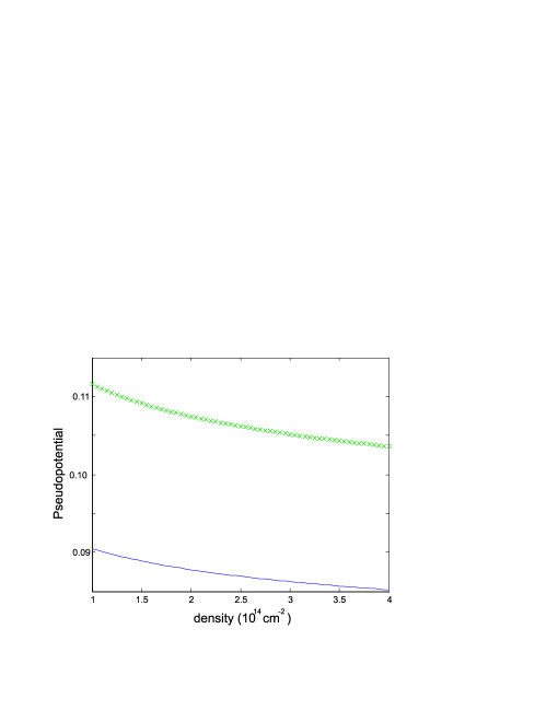
Figure 1: (Color online) Pseudopotentials $\mu_{11}$ (blue line) and $\mu_{12}$ (green crosses) as function of the charge carrier density $n$.

Calculation of the numerical values of the electron-phonon coupling constant $\lambda$ is more difficult because one has to know exact values of the matrix elements of the electron-phonon interaction. At the same time, the electron-phonon coupling $\lambda$ determines the self-energy of the electron-phonon interaction and can be extracted from photoemission studies. Therefore, we simply take this value from literature.

For a long time, there has been a rather poor agreement between theoretical results obtained using the local density approximation (LDA) and experimental values concerning the total coupling strength and the ratio between the two nonequivalent coupling parameters. The electron-phonon coupling is also sensitive to the substrate (For details, see Ref. [Bianchi, ] and citations therein).

A possible source of the disagreement has been identified in a recent paper, siegel where a copper substrate substantially screening the electron-electron Coulomb interaction was used and the agreement between the theoretical results calandra and the photoemission experiment was found. Both the theory and the experiment with the copper substrate lead to quite low values of the electron-phonon coupling constant $\lambda$ that remain below $0.05$ for electron densities up to $10^{14}\mathrm{cm}^{-2}$. Using the metallic substrate one should assume that the dielectric permeability of the substrate $\kappa$ entering Eq. (10) is a non-trivial function of the momentum. In order to avoid additional calculations for this system we note that even setting $\mu_{12}^{\ast}=0$, the values $\lambda<0.05$ can not provide superconductivity with a noticeable transition temperature.

Measurements of the electron-phonon coupling in potassium-doped graphene on Ir$(111)$ substrate Bianchi have lead to the value $\lambda=0{.}28$ for a doping level of $\mu=1.29\ \mathrm{eV}$ (corresponding to the electron density $n\approx 1\times 10^{14}\mathrm{cm}^{-2})$. Such a value of $\lambda$ would lead to a rather high transition temperature. However, the authors of Ref. [siegel, ] argue that the assumption of the linear spectrum used in Ref. [Bianchi, ] leads to a considerably overestimation of $\lambda$ and expect lower values of this parameter corresponding to theoretical values of Ref. [calandra, ].

The authors of Ref. [calandra, ] suggest the following formula for the function $\lambda\left(\mu\right)$ describing the dependence of the electron-phonon coupling on the chemical potential:

$$\lambda\left(\mu\right)=5.55C\sqrt{n}10^{-9}\mathrm{cm}$$ (72)

where $n$ is the number of electrons per surface area depending on $\mu$ via $\mu=\sqrt{\pi n}$ and $C=1$.

This formula gives for $n=1\times 10^{14}\mathrm{cm}^{-2}$ the value $\lambda=0.056$, which perfectly agrees with the experimental results of Ref. [siegel, ] for graphene on the metallic substrate.

However, angle-resolved photoemission spectroscopy (ARPES) experiments chesney1 ; bostwick ; chesney2 performed on doped graphene grown epitaxially on SiC lead to considerably higher values of $\lambda$. Larger values of the coupling constants obtained for graphene on other substrates mean that the unscreened Coulomb interaction renormalizes the electron-phonon interaction enhancing the latter. This conclusion correlates with the results of Ref. [basko, ], where an enhancement of the intervalley electron-electron coupling constant $\lambda_{12}$ was predicted. So, we can try to use the values of the coupling constant $\lambda$ obtained for such a non-metallic substrate.

According to a detailed analysis presented in Ref. chesney2, , the value of the coupling constant is $3.5-5$ times larger than predicted theoretically calandra , which apparently implies that the coefficient $C$ in Eq. (72) should take the values $C\sim 3.5-5$. The dielectric permeability of SiC equals $\kappa\approx 3{.}8$. park

As the constants $C$ somewhat vary depending on the method of their calculation and the pseudopotential $\mu_{12}^{\ast}$ depends on the substrate, we simply draw in Fig. 2 the dependence of the critical temperature $T_{c}^{inter}$ on the electron density $n$ for several values of $C$ and $\kappa$ using Eqs. (58, 59, 72).

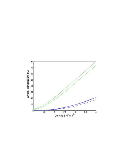
Figure 2: (Color online) Critical temperature calculated with Eq. (59). The curves show $T_{c}$ as function of the electron density $n$. Solid lines correspond to $\kappa=2.5$ while dashed lines are curves for $\kappa=3.8$. The bottom blue lines correspond to $C=3.5$ and the top green lines to $C=5.$

One can see from Fig. 2 that the superconductivity is possible for realistic parameters characterizing the system and the transition temperature $T_{c}^{inter}$ grows with increasing the electron density in graphene. Using the maximal possible value for $C$, $T_{c}$ becomes very high reaching the value of $70\ \mathrm{K}$ for very high electron densities. This value of the critical temperature is apparently too high, otherwise it would have been observed in the experiment. efetov Therefore, the value $C=5$ does not look realistic. At the same time, the value $C=3.5$ leads already to noticeable values of $T_{c}$.

The analysis presented above was done assuming that the chemical potential $\mu$ is far away from the Dirac points but is not close to the VHS. According to Ref. [chesney1, ], when approaching the VHS, the electron-phonon coupling $\lambda$ grows very fast, which would further increase the chances for the superconducting pairing. However, the linear-band estimation method used in Ref. [chesney1, ] was shown to overstate the coupling,park and the growth of the coupling $\lambda$ near VHS obtained in the latter publication was very slow reaching the value $\lambda\approx 0.22$. This value would still be sufficient for obtaining superconductivity with a reasonable critical temperature [see Eqs. (59)].

Unfortunately, the experiments Bianchi ; siegel ; chesney1 ; bostwick ; chesney2 have not been supplemented by transport experiments on the same materials at low temperatures, and it is not clear whether the samples studied could be superconducting at low temperatures, or not. At the same time, the superconductivity has not been observedefetov in the transport measurements on graphene with SiO₂ substrate for the electron density $n$ up to $4\times 10^{14}\mathrm{cm}^{-2}$ and more efforts should be expended to clarify the situation.

VI Discussion

In this work, we estimated the superconducting transition temperature for graphene as a function of the chemical potential $\mu$ or area electron density $n$. We considered the case when the chemical potential is far away from the Dirac point, which corresponds to very high electron density $n.$ At the same time, we assumed that the chemical potential $\mu$ is not in the vicinity of the VHS.

Starting with a model describing the electron-phonon and Coulomb interactions, we derived the Eliashberg equations for this system. Considering both anomalous and normal self-energies, we have obtained explicit formulas for the superconducting critical temperature that can be used not only for a weak electron-phonon coupling $\lambda$, but also for $\lambda$ of order $1$. We show that the Coulomb interaction in graphene is not very strong at high electron densities and does not necessarily destroy the superconducting pairing.

As the parameters entering Eq. (59) are not precisely known, we have drawn several curves in Fig. 2 corresponding to different values. It is clear that the critical temperature rather weakly depends on the dielectric permeability of the substrate and other details characterizing the Coulomb interaction. At the same time, the dependence on the electron-phonon coupling is strong, and we have shown curves corresponding to different values of these constants that may be considered as realistic.

By estimating the pseudopotentials $\mu^{\ast}$ describing the Coulomb interaction and using values of the electron-phonon coupling $\lambda$ extracted from photoemission experiments, we come to the conclusion that the transition temperature of the intervalley pairing $T_{c}^{inter}$ can reach values exceeding $10\ \mathrm{K}$ for sufficiently high electron area density $n$.

We have considered intra-and intervalley superconducting pairing and demonstrated that the intervalley pairing is more favorable. Effect of disorder on the intervalley superconductivity is weak but already a moderate concentration of impurities can destroy the intravalley pairing. All this means that the possibility of the intravalley pairing can be discarded in realistic situations.

According to previous findings, the coupling constant $\lambda$ can be considerably reduced provided a metallic substrate is used, which makes the superconductivity improbable in such systems.

Intercalating graphene by various materials may lead to an additional source of attraction between electrons and increase of the superconducting transition temperature.

The superconductivity becomes even more favorable when approaching the VHS. This is clear from the theoretical point of view because the density of states diverges at this point, which should lead to a considerable increase of $\lambda.$ The region of electron densities of order $10^{14}cm^{-2}$ is apparently already rather close to the VHS. This would imply that the approximation of the linear spectrum is no longer applicable. At the same time, the Fermi velocity decreases when approaching the VHS, leading to an additional increase of the density of states and, hence, of the critical temperature $T_{c}$.

A slow growth of the electron-phonon coupling near the VHS obtained in Ref. [park, ] using non-crossing self-energy diagrams indicates that this divergency is missed in this calculation. Moreover, using only non-crossing electron-phonon diagrams is not legitimate near the VHS and, therefore, the analysis of Ref. [park, ] is incomplete.

Provided the electron-phonon interaction grows and the interaction remains essentially attractive one should expect at the VHS the conventional $s$-wave singlet superconductivity with a sufficiently high transition temperature. By analyzing logarithmically diverging diagrams with the help of renormalization-group equations, a new type of unconventional (chiral) superconductivity was predicted recentlychubukov ; thomale in the situation when the interaction is repulsive. All this means that superconductivity in graphene at high electron density is very probable and we hope that it will be observed experimentally in the nearest future.

Strictly speaking, superconductivity with the identically zero resistance is not possible in $2D$ due to fluctuations of the order parameter and a finite energy required for generation of vortices. The transition temperature $T_{c}$ has been calculated in this work in the mean-field approximation neglecting the fluctuations and vortices, and this is not justified.

In practice, this means, however, that, instead of a sharp transition typical for $3D$ superconductors, one would observe a slower decay of the resistivity, which would make the transition rather broad. Although the resistivity does not become exactly zero in such a superconducting state, its value can be extremely small and not distinguishable from zero in real experiments.

VII Acknowledgements

We thank D.K. Efetov for useful discussions and acknowledge a financial support of Transregio 12 of DFG.

References

- (1) K.S. Novoselov, A.K. Geim, S.V. Morozov, D. Jiang, Y. Zhang, S.V. Dubonos, I.V. Grigorieva, and A.A. Firsov, Science 306, 666 (2004).
- (2) K.S. Novoselov, A.K. Geim, S.V. Morozov, D. Jiang, M.I. Katsnelson, I.V. Grigorieva, S.V. Dubonos, and A.A. Firsov, Nature 438, 197 (2005).
- (3) Y. Zhang, Y.-W. Tan, H.L. Stormer, and P. Kim, Nature 438, 201 (2005).
- (4) A.H. Castro Neto, F. Guinea, N.M.R. Peres, K.S. Novoselov, and A.K. Geim, Rev. Mod. Phys. 81, 109 (2009).
- (5) H.B. Heersche, P. Jarillo-Herrero, J.B. Oostinga, L.M.K. Vandersypen, and A. Morpurgo, Nature 446, 56 (2007).
- (6) B. Uchoa, and A.H. Castro Neto, Phys. Rev. Lett. 98, 146801 (2007).
- (7) N.B. Kopnin and E.B. Sonin, Phys. Rev. Lett. 100, 246808 (2008); Phys. Rev. B 82, 014516 (2010).
- (8) J.L. McChesney, A. Bostwick, T. Ohta, T. Seyller, K. Horn, J. Gonzalez, and E. Rotenberg, Phys. Rev. Lett. 104, 136803 (2010).
- (9) D.K. Efetov and P. Kim, Phys. Rev. Lett. 105, 256805 (2010).
- (10) J. Gonzalez, Phys. Rev B 78, 205431 (2008).
- (11) R. Nandkishore, L. Levitov, and A. Chubukov, arXiv: 1107.1903.
- (12) Maximilian Kiesel, Christian Platt, Werner Hanke, Dmitry A. Abanin, Ronny Thomale, arXiv:1109.2953.
- (13) Yu. Lozovik and A. Sokolik, Phys. Lett. A 374, 2785 (2010).
- (14) G. Savini, A.C. Ferrari, and F. Giustino, Phys. Rev. Lett. 105, 037002 (2010)
- (15) G.M. Eliashberg, Zh. Eksp. Teor. Fiz. 38, 966 (1960); 39, 1437 (1960) [Sov. Phys. JETP 11, 696 (1960); 12, 1000 (1961)].
- (16) P. Morel and P.W. Anderson, Phys. Rev. 125, 1263 (1962).
- (17) W.L. McMillan, Phys. Rev. 167, 331 (1968).
- (18) A.A. Abrikosov, L.P. Gorkov, and I.E. Dzyaloshinskii, Methods of Quantum Field Theory in Statistical Physics, Prentice Hall, New York (1963).
- (19) G. Grimvall, The Electron-Phonon Interaction in Metals, North Holland , Amsterdam (1980).
- (20) A.C. Ferrari, J.C. Meyer, V. Scardaci, C. Casiraghi, M. Lazzeri, F. Mauri, S. Piscanec, D. Jiang, K.S. Novoselov, S. Roth, and A.K. Geim, Phys. Rev. Lett. 97, 187401 (2006).
- (21) J. Yan, Y. Zhang, P. Kim, and A. Pinczuk, Phys. Rev. Lett. 98, 166802 (2007).
- (22) D.M. Basko and I.L. Aleiner, Phys. Rev. B 77, 041409 (2008).
- (23) E.H. Hwang and S. Das Sarma, Phys. Rev. B 75, 205418 (2007).
- (24) S.V. Vonsovsky, Yu. A. Izyumov, and E.Z. Kurmaev, Superconductivity in Transition Metals, Springer-Verlag, Berlin, Heidelberg (1982).
- (25) J. P. Carbotte and F. Marsiglio, in The Physics of Superconductors, edited by K. H. Bennemann and J. B. Ketterson, Springer-Verlag, Berlin (2003), p. 233.
- (26) I. L. Aleiner, K. B. Efetov, Phys. Rev. Lett. 97, 236801 (2006).
- (27) L. P. Gorkov, in The Physics of Superconductors, edited by K. H. Bennemann and J. B. Ketterson, Springer-Verlag, Berlin (2003), p. 347.
- (28) A.A. Abrikosov and L.P. Gorkov, Zh. Eksp. Teor. Fiz. 39, 1781 (1960) [Sov. Phys. JETP 12, 1243 (1961)]
- (29) M. Bianchi, E.D.L. Rienks, S. Lizzit, A. Baraldi, R. Balog, L. Hornekær, and Ph. Hofmann, Phys. Rev. B 81, 041403(R), (2010).
- (30) D.A. Siegel, C.G. Hwang, A.V. Fedorov, and A. Lanzara, arXiv:1108.2566
- (31) M. Calandra and F. Mauri, Phys. Rev. B 76, 205411 (2007).
- (32) J.L. McChesney, A. Bostwick, T. Ohta, K.V. Emtsev, T. Seyller, K. Horn, and E. Rotenberg, arXiv:0705.3264
- (33) A. Bostwick, T. Ohta, J.L. McChesney, T. Seyller, K. Horn, and E. Rotenberg, Sol. St. Commun. 143, 63 (2007).
- (34) J.L. McCheseny, A. Bostwick, T. Ohta, K.V. Emtsev, T. Seyller, K. Horn, and E. Rotenberg, arXiv:0809.4046
- (35) C.-H. Park, F. Giustino, J.L. McChesney, A. Bostwick, T.Ohta, E. Rotenberg, M.L. Cohen, and S.G. Louie, Phys. Rev. B 77, 113410 (2008).