Mass conserved elementary kinetics is sufficient for the existence of a non-equilibrium steady state concentration

Abstract

Living systems are forced away from thermodynamic equilibrium by exchange of mass and energy with their environment. In order to model a biochemical reaction network in a non-equilibrium state one requires a mathematical formulation to mimic this forcing. We provide a general formulation to force an arbitrary large kinetic model in a manner that is still consistent with the existence of a non-equilibrium steady state. We can guarantee the existence of a non-equilibrium steady state assuming only two conditions; that every reaction is mass balanced and that continuous kinetic reaction rate laws never lead to a negative molecule concentration. These conditions can be verified in polynomial time and are flexible enough to permit one to force a system away from equilibrium. In an expository biochemical example we show how a reversible, mass balanced perpetual reaction, with thermodynamically infeasible kinetic parameters, can be used to perpetually force a kinetic model of anaerobic glycolysis in a manner consistent with the existence of a steady state. Easily testable existence conditions are foundational for efforts to reliably compute non-equilibrium steady states in genome-scale biochemical kinetic models.

Keywords: thermodynamic forcing, chemical reaction network, stoichiometric consistency.

1 Introduction

There are various approaches for simulation of biochemical network function [19]. In principle, an ideal approach would accurately represent known physicochemical principles of reaction kinetics, tailored with kinetic parameters specific to a particular organism. However, when modeling genome-scale biochemical networks, one’s choice of modeling approach is also shaped by concerns of computational tractability. One of the main reasons that flux balance analysis [36, 11, 31, 24, 23] has found widespread applications in genome-scale modeling is that the underlying algorithm is typically based on linear optimization. In general, industrial quality software implementations of linear optimization algorithms are guaranteed to find an optimal solution, if one exists, or otherwise give a certificate that the problem posed is infeasible. In the process of iterative model development, one may use flux balance analysis to test if a stoichiometric model, obtained from a draft reconstruction, actually admits a steady state flux (reaction rate) [33]. If not, various algorithms have been developed that help to detect missing reactions [33] or stoichiometric inconsistencies [14] (discussed further in Section 2.1).

Flux balance analysis predicts fluxes that satisfy steady state mass conservation but not necessarily energy conservation or the second law of thermodynamics [4, 27, 13]. Whilst the set of steady state mass conserved fluxes includes those that are thermodynamically feasible, additional constraints are required in order to guarantee a flux that additionally satisfies energy conservation and the second law of thermodynamics [12]. Within the set of steady state fluxes that satisfy mass conservation, energy conservation and the second law of thermodynamics, there is a subset that additionally satisfy various reaction kinetic rate laws [8]. The satisfaction of such kinetic constraints is important for accurate representation of various biochemical processes where the abundance of a molecule affects the rate of a reaction, e.g., allosteric regulation [16, 18].

There are various algorithmic barriers to genome-scale kinetic modeling that preclude satisfaction of all of the aforementioned thermodynamic and kinetic constraints, without resorting to rate law approximation. Apart from the open algorithmic challenge to develop an algorithm for efficient computation of thermodynamically and kinetically feasible steady states in genome-scale kinetic models, there is also the challenge of mathematically expressing the necessary and sufficient conditions for existence of such a steady state in a manner that can be efficiently tested given a genome-scale model.

The quantitative study of chemical reaction kinetics has a long history, beginning perhaps with Ludwig Wilhemy’s 1850 discovery that the rate of a chemical reaction is proportional to the concentrations of consumed substrates [39]. This fundamental law of chemical kinetics is well known to chemists and biochemists alike. However, due to imperfect inheritance of knowledge, there are other useful facts, established generations ago, that are slipping from the consciousness of chemists and biochemists alike - as measured by contemporary citations. Even for a multifaceted paper with many citations, those citations can be due to a historically facet, not necessarily the most useful facet in a contemporary sense. A case in point is the 1962 paper by James Wei entitled “Axiomatic treatment of chemical reaction systems” [37]. This excellent paper has been cited 65 times, but only twice in the last 10 years and infrequently by theoretical biochemists. The vast majority of citations refer to Wei’s treatment of the stability of chemical reaction systems with Lyapunov functions. Exceptionally, the importance of Wei’s result, concerning the conditions for existence of non-equlibrium steady states, is realized, e.g., in 1976 Perelson used Wei’s result to illustrate the danger inherent in concluding results from mathematical models of systems of chemical reactions that do not conserve mass [25].

Herein we build upon Wei’s work that establishes sufficient conditions for the existence of at least one steady state reaction flux and molecule concentration for a broad class of chemical kinetic models. This class of kinetic model includes all those networks with exclusively mass balanced chemical reactions, where the kinetics rate laws are such that molecule concentration can never be a negative quantity. This class of reaction network includes all biochemical reaction networks. The conditions for existence may be easily tested by a trivial check on the kinetic rate law formulation for each reaction, together with a test of stoichiometric consistency using linear optimization [14].

In Section 2 we introduce some mathematical definitions of pertinent chemical reaction network concepts. Section 3 states and proves theorem concerning the existence of a non-negative steady state molecule concentration (vector) for mass conserved elementary reaction kinetics. This theorem and proof follow the more general case outlined in broad strokes by Wei [37]. Based on citation history, Wei’s result seems to be lost upon the biochemical modeling community. In Section 4, we illustrate for the first time, the utility of Wei’s existence theorem for modeling non-equlibrium steady states with various examples, including a kinetic model of anaerobic glycolysis in Trypanosoma brucei. Finally we summarise and attempt to place this work in the context of established mathematical approaches to model biochemical reaction networks.

2 Chemical reaction networks

2.1 Stoichiometry

Consider a biochemical network with $m$ molecules and $n$ elementary reactions. An elementary reaction is one for which no reaction intermediates have been detected or need to be postulated in order to describe the chemical reaction on a molecular scale. It follows that the reaction stoichiometry is sufficient to define the molecularity of the molecules involved in the reaction. One may combine elementary reactions together to form a composite reaction. One can define the topology of the resulting hypergraph using a generalized incidence matrix, $\mathbf{S}\in\mathbb{\mathbb{Z}}^{m,n}$, where $\mathbf{S}$ is always singular and typically $r\equiv\textrm{rank}(\mathbf{S})<m<n$ for large biochemical networks. Each row in this stoichiometric matrix represents a particular molecule, e.g., glucose, whilst each column represents a reversible biochemical reaction. We assume that all biochemical reactions are indeed reversible [20]. For each reversible reaction, convention dictates one direction be designated forward and the other reverse. With respect to the forward direction, for all $i=1\ldots m$ and $j=1\ldots n$, $S_{ij}<0$ if molecule $i$ is a substrate in a reaction, meaning that it is consumed by the reaction $j$, $S_{ij}>0$ if molecule $i$ is a product, meaning that it is produced by a reaction, and $S_{ij}=0$ otherwise. Typically stoichiometric coefficients are integers reflecting the whole number molecularity for a molecule consumed or produced in a reaction.

Each column of a stoichiometric matrix contains at least one negative coefficient and one positive coefficient, reflecting either the chemical conversion of one molecule to another, or in multi-compartmental models, the transport of a molecule from one compartment to another, i.e., a transport reaction may consume one molecule in a reactant compartment and produces one molecule in a different product compartment, even if the molecule is physically identical. We assume that each column of $\mathbf{S}$ corresponds to one mass conserving chemical reaction. A necessary, but insufficient condition for mass balancing is that each column of $\mathbf{S}$ must have at least one positive coefficient and at least one negative coefficient. We say that a chemical reaction is $linear$ when the corresponding column of $\mathbf{S}$ contains two nonzero coefficients, $\{-1,1\}$. We say that a chemical reaction is $bilinear$ when the corresponding column of $\mathbf{S}$ contains three non-negative coefficients, $\{-1,1,1\}$ or $\{-1,-1,1\}$. There may be more than one negative (positive) coefficient in a column when a reaction involves more than one substrate (product). In reaction networks with composite reactions, nonzero stoichiometric coefficients are typically not of magnitude one. However, even the most complicated composite reaction can be decomposed into linear and bilinear reactions.

Each row of $\mathbf{S}$ contains at least one positive coefficient and at least one negative coefficient, reflecting the requirement for at least one reaction to produce and at least one reaction to consume each molecule. A stoichiometric matrix for a chemical reaction network is said to be consistent if each molecule can be assigned a single positive molecular mass, without violating mass conservation, and inconsistent otherwise [14, 10]. Mathematically, this translates to the existence of at least one strictly positive vector, $\mathbf{m}\in\mathbb{R}_{>0}^{m}$, in the left nullspace of a consistent stoichiometric matrix $\mathbf{S}^{T}\cdot\mathbf{m}=\mathbf{0}$. Strictly, we could say that each row of $\mathbf{S}$ corresponds to an isotopically distinct molecular entity in order that the corresponding molecular mass be precisely defined, as two otherwise identical molecules can have different molecular mass depending on their isotopic label e.g. ${}^{13}\textrm{C}$ vs ${}^{14}\textrm{C}$ glucose. However, we shall assume that reaction kinetic parameters are isotopomer invariant so we need not be so strict.

2.2 Reaction kinetics

Perhaps the simplest reaction kinetic assumption is that a unidirectional reaction rate is proportional to the product of the concentrations of each substrate consumed [39]. Let us define forward and reverse stoichiometric matrices, $\mathbf{F},\mathbf{R}\in\mathbb{R}_{\geq 0}^{m,n}$ respectively, where $\mathbf{F}_{ij}$ denotes the stoichiometry of substrate $i$ in forward reaction $j$ and $\mathbf{R}_{ij}$ denotes the stoichiometry of substrate $i$ in reverse reaction $j$. It follows that the stoichiometric matrix is defined by $\mathbf{S}\equiv-\mathbf{F}+\mathbf{R}$. It is possible for the same molecule to appear as both a substrate and a product in the same unidirectional reaction, e.g., an auto-catalytic reaction, so it is natural to define $\mathbf{S}$ in terms of $\mathbf{F}$ and $\mathbf{R}$, rather than the other way around. We we may now express elementary kinetics for forward and reverse reaction rates, respectively $\mathbf{v}_{f},\mathbf{v}_{r}\in\mathbb{R}^{n}$, as

$$\begin{array}[]{cc}\mathbf{v}_{f}(\mathbf{k}_{f},\mathbf{x})\equiv\textrm{diag}(\mathbf{k}_{f})\cdot\exp(\mathbf{F}^{T}\cdot\ln(\mathbf{x})),\\ \mathbf{v}_{r}(\mathbf{k}_{r},\mathbf{x})\equiv\textrm{diag}(\mathbf{k}_{r})\cdot\exp(\mathbf{R}^{T}\cdot\ln(\mathbf{x})),\end{array}$$ (1)

where we assume non-negative elementary kinetic parameters $\mathbf{k}_{f},\mathbf{k}_{r}\in\mathbb{R}_{\geq 0}^{n}$, and the exponential or natural logarithm of a vector is meant component-wise . We say that a pair of forward and reverse elementary kinetic parameters are thermodynamically feasible when they satisfy

$$\exp\left(-\mathbf{S}_{j}^{T}\cdot\frac{\mathbf{u}^{\circ}}{RT}\right)=\frac{k_{f,j}}{k_{r,j}},$$ (2)

where $\mathbf{u}^{o}\in\mathbb{R}^{m}$ is a vector of standard chemical potentials, $R$ is the gas constant and $T$ is temperature. Thermodynamically feasible kinetic parameters for all reactions implies detailed balance at thermodynamic equilibrium, i.e., $\mathbf{v}_{f}=\mathbf{v}_{r}$ [35].

We refer to (1) as mass action kinetics [28] only after we have stated our assumption that (2) also holds for each mass conserving reversible reaction. In the words of Horn & Jackson [17] “a kinetic description of chemical reactions in closed systems with ideal mixtures, completely consistent with the requirements of stoichiometry and thermodynamics, may be obtained by satisfying the following four conditions”:

• The rate function of each elementary reaction is of the mass action form.

• The stoichiometric coefficients are such that mass is conserved in each elementary reaction.

• The kinetic constants in the rate functions are constrained in such a way that the principle of detailed balancing is satisfied.

• The stoichiometric coefficients are non-negative integers.

Condition (a) is represented by (1) and conditon (b) is satisfied by strict adherence to elemental balancing for each reaction during network reconstruction [33, 34]. Horn & Jackson [17] considered general mass action kinetics when only (a) was assumed to hold. We shall consider mass conserved elementary kinetics where (a) and (b) are assumed to hold but (c) and (d) are allowed to be relaxed for a subset of reactions. We shall return to this point in the discussion. We take the dynamical equation for mass conserved elementary kinetics to be

$$\dot{\mathbf{x}}\equiv\frac{d\mathbf{x}}{dt}=\mathbf{S}\cdot(\mathbf{K}_{f}\cdot\exp(\mathbf{F}^{T}\cdot\ln\left(\mathbf{x}\right))-\mathbf{K}_{r}\cdot\exp(\mathbf{R}^{T}\cdot\ln\left(\mathbf{x}\right)))$$ (3)

where $t$ denotes time, all reactions conserve mass, all reactions are reversible, $\mathbf{K}_{f}=\textrm{diag}(\mathbf{k}_{f})$, $\mathbf{K}_{r}=\textrm{diag}(\mathbf{k}_{r})$ and $\mathbf{k}_{f},\mathbf{k}_{r}\in\mathbb{R}_{\geq 0}^{m}$.

2.3 Concentration non-negativity

Figure 1: Conceptual illustration of the Brouwer fixed point theorem in one dimension. An arbitrary continuous function $f$ is represented by the graph mapping the abscissa to the ordinate. On the abscissa, the bounded interval between zero and one represents the domain. The domain is closed as it includes its endpoints and is convex as every line interval is a convex set. The interval between zero and one on the ordinate represents the codomain of $f$. The image of $f$ is a continuous interval contained within the codomain of $f$, so $f$ is into. It is unnecessary for $f$ to be onto. The diagonal line represents equality of the values in the domain and codomain. Tracing a continuous curve from left to right, between the dots, we see that it must intersect the diagonal at some point. At the point where the diagonal meets the curve, the value of the domain equals the value of the image $x^{*}=x^{\prime}=f(x)$. When the value passed into the function is the same as the value passed out by the function, this value is termed a fixed point. (Figure adapted from http://commons.wikimedia.org/wiki/File:Fixedpoint1d.svg)

Physically, one would expect that molecular concentration be a non-negative quantity. Starting from an initial non-negative concentration, $\mathbf{x}_{0}\geq 0$, it has been proven mathematically that all subsequent concentrations are non-negative when the evolution of a system is subject to elementary reaction kinetics [5, 7]. Elementary kinetics is essentially non-negative if, for all $i=1\ldots m$, $\dot{x_{i}}\geq 0$ for all $x_{i}\in\mathbb{R}_{\geq 0}$, where $\dot{x_{i}}$ and $x_{i}$ denote the $i^{th}$ component of $\dot{\mathbf{x}}$ and $\mathbf{x}$, respectively. This mathematical formulation can be easily be chemically interpreted. Suppose the concentration of molecule A is zero; then irrespective of what the non-negative concentration is for all other molecules, the rate of change in concentration for molecule A is non-negative. To understand why, recall that in elementary kinetics the rate of a unidirectional reaction is always the product of a non-negative elementary kinetic parameter and the concentration(s) of the substrate(s), each to the power of the absolute value of the corresponding stoichiometric coefficient. If a molecule’s concentration is zero then all reactions consuming that molecule have a rate of zero; hence, there can be no consumption of that molecule and its rate of change in concentration is non-negative.

Consider the chemical reaction network with the single reaction

$$A\overset{k_{f}}{\underset{k_{r}}{\rightleftharpoons}}B+C.$$

Let the forward and reverse reaction rates be given by elementary kinetics $v_{f}=k_{f}a$ and $v_{r}=k_{r}bc$ with $k_{f},k_{r}\in\mathbb{R}_{\geq 0}$, where lowercase refers to concentration of the corresponding uppercase molecule. If the initial concentrations of all molecules are non-negative it is impossible for any molecule’s concentration to go negative because $a=0$ implies $v_{f}=0$ so no consumption of $A$ would occur and therefore $a$ cannot be negative. Observe that the conditions for concentration non-negativity place no constraints on the ratio of forward over reverse kinetic parameter, but only that all kinetic parameters be non-negative.

A further technical restriction is that $\dot{\mathbf{x}}$ be given by a locally Lipschitz continuous function, but this is easily satisfied by deterministic formulations of kinetics where the corresponding differential equations are continuously differentiable (Lemma 1, [7]). Starting from an initial non-negative concentration, equation (3) constrains all subsequent concentrations to be non-negative as we assume elementary reaction kinetics with non-negative kinetic parameters. Even for non-negative but thermodynamically infeasible kinetic parameters, which violate (2), it is true that if one begins with non-negative initial concentrations then all subsequent concentrations remain non-negative.

3 Existence of a steady state for mass conserved elementary kinetics

The following theorem establishes sufficient conditions for existence of a steady state concentration for a dynamical system governed by mass conserved elementary kinetics.

Theorem 1.

Let the dynamical equation for mass conserved elementary kinetics be

$$\dot{\mathbf{x}}\equiv\frac{d\mathbf{x}}{dt}=\mathbf{S}\cdot(\mathbf{K}_{f}\cdot\exp(\mathbf{F}^{T}\cdot\ln\left(\mathbf{x}\right))-\mathbf{K}_{r}\cdot\exp(\mathbf{R}^{T}\cdot\ln\left(\mathbf{x}\right)))$$ (4)

where $\mathbf{x}\equiv\mathbf{x}(t)\in\mathbb{R}^{m}$ is molecule concentration at time $t>0$, $\dot{\mathbf{x}}\in\mathbb{R}^{m}$ is the time derivative of concentration, $\mathbf{K}_{f}=\textrm{diag}(\mathbf{k}_{f})$, $\mathbf{K}_{r}=\textrm{diag}(\mathbf{k}_{r})$ and $\mathbf{k}_{f},\mathbf{k}_{r}\in\mathbb{R}_{\geq 0}^{n}$ are non-negative forward and reverse kinetic parameters. $\mathbf{F},\mathbf{R}\in\mathbb{R}_{\geq 0}^{m,n}$ are forward and reverse stoichiometric matrices. $\mathbf{S}\equiv-\mathbf{F}+\mathbf{R}$ is a consistent stoichiometric matrix defined by the existence of at least one strictly positive vector $\mathbf{m}\in\mathbb{R}_{>0}^{m}$, such that $\mathbf{S}^{T}\cdot\mathbf{m}=\mathbf{0}$. Assuming a strictly positive initial concentration $\mathbf{x}_{0}\equiv\mathbf{x}(0)\in\mathbb{R}_{>0}^{m}$, then there exists at least one non-negative steady state concentration $\mathbf{x}_{\geq 0}^{\star}$, such that $\dot{\mathbf{x}}=\mathbf{0}$.

Proof.

We define the function $\mathbf{f}(\mathbf{x})\,:\,\mathbb{R}^{m}\rightarrow\mathbb{R}^{m}$

$$\mathbf{f}(\mathbf{x}) = \mathbf{x}+\dot{\mathbf{x}}$$ (5)

where $\mathbf{f}(\mathbf{x})\equiv\mathbf{x}(t+\tau)$ represents the concentration after an arbitrary small time interval $\tau>0$. If it exists, a fixed point $\mathbf{x}^{\star}$, such that $\mathbf{f}(\mathbf{x}^{\star})=\mathbf{x}^{\star}$, corresponds to a steady state concentration, $\mathbf{x}^{\star}(t)=\mathbf{x}^{\star}(t+\tau),$ or equivalently $\dot{\mathbf{x}}=0$. Observe that $f(\mathbf{x})$ is continuous as $\dot{\mathbf{x}}$ is given by a continuous function. Let us define the closed, bounded and convex set

$$\Omega=\left\{\mathbf{x}\geq 0,\;\mathbf{m}^{T}\cdot\mathbf{x}=\mathbf{m}^{T}\cdot\mathbf{x}_{0}>0\right\},$$

as the domain of $\mathbf{f}(\mathbf{x})$. For a strictly positive initial concentration vector, then elementary kinetics, continuity of $\mathbf{f}(\mathbf{x})$ and non-negative kinetic parameters are sufficient conditions to ensure that all subsequent concentrations are non-negative, $\mathbf{f}(\mathbf{x})\geq 0$ (Theorem 2, [7]). Since $\mathbf{S}\in\mathbb{R}^{m,n}$ is a stoichiometrically consistent matrix there exists an $\mathbf{m}\in\mathbb{R}_{>0}^{m}$ such that $\mathbf{m}^{T}\cdot\mathbf{S}=0$ and therefore $\mathbf{m}^{T}\cdot\dot{\mathbf{x}}=0$. It follows that $\mathbf{m}^{T}\cdot\mathbf{f}(\mathbf{x})=\mathbf{m}^{T}\cdot\mathbf{x}_{0}$ for all $\mathbf{x}\in\Omega$. This together with the non-negativity of $\mathbf{f}(\mathbf{x})$ establishes that $\mathbf{f}(\mathbf{x})\in\Omega$. We have now established that $\mathbf{f}(\mathbf{x})$ is a continuous mapping from a closed, bounded and convex set into itself. By Brouwer’s fixed point theorem there exists at least one fixed point $\mathbf{f}(\mathbf{x}^{\star})=\mathbf{x}^{\star}$ and therefore there exists at least one steady state. ∎

In the proof of existence of steady states for mass conserved elementary kinetics, we make use of the following theorem that we state without proof.

Theorem 2.

(Brouwer fixed point theorem). Let $\Omega$ be a closed, bounded and convex set in $\mathbb{R}^{m}$, and let $\Phi:\mathbb{R}^{m}\rightarrow\mathbb{R}^{m}$ be a function that is continuous on $\Omega$ and maps $\Omega$ into itself. Then there exists a point $\mathbf{x}\in\Omega$ such that $\Phi(\mathbf{x})=\mathbf{x}$.

There is a voluminous literature on fixed point theory [15]. Figure 1 illustrates an intuitive appreciation for the rationale behind Brouwer’s fixed point theorem by considering a one dimensional case, that is, a function mapping of an interval on a line into itself.

4 Utility of steady state existence theorem

Theorem 1 is non-constructive in the sense that it does not describe an algorithm for computation of steady state concentrations. In the case where one is modeling a system of exclusively mass conserved reversible reactions with mass action kinetics, it has long been known that a unique steady state concentration can be computed with a single convex optimization problem [38]. Such a steady state corresponds to a thermodynamic equilibrium where detailed balance holds. The development of a reliable algorithm to compute non-equilibrium steady states for arbitrary large networks is an important open problem. In the process of algorithm development, it is essential to know, a priori, if at least one steady state exists. Otherwise it becomes impossible to distinguish if a failure to compute a steady state is due to a shortcoming of an algorithm’s design, or due to to an ill-posed problem without a solution in the first instance.

The key difference between an equilibrium and non-equilibrium steady state is that the latter is accompanied by thermodynamic forcing of the system by the environment. In chemical reaction networks, time invariant thermodynamic forcing has been mathematically represented by clamping a subset of concentrations away from equilibrium or injecting mass across the boundary of the model [29]. However, for kinetic modeling of time invariant concentrations, any formulation of a forced system must be compatible with the existence of at least one steady state concentration vector. It is therefore important to establish, if possible, the conditions for existence of at least one steady state for each formulation. Some formulations are actually incompatible with the existence of a steady state.

4.1 System forcing where a steady state may not exist

One approach to forcing a system is to represent the exchange of molecules between a system and its environment with a set of mass imbalanced source or sink reactions, respectively $\emptyset\rightarrow A$ and $A\rightarrow\emptyset$, where $A$ is an arbitrary molecule. Let $\mathbf{S}_{e}\in\mathbb{Z}^{m,k}$ denote the stoichiometry of mass imbalanced exchange reactions. To the author’s knowledge, for networks with bilinear reactions, no theorem exists that defines the conditions on the data $\{\mathbf{S},\mathbf{S}_{e},\mathbf{k}_{f},\mathbf{k}_{r}\}$ such that there still exists at least one non-equilibrium steady state. As described in Section 2.1, an augmented stoichiometric matrix, $\bar{\mathbf{S}}=[\begin{array}[]{cc}\mathbf{S}&\mathbf{S}_{e}\end{array}]$, containing mass imbalanced exchange reactions will not be stoichiometrically consistent, so Theorem 1 does not apply.

Another approach to forcing a system, in which all reactions are mass balanced, is to attempt to iterate toward a steady state of the forced dynamical system

$$\dot{\mathbf{x}}\equiv\frac{d\mathbf{x}}{dt}=\mathbf{S}\cdot(\mathbf{v}_{f}(\mathbf{k}_{f},\mathbf{x})-\mathbf{v}_{r}(\mathbf{k}_{r},\mathbf{x}))-\mathbf{b},$$ (6)

where $\mathbf{b}$ is a concentration invariant forcing vector in the range of the stoichiometric matrix, $\mathbf{b}\in\mathcal{R}(\mathbf{S})$. If one chooses a $\mathbf{b}^{\star}\in\mathcal{R}(\mathbf{S})$ such that

$$\mathbf{S}\cdot(\mathbf{v}_{f}(\mathbf{k}_{f},\mathbf{x}^{\star})-\mathbf{v}_{r}(\mathbf{k}_{r},\mathbf{x}^{\star}))=\mathbf{b}^{\star}$$ (7)

is satisfiable, then this would correspond to forcing in a manner independent of molecule concentration. Given $\mathbf{x}^{\star}$ it is trivial to compute $\mathbf{b}^{\star}$ but not the other way around. If we assume that unidirectional reaction rates are as defined in (1) and (2), then by rearrangement, one may express (3) as

$$\dot{\mathbf{x}}=[\begin{array}[]{cc}\mathbf{S}&-\mathbf{S}]\end{array}\cdot\textrm{diag}(\left[\begin{array}[]{c}\mathbf{k}_{f}\\ \mathbf{k}_{r}\end{array}\right])\cdot\exp([\begin{array}[]{cc}\mathbf{F}&\mathbf{R}\end{array}]^{T}\cdot\ln\left(\mathbf{x}\right)),$$

where $[\begin{array}[]{cc}\mathbf{F}&\mathbf{R}\end{array}]\in\mathbb{Z}^{m,2n}$. Typically $m<n$ and $\textrm{rank}([\begin{array}[]{cc}\mathbf{F}&\mathbf{R}\end{array}])<n$, so the image of $[\begin{array}[]{cc}\mathbf{F}&\mathbf{R}\end{array}]^{T}\cdot\ln\left(\mathbf{x}\right)$ is not the whole of $\mathbb{R}^{2n}$ and therefore the set of all $\dot{\mathbf{x}}$ is a subset of the range of the stoichiometric matrix. The set of $\mathbf{b}^{\star}$ such that (7) is satisfiable is only a subset of the range of the stoichiometric matrix, so a steady state may not necessarily exist for an arbitrary $\mathbf{b}$. Attempting to force a system with (6) leaves one with the problem of attempting an a priori choice of concentration invariant forcing vector that may not admit a steady sate concentration.

4.2 System forcing where a steady state must exist

Theorem 1 is constructive in the sense that it leads to a method to force a system in a manner that ensures there always exists at least one non-equilibrium steady state concentration vector. The key point is to recognise that Theorem 1 holds for any choice of non-negative kinetic parameters. Additional thermodynamic constraints on kinetic parameters (2) are optional on a per reaction basis. If all reversible reactions have thermodynamically feasible kinetic parameters, then the only steady state is thermodynamic equilibrium, but if at least one reversible reaction is modeled with thermodynamically infeasible kinetic parameters, that violate (2), then detailed balance does not hold but there always exists at least one non-equilibrium steady state.

It is not physicochemically realistic to model actual chemical reactions with thermodynamically infeasible kinetic parameters for any form of kinetic rate law [8]. However, one may include a mass balanced, reversible perpetireaction with thermodynamically infeasible kinetic parameters, purely for the modeling purpose of forcing a system away from equilibrium. (The prefix perpeti is from the latin perpes meaning lasting throughout, continuous, uninterrupted, continual, perpetual; see www.perseus.tufts.edu.). The augmentation of a consistent stoichiometric matrix with a mass balanced perpetireaction still retains the stoichiometric consistency of the augmented matrix. Assuming that elementary reaction kinetics is used to model each unidirectional reaction there will still exist a steady state. We now illustrate one choice of perpetireaction by considering a biochemical example.

4.2.1 Mass conserved elementary kinetics of Trypanosoma brucei

The utility of Theorem 1 can be illustrated by considering a typical kinetic modeling scenario, such as the modeling of anaerobic glycolysis in the African trypanosome, Trypanosoma brucei, the causative agent of human African trypanosomiasis [3, 1]. Based on a phenomenological kinetic model of T. brucei glycolysis [2] the stoichiometry of anaerobic glycolysis may be represented in skeleton form by the composite chemical reactions in Figure 2. Modeling composite reactions with elementary kinetic rate laws is pseudoelementary kinetics, but for the purpose of illustrating the utility of Theorem 1, this distinction is superfluous. Starting with extracellular glucose the overall stoichiometry of this pathway may be given by the mass balanced composite reaction

$$\textrm{glucose }\rightleftharpoons\textrm{glycerol + pyruvate }+H^{+}.$$ (8)

This composite reaction may be used as a perpetireaction that, in reverse, connects the outputs of anaerobic glycolysis back to the glucose input. This perpetireaction is the TrypGlycAner reaction in Figure 2. As perpetireaction kinetic parameters violate (2), no equilibrium steady state exists as detailed balance [35] is violated, but there exists at least one non-equilibrium steady state for the augmented system. Such a non-equilibrium steady state conserves mass in all reactions, and all except the perpetireaction conserve energy.

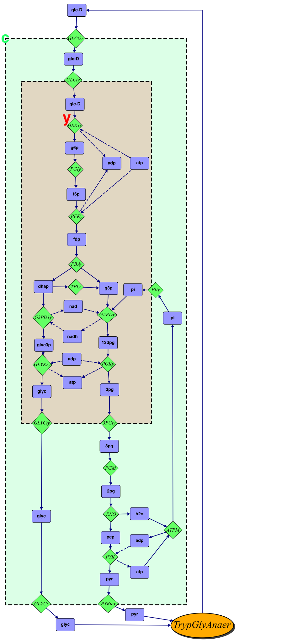
Figure 2: The anaerobic glycolysis pathway of Trypanosoma brucei, part of which is in the cytoplasm (c) and part of which is within a membrane-bounded, peroxisome-like organelle termed a glycosome (y). The input to this pathway is glucose (glc-D) and the outputs are glycerol (glyc), pyruvate (pyr) and hydrogen ion (not shown for clarity). For modeling purposes, one can construct a perpetual reaction, or perpetireaction (TrypGlycAner), from extracellular output metabolites to extracellular glucose input to form, with the anaerobic glycolysis pathway, a stoichiometrically balanced cycle. With appropriate choice of kinetic parameters, a non-equilibrium steady state concentration corresponds to net flux in the directions indicated by the arrows. Dashed arrows indicate the involvement of cofactors. (Illustration created with Omix [9].)

Assuming constant temperature and pressure, and uniform spatial concentrations within a single compartment, the existence of a single chemical potential for each (compartment specific) molecule is a necessary and sufficient condition for conservation of energy [26, 22, 30]. The violation of (2) by the pair of forward and reverse elementary kinetic parameters, $p_{f}$ and $p_{r}$, for the perpetireaction means that there exists no single standard chemical potential for each molecule and hence no single chemical potential for each molecule. With reference to the T. brucei example, one or more of glucose, glycerol, pyruvate or hydrogen ion can not be assigned a unique chemical potential. This is equivalent to the statement that the stoichiometrically weighted sum of chemical potential around the single stoichiometrically balanced cycle formed by the anaerobic glycolysis pathway and the perpetireaction is not zero [4, 13].

One can also think of the perpetireaction as a chemical reaction that extracts energy, but not molecular moieties, from an infinitely large source in the environment. In a non-equilibrium steady state, the amount of energy extracted from the environment per unit time by the perpetireaction is equal to the entropy production rate of all the other reactions. In analogy with electrical networks, at a non-equilibrium steady state, a perpetireaction acts like a direct current voltage source. Indeed, in the representation of electrical networks, even the most elementary circuit diagram forms a closed cycle with some voltage source in the loop to drive electrons around the circuit. In numerically calculated steady states the T. brucei model, if all thermodynamically feasible kinetic parameters are given a unit value and $p_{f}>p_{r}$ then the net steady state flux of anaerobic glycolysis proceeds in the usual direction (Figure 2). However, if $p_{f}<p_{r}$ then anaerobic glycolysis proceeds in the reverse direction. In an electrical network analogy, this switch is equivalent to reversing the polarity of a direct current voltage source.

4.2.2 More general examples

In Section 4.2.1, we considered an example where the overall system being modeled consisted of a single stoichiometrically balanced pathway. More precisely a single extreme ray of an augmented stoichiometric matrix

$$\overline{\mathbf{S}}=[\begin{array}[]{cc}\mathbf{S}&\mathbf{S}_{p}\end{array}]$$

where $\mathbf{S}_{p}$ is a column vector with reaction stoichiometry for a single composite perpetireaction, with net forward direction right to left in 8. In the general case of an arbitrary mass balanced stoichiometric matrix $\mathbf{S}\in\mathbb{R}^{m,n}$, then $\mathbf{S}_{p}\in\mathbb{R}^{m,k}$ can be an arbitrary set of $k$ column vectors, each of which could be a linear basis vector for the range of $\mathbf{S}$, accompanied by $k$ perpetireactions. In fact, any $\mathbf{b}\in\mathcal{R}(\mathbf{S})$ can be used to create an augmented stoichiometric matrix

$$\overline{\mathbf{S}}=[\begin{array}[]{cc}\mathbf{S}&-\mathbf{b}\end{array}]$$

that is still also consistent. Note however that this is not equivalent to forcing a system like 6 as the steady state $\mathbf{x}^{\star}$, that we know must exist, satisfies

$$0=[\begin{array}[]{cc}\mathbf{S}&-\mathbf{S}]\end{array}\cdot\textrm{diag}(\left[\begin{array}[]{c}\mathbf{k}_{f}\\ \mathbf{k}_{r}\end{array}\right])\cdot\exp([\begin{array}[]{cc}\mathbf{F}&\mathbf{R}\end{array}]^{T}\cdot\ln\left(\mathbf{x}^{\star}\right))-[\begin{array}[]{cc}\mathbf{b}&-\mathbf{b}\end{array}]\cdot\textrm{diag}(\left[\begin{array}[]{c}p_{f}\\ p_{r}\end{array}\right])\cdot\exp([\begin{array}[]{cc}\mathbf{b}_{f}&\mathbf{b}_{r}\end{array}]^{T}\cdot\ln\left(\mathbf{x}^{\star}\right)),$$

where $p_{f},p_{r}>0$ are perpetireaction parameters, with $\mathbf{b}_{f}\equiv\max(-\mathbf{b},0)$ and $\mathbf{b}_{r}\equiv\max(\mathbf{b},0)$ defined in an analogous manner to $\mathbf{F}$ and $\mathbf{R}$. Even more general is the consideration of continuous kinetic rate laws that guarantee concentration non-negativity. The same strategy to augment the system with perpetireactions, yet retain stoichiometric consistency, will yield a forced system where there always exists a steady state concentration vector.

5 Discussion

In the present work, Theorem 1 gives sufficient conditions for the existence of at least one non-negative steady state concentration vector, assuming elementary reaction kinetics for a set of mass balanced chemical reactions. All kinetic parameters are required to be positive but do not have to satisfy thermodynamic constraints (2) on the ratio of forward over reverse elementary kinetic parameter. Actual biochemical reactions are modeled with reactions that have thermodynamically feasible kinetic parameters. In order to conserve mass, yet admit a non-equilibrium steady state, one may augment the set of thermodynamically feasible reactions with one or more perpetireactions (perpetual reactions), defined as reactions with thermodynamically infeasible kinetic parameters. This gives the flexibility to model the non-equilibrium dynamics of a system closed to exchange of mass with the environment yet not isolated with respect to the exchange of energy with the environment. In a non-equilibrium steady state, the net input of chemical energy is the driving force for net flux through the stoichiometrically balanced system.

Theorem 1 does not preclude that a subset of molecule concentrations are actually zero at a steady state. There may exist more than one steady state and no conclusion can be drawn as to the stability or otherwise of the steady states that exist. Theorem 1 is non-constructive in that it does not provide an algorithm to compute a non-equilibrium steady state. However, Theorem 1 makes use of Brouwer’s fixed point theorem so, assuming the conditions required for Theorem 1 to hold, it may be possible to apply related constructive fixed point theorems [15] to design an algorithm that is guaranteed to converge to a non-equilibrium steady state. Contributions from fixed point theorists are encouraged and this is part of the reason for the detail in Section 2.1.

The sufficient conditions for existence of a non-equilibrium steady state are easily tested numerically for arbitrary large chemical networks [32]. As described in an elegant paper by Gevorgyan et al., [14] the stoichiometric consistency of a metabolic network can be proved or disproved by attempting the linear optimization problem

$$\underset{\textrm{{m}}}{\textrm{minimize}}\qquad \mathbf{e}^{T}\cdot\mathbf{m}$$ (9)

such that $$\mathbf{S}^{T}\cdot\mathbf{m}=\mathbf{0}$$ (10)

$$\mathbf{m}>\mathbf{0}$$ (11)

where $\mathbf{e}$ denotes a vector of ones and $\mathbf{S}\in\mathbb{Z}^{m,n}$ is a stoichiometric matrix. If there exists an $\mathbf{m}$ satisfying (10) and (11), then $\mathbf{S}$ is stoichiometrically consistent, otherwise a suitable solver will provide a certificate of infeasibility indicating that $\mathbf{S}$ is inconsistent. Alternatively, if one has rigorously applied mass balancing for each chemical reaction whilst reconstructing a network [33, 34], one will be able to assign a positive molecular mass corresponding to each of the molecules in the reconstruction. This strictly positive molecular mass vector satisfies (10) and (11), which is sufficient to conclude that the corresponding stoichiometric matrix is consistent.

The only other condition for Theorem 1 to hold is that continuous kinetic rate laws be formulated in a manner such that the concentration of any molecule can never be negative [7]. In this paper, we have framed Theorem 1 in terms of elementary reaction kinetics that satisfy concentration non-negativity if the elementary kinetic parameters are non-negative. However, one can envisage a more general version of Theorem 1 as there are many other continuous kinetic rate laws that satisfy concentration non-negativity [21]. Any continuous kinetic rate law, where the rate of a unidirectional reaction is non-negative and zero if and only if any of the concentrations of the molecules consumed in that reaction are zero [7], would form the conditions for a generalised version of Theorem 1. In any case, any phenomenological kinetic rate law can be derived from assumptions that allow simplification of a system of elementary chemical reactions [8]. As such, phenomenological kinetic modeling has its foundation in mass action kinetics.

6 Conclusion

It is 50 years since Wei’s Axiom’s on the existence of steady states for chemical reaction systems[37] and almost 40 years since Horn & Jackson [17] considered what they termed general mass action kinetics. In Horn & Jackson’s setting, elementary reaction rates are proportional to the abundance of the substrates involved in the reaction, each to the power of the absolute value of the corresponding stoichiometric coefficient. However, general mass action kinetics considers systems where kinetic parameters need not be thermodynamically feasible, stoichiometric coefficients need not be integers, and mass need not be conserved by each reaction. With regard to modeling chemical reaction networks, we agree that consideration of reactions with thermodynamically infeasible kinetic parameters does seem profitable for representing the perpetual forcing of a system, purely for modeling purposes. However, violation of mass conservation appears unnecessary, as a pair of thermodynamically infeasible kinetic parameters are sufficient to force a system away from equilibrium, and counterproductive, as the resulting system may not admit a non-equilibrium steady state. Horn & Jackson [17] do realize that the conditions for Wei’s existence result are unmet when mass is not conserved. We conclude that, rather than general mass action kinetics, assuming mass conserved elementary kinetics is sufficient for modeling non-equilibrium steady states in arbitrary large biochemical networks, as one is then sure that at least one steady state does actually exist. Similar conclusions hold for phenomenological kinetic modeling, .e.g., with Michaelis-Menten kinetics, as long as the continuos rate laws are such that concentration can never be negative.

References

References

- Bakker et al., [2010] Bakker, B. M., Krauth-Siegel, R. L., Clayton, C., Matthews, K., Girolami, M., Westerhoff, H. V., Michels, P. A. M., Breitling, R. & Barrett, M. P. 2010. The silicon trypanosome. Parasitology, 137 (9), 1333–1341.
- Bakker et al., [1997] Bakker, B. M., Michels, P. A., Opperdoes, F. R. & Westerhoff, H. V. 1997. Glycolysis in bloodstream form trypanosoma brucei can be understood in terms of the kinetics of the glycolytic enzymes. J Biol Chem, 272 (6), 3207–3215.
- Barrett et al., [2010] Barrett, M. P., Bakker, B. M. & Breitling, R. 2010. Metabolomic systems biology of trypanosomes. Parasitology, 137 (9), 1285–1290.
- Beard et al., [2002] Beard, D. A., Liang, S. & Qian, H. 2002. Energy balance for analysis of complex metabolic networks. Biophys J, 83 (1), 79–86.
- Bernstein & Bhat, [1999] Bernstein, D. S. & Bhat, S. P. 1999. Nonnegativity, reducibility, and semistability of mass action kinetics. In Decision and Control, 1999. Proceedings of the 38th IEEE Conference vol. 3, pp. 2206–2211, IEEE IEEE.
- Berry et al., [2000] Berry, S. R., Rice, S. A. & Ross, J. 2000. Physical Chemistry. 2nd edition, Oxford University Press, Oxford.
- Chellaboina et al., [2009] Chellaboina, V., Bhat, S., Haddad, W. M. & Bernstein, D. S. 2009. Modeling and analysis of mass-action kinetics. Control Systems Magazine, IEEE, 29 (4), 60–78.
- Cook & Cleland, [2007] Cook, P. F. & Cleland, W. W. 2007. Enzyme Kinetics and Mechanism. Taylor & Francis Group, London.
- Droste et al., [2011] Droste, P., Miebach, S., Niedenfuhr, S., Wiechert, W. & Noh, K. 2011. Visualizing multi-omics data in metabolic networks with the software Omix: a case study. Biosystems, 105 (2), 154–161.
- Famili & Palsson, [2003] Famili, I. & Palsson, B. Ø. 2003. The convex basis of the left null space of the stoichiometric matrix leads to the definition of metabolically meaningful pools. Biophys J, 85 (1), 16–26.
- Fell & Small, [1986] Fell, D. A. & Small, J. R. 1986. Fat synthesis in adipose tissue: an examination of stoichiometric constraints. Biochem J, 238 (3), 781–786.
- Fleming et al., [2012] Fleming, R. M. T., Maes, C. M., Saunders, M. A., Ye, Y. & Palsson, B. Ø. 2012. A variational principle for computing nonequilibrium fluxes and potentials in genome-scale biochemical networks. Journal of Theoretical Biology, 292, 71–7.
- Fleming et al., [2010] Fleming, R. M. T., Thiele, I., Provan, G. & Nasheuer, H. P. 2010. Integrated stoichiometric, thermodynamic and kinetic modeling of steady state metabolism. J Theoret Biol, 264, 683–92.
- Gevorgyan et al., [2008] Gevorgyan, A., Poolman, M. G. & Fell, D. A. 2008. Detection of stoichiometric inconsistencies in biomolecular models. Bioinformatics, 24 (19), 2245–2251.
- Granas & Dugundji, [2003] Granas, A. & Dugundji, J. 2003. Fixed point theory. Springer monographs in mathematics, Springer.
- Heinrich & Schuster, [1996] Heinrich, R. & Schuster, S. 1996. The Regulation of Cellular Systems. Kluwer Academic Publishers, Amsterdam.
- Horn & Jackson, [1972] Horn, F. & Jackson, R. 1972. General mass action kinetics. Arch Ration Mech Anal, 47 (2), 81–116.
- Jamshidi & Palsson, [2008] Jamshidi, N. & Palsson, B. Ø. 2008. Formulating genome-scale kinetic models in the post-genome era. Mol. Syst. Biol. 4, 171.
- Klipp et al., [2009] Klipp, E., Liebermeister, W., Wierling, C., Kowald, A. & Lehrach, H. 2009. Systems biology: a textbook. Wiley-Blackwell, Weinheim.
- Lewis, [1925] Lewis, G. 1925. A new principle of equilibrium. Proc Natl Acad Sci USA, 11 (3), 179–183.
- Liebermeister et al., [2010] Liebermeister, W., Uhlendorf, J. & Klipp, E. 2010. Modular rate laws for enzymatic reactions: thermodynamics, elasticities and implementation. Bioinformatics, 26 (12), 1528–1534.
- Minty, [1960] Minty, G. 1960. Monotone networks. Proceedings of the Royal Society of London. Series A, Mathematical and Physical Sciences, pp. 194–212.
- Orth et al., [2010] Orth, J. D., Thiele, I. & Palsson, B. Ø. 2010. What is flux balance analysis? Nat Biotechnol, 28 (3), 245–248.
- Palsson, [2006] Palsson, B. Ø. 2006. Systems Biology: Properties of Reconstructed Networks. Cambridge University Press, Cambridge.
- Perelson, [1976] Perelson, A. S. 1976. Remarks on conservation of mass in open chemical reaction systems. J Theor Biol, 63 (1), 233–237.
- Planck, [1945] Planck, M. 1945. Treatise on Thermodynamics. Courier Dover Publications, Chelmsford, MA.
- Price et al., [2006] Price, N. D., Thiele, I. & Palsson, B. Ø. 2006. Candidate states of Helicobacter pylori’s genome-scale metabolic network upon application of “loop law" thermodynamic constraints. Biophys J, 90, 3919–3928.
- Prigogine & Defay, [1954] Prigogine, I. & Defay, R. 1954. Chemical thermodynamics. Longmans Green, London.
- Qian & Beard, [2005] Qian, H. & Beard, D. A. 2005. Thermodynamics of stoichiometric biochemical networks in living systems far from equilibrium. Biophys Chem, 114 (2-3), 213–220.
- Ross, [2008] Ross, J. 2008. Thermodynamics and fluctuations far from equilibrium, vol. 80, of Springer Series in Chemical Physics. Springer, New York.
- Savinell & Palsson, [1992] Savinell, J. M. & Palsson, B. Ø. 1992. Network analysis of intermediary metabolism using linear optimization. I. Development of mathematical formalism. J Theoret Biol, 154 (4), 421–454.
- Thiele et al., [2009] Thiele, I., Jamshidi, N., Fleming, R. M. T. & Palsson, B. Ø. 2009. Genome-scale reconstruction of E. coli’s transcriptional and translational machinery: A knowledge-base, its mathematical formulation, and its functional characterization. PLoS Comput Biol, 5 (3), e1000312.
- Thiele & Palsson, [2010] Thiele, I. & Palsson, B. Ø. 2010. A protocol for generating a high-quality genome-scale metabolic reconstruction. Nat Protoc, 5, 93–121.
- Thorleifsson & Thiele, [2011] Thorleifsson, S. G. & Thiele, I. 2011. rBioNet: A COBRA toolbox extension for reconstructing high-quality biochemical networks. Bioinformatics, 27 (14), 2009–2010.
- Tolman, [1962] Tolman, R. C. 1962. The principles of statistical mechanics. Oxford University Press, Oxford,England.
- Watson, [1986] Watson, M. R. 1986. A discrete model of bacterial metabolism. Comput Appl Biosci, 2 (1), 23–27.
- Wei, [1962] Wei, J. 1962. Axiomatic treatment of chemical reaction systems. The Journal of Chemical Physics, 36 (6), 1578–1584.
- White et al., [1958] White, W., Johnson, S. & Dantzig, G. 1958. Chemical equilibrium in complex mixtures. J Chem Phys, 28, 751–755.
- Wilhelmy, [1850] Wilhelmy, L. 1850. Ueber das gesetz, nach welchem die einwirkung der säuren auf den rohrzucker stattfindet (The law by which the action of acids on cane sugar occurs). Poggendorff’s Annalen der Physik und Chemie, 81, 413–433.