Spin-guides and spin-splitters: Waveguide analogies in one-dimensional spin chains

Abstract

Here we show a direct mapping between waveguide theory and spin chain transport, opening an alternative approach to quantum information transport in the solid-state. By applying temporally varying control profiles to a spin chain, we design a virtual waveguide or ‘spin-guide’ to conduct individual spin excitations along defined space-time trajectories of the chain. We explicitly show that the concepts of confinement, adiabatic bend loss and beamsplitting can be mapped from optical waveguide theory to spin-guides (and hence ‘spin-splitters’). Importantly, the spatial scale of applied control pulses is required to be large compared to the inter-spin spacing, and thereby allowing the design of scalable control architectures.

Figure 1: (a) Schematic of a spin-guide: a one-dimensional line of spins is positioned below a gate array. The gate potentials are varied, breaking the translation symmetry of the chain, to define a spin-guide capable of carrying an excitation. The size of the gates is expected to be much larger than the inter-spin spacing so that individual control of the spins is not possible. (b) A conventional waveguide is defined by a local change in the refractive index of a medium. This can be thought of as defining a two-dimensional pathway. (c) A spin-guide is defined by a 1+1 dimensional variation in the spin properties, which mimics the refractive index profile of an optical waveguide.

The application of quantum information science to technology promises to make a disruptive change to twenty first century society, comparable to the computer and telecommunications revolutions of the twentieth century. Within this context, there is a pressing need to develop viable quantum networks. There have been many proposals to satisfy this need. Here we wish to focus on just one implementation of quantum communication that is ideally suited to solid-state quantum computing: the one-dimensional spin chain.

The physics of spin chains offers a rich phenomenology. There is a comprehensive review of the application of spin chains to quantum information processing due to Bose Bose (2007). In general, a spin chain is a one-dimensional array of spins that are closely spaced to facilitate strong spin-spin interactions, perhaps via dipole-dipole or exchange coupling. As the inter-spin spacing is typically on the atomic or near atomic scale, individual addressability of the spins is either impossible, or unscalable Copsey et al. (2003); Heule et al. (2010); Burgarth et al. (2009); Kay (2011). As a consequence of the restriction on local control, many innovative schemes have been studied to realise spin transport including schemes with uniform spins and control over just the ends of the chains (see Refs. Bose (2007); Heule et al. (2010); Burgarth et al. (2009); Kay (2011); Maloshtan and Kilin (2009); Mogilevtsev et al. (2010)), or with carefully designed coupling schemes Christandl et al. (2004); Ohshima et al. (2007). There has also been related work in transport in coupled cavity systems Zhou et al. (2008); Liao et al. (2010); Makin et al. (2009).

Here we outline a distinct alternative to the problem of long-range quantum information transport inspired by optical waveguides. We demonstrate that it is possible to create a virtual waveguide or ‘spin-guide’ in a one-dimensional spin chain to guide individual spin excitations, magnons Kranendonk and Vleck (1958), as depicted in Fig. 1(a). An optical waveguide is essentially a two-dimensional structure, where confinement of an optical mode is achieved in one dimension by a change in the refractive index of the medium as a function of space, and the mode propagates in the other dimension, Fig. 1(b). Our virtual waveguide uses a time-varying potential that is controllably swept across the one-dimensional spin-chain, as depicted schematically in Fig. 1(c). In essence, the two-dimensional waveguide is replaced by a $1+1$ dimensional spin-guide. This approach allows a direct translation of all of the well-known results from conventional waveguide optics Ladouceur and Love (1996), and therefore opens a fundamentally new approach to the manipulation of excitations in spin chains. It should be noted that the use of magnons with Gaussian spatial distributions Osborne and Linden (2004), and adiabatic following of a locally applied control field Skinner et al. (2003); Taylor et al. (2005), have been considered, but we are not aware of any scheme that has applied the physics of optical waveguiding to coherent evolution of a solid-state excitation.

To realise the spin-guide, we require a spatially and temporally varying control field that breaks the degeneracy of the spins in the chain. Although the exact system and mechanism for breaking the spin degeneracy is not essential, for concreteness we consider a one-dimensional Heisenberg spin chain with a temporally and spatially varying magnetic field. Note that although optical waveguides can usually house many excitations, we are explicitly only considering the one-excitation subspace, i.e. a single magnon.

There is considerable flexibility about the precise choice of applied magnetic field, and for simplicity we choose a Pöschl-Teller (PT) potential, for which numerous analytical results are known Pöschl and Teller (1933); Rosen and Morse (1932); Eckart (1930). In general any potential that can be used for optical waveguiding can easily be translated into the spin-chain model. By adiabatically varying the PT potential as a function of time, the magnon can be guided through a space-time map in a fashion that is entirely analogous to conventional optical waveguiding. The demonstration of this analogy is the central result of this work.

The Hamiltonian for a system of $N$ spin 1/2 particles with an applied field is

$$H=-J\sum_{n=1}^{N}\mathbf{S}_{n}.\mathbf{S}_{n+1}-B(n,t)S^{z}_{n},$$ (1)

where $J$ is the exchange interaction strength, $\mathbf{S}_{n}$ and $S^{z}_{n}$ are operators for the the total spin and the $z$ projection respectively for spin $n$, and $B(n,t)$ is the time-varying magnetic field applied to spin $n$.

As the control fields are slowly varying across the spin-spin separation, we can replace the discrete spin chain Hamiltonian Eq. (1) with its continuum counterpart $\mathcal{H}$ and solve the Schrödinger equation,

$$i\frac{\partial}{\partial t}\psi=\mathcal{H}\psi=\left[B(x,t)-\frac{J}{2}\frac{\partial^{2}}{\partial x^{2}}\right]\psi,$$ (2)

for the evolution as a function of position, $x$. This is much less computationally expensive for a large number of spins, yet still captures all of the essential features of our scheme. The continuum limit is important for practical atomic cases, as the spins are typically separated by one, or a few, lattice sites, but the control fields are derived from surface gates and hence are on the tens of nanometres scale.

We first consider the case of a single spin-guide. The form of the PT potential is $B(x,t)=-B_{0}{\rm sech}^{2}[(x-x_{0}(t))/w]$, where the time dependence is determined by the moving center of the potential, $x_{0}(t)$. For simplicity in what follows, we set $J=1$, $B_{0}=1$ and $w=1$.

The magnon state is initialized as the lowest energy eigenstate of the moving PT potential, i.e.

$$\psi(x,t=0)=e^{ikx}{\rm sech}(x-x_{0}(0))/\sqrt{2},$$ (3)

where $x_{0}(0)$ is the centre of the excitation (equivalent to the center of the spin-guide), the initial momentum $k$ is set to match the initial velocity of the spin-guide. Throughout, we solve numerically for $\psi(x,t)$ and display $|\psi(x,t)|^{2}$.

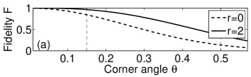
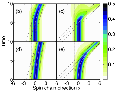
Figure 2: (a) Fidelity as a function of corner angle $\theta$, for two values of $r$: $r=0$ (discontinuous corner, solid line) and $r=2$ (smooth corner, dashed line). Fidelity decreases with increasing angle $\theta$ in accordance with conventional optical bend-loss. Four examples of magnon propagation are shown: (b) $r=0$, $\theta=0.15$ (fidelity 0.769), (c) $r=0$, $\theta=0.5$ (fidelity 0.106), (d) $r=2$, $\theta=0.15$, (fidelity 0.979) (e) $r=2$, $\theta=0.5$ (fidelity 0.401). In all cases, $t_{\rm f}=10$.

To study the effectiveness of the channel, we examine the spin-guide fidelity. The fidelity is given by the overlap between the initial wave function $\psi(x,t=0)$, and the excitation at the final time $t_{\rm f}$ (shifted back to the original location, $\psi^{*}[x+x_{0}(t_{f}),t=t_{\rm f}]$):

$$F=\left|\int_{-\infty}^{\infty}\psi(x,t=0)\psi^{*}[x+x_{0}(t_{\rm f}),t=t_{\rm f}]dx\right|^{2},$$ (4)

and $0\leq F\leq 1$.

An important concept with optical fibres is bend-loss, i.e. the extent to which an optical fibre can be bent before the mode ceases to be guided, and is therefore lost. The equivalent case is accelerating the magnon by investigating a single spin-guide with a ‘corner’. The centre of the spin-guide is given by

$$x_{0}(t)=\sqrt{r+\tan^{2}\theta(t-t_{\rm f}/2)^{2}}+\tan\theta(t-t_{\rm f}/2)$$ (5)

where $r$ indicates the sharpness of the corner, $\theta$ is the angle through which the spin-guide changes direction, and $t_{\rm f}$ is the final time. The excitation is initially centered at position $x_{0}(0)$, with momentum $k=\left.\partial x_{0}(t)/\partial t\right|_{t=0}$.

Fig. 2(a) utilises Eq. (5) to show how the fidelity decreases with increasing angle through which the spin-guide moves $\theta$. Two lines are shown: $r=0$ (discontinuous corner) always has lower fidelity than $r=2$ (smooth corner). As the corner is made more abrupt the fidelity decreases, in accordance with our intuition from optical bend-loss results. The evolution with different examples of $r$ and $\theta$ is shown in Fig. 2(b)-(d).

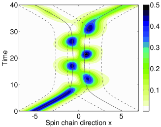
Figure 3: Magnon evolution through a spin-splitter with parallel component. Oscillatory behavior of the excitation between the spin-guides is observed. Here, $r=0.5$, $d=1.2$, $m=0.3$.

To complete the connection between spin-guides and waveguides, we turn our attention to two-port devices, i.e. we show how to create a ‘spin-splitter’ by analogy with beamsplitters. We firstly examine a spin-splitter with a parallel component, see Fig. 3. The centre of the potentials of the left and right spin-guides are given by the piecewise continuous function

$$x_{\rm right}(t) = -x_{\rm left}(t)=\left\{\begin{array}[]{ll}f(x,t)&t<t_{\rm f}/2\\ f(x,t_{\rm f}-t)&t\geq t_{\rm f}/2\end{array}\right.,$$ (8)

$$f(x,t) = \sqrt{r+\left(4mt+d-x_{\rm l}\right)^{2}/16}-mt+(d+x_{\rm l})/4,$$

where $m$ is the slope and $d$ is the separation between the parallel components of the spin-guide. The position of the excitation is initially in the left spin-guide, i.e. $\psi(x=x_{\rm left}(0),t=0)$, and the initial momentum is the slope of the left spin-guide at time $t=0$, that is $k=\left.\partial x_{\rm left}(t)/\partial t\right|_{t=0}$. In Fig. 3 the solid lines show $x_{\rm left}$ and $x_{\rm right}$, and the dashed lines show $x_{\rm left}\pm 2$ and $x_{\rm right}\pm 2$, which can be intuitively thought of as the ‘edge’ of the spin-guides. The excitation, after initially starting in the left spin-guide, oscillates between spin-guides, before leaving primarily through the right spin-guide. As expected, the length of the parallel section compared to the oscillation frequency controls the final output distribution. This behavior is important to note, as it corresponds to the small angle limit of the spin-splitter in the next section.

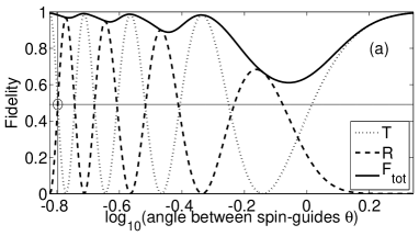
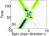
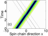
Figure 4: (a) Fidelity, and reflection and transmission coefficients for an X-junction spin-splitter as a function of spin-guide angle. The excitation is initialized in the left-to-right spin-guide and then evolved for time $t_{\rm f}=x_{l}/\tan(\theta/2)$ ($x_{l}=10$ fixed). The reflection and transmission coefficients show oscillations as expected from Landau-Zener theory. The spin-splitting fidelity is less than unity due to non-adiabaticity, although it asymptotes to one in both the small and large angle limits. (b) A 50/50 spin-splitter with $\theta=10^{-0.7976}$ (corresponding to $R\approx T\approx 0.491$, $F_{\rm tot}\approx 0.982$, indicated by a circle at the intersection of a horizontal and a vertical line). (c) A non-adiabatic crossing with $\theta=10^{2.2}$. Note the different time-scales in (b) and (c).

Coupling between spin-guides is the equivalent of evanescent tunneling between optical waveguides. Consider two parallel spin-guides, separated by distance $d$, with an initial excitation which has zero momentum, $k=0$. The oscillation frequency into and out of the left waveguide is found by expressing the evolution as a two-state problem and defining an effective Hamiltonian in the basis $\{\psi_{\rm left}(x,t),\psi^{\prime}_{\rm right}(x,t),\ldots\}$, where, $\psi^{\prime}_{\rm right}(x,t)$ is determined by Gram-Schmidt orthonormalization relative to $\psi_{\rm left}(x,t)$ and $\psi_{\rm right}(x,t)$ which are given by Eq. (3). The resulting oscillation frequency is (given by the difference between the eigenvalues of the effective Hamiltonian),

$$\Omega(d)=\frac{{\rm csch}^{2}d[{\rm cosh}\,3d+4d\,{\rm sinh}\,d-(8d^{2}+1){\rm cosh}\,d]}{{\rm cosh}\,2d-2d^{2}-1}.$$ (9)

This function monotonically decreases from $\Omega(0)=16/15$ to $\Omega(d)\approx 4e^{-d}$ for large $d$.

A more practical form of spin-splitter than the style in Fig. 3 is an X-junction of spin-guides. Two straight spin-guides of length $2x_{\rm l}$ cross at an angle $\theta$, where $x_{\rm R\rightarrow L}(t)=-x_{\rm L\rightarrow R}(t)=x_{\rm l}/2-\tan(\theta/2)t$. The initial excitation is placed in the left-to-right spin-guide, such that $x_{0}(0)=x_{\rm L\rightarrow R}(0)$, with momentum $k_{\rm L\rightarrow R}=\tan(\theta/2)$.

The evolution for the X-junction is shown in Fig. 4, for time $t_{\rm f}=x_{l}/\tan(\theta/2)$. The relevant metrics for the spin-splitter are shown in Fig. 4(a) as a function of spin-guide angle. The reflection and transmission coefficients $R$ and $T$, as defined by Eq. (4), and the total fidelity is $F_{\rm tot}=R+T$. The behavior of $R$ and $T$ can be understood with regard to Landau-Zener theory Landau (1932); Zener (1932). When $\theta$ is large, the spin-splitter shows a non-adiabatic crossing, therefore the reflection (transmission) coefficient approaches zero (one) for large $\theta$, Fig. 4(c). Conversely, when $\theta$ is small, the spin-guides approach an almost parallel state. As such, the excitation behaves similarly to Fig. 3, where the excitation oscillates between spin-guides and therefore the fidelity depends strongly on $\theta$. In contrast to conventional Landau-Zener this is not the adiabatic regime as the spin-guides are forced to cross and the interaction time increases with decreasing angle so that oscillations are always observed.

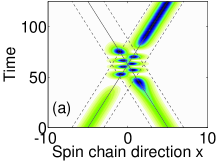
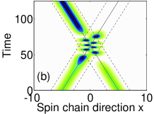
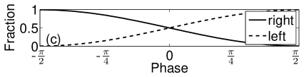
Figure 5: (a) [(b)] the evolution when the excitation is initialized as a superposition in both spin-guides, the phase between them is $\pi/2$ ($-\pi/2$). (c) The fraction of excitation in the left and right spin-guides as a function of the phase between the initial excitations.

An important spin-splitting ratio is 50/50 ($T=R$), and Fig. 4(a) shows many points where this ratio is approximately achieved, although with varying fidelity. An example, with $\theta=10^{-0.7976}$ is shown in Fig. 4(b), corresponding to the value of $\theta$ indicated by the circle intersecting the horizontal and vertical lines in Fig. 4(a), when $R\approx T\approx 0.491$ ($F_{\rm tot}\approx 0.982$). These are slightly less than 0.5 due to scattering into non-bound modes. By choosing a sufficiently small $\theta$, one can generate a 50/50 spin-splitter with a $T$ and $R$ arbitrarily close to 0.5.

Finally, using our spin-splitter we demonstrate the fundamental quantum mechanical characteristic of a beamsplitter: the interference of paths due to their relative phase. The wave function is initialized as $\psi(x,t=0)=\frac{1}{\sqrt{2}}[\psi_{\rm L\rightarrow R}(x,0)+$ $e^{i\alpha}\psi_{\rm R\rightarrow L}(x,0)]$. Fig. 5(a) shows the evolution when $\alpha=\pi/2$ , where the excitation emerges solely from the left-to-right spin-guide. Similarly, $\alpha=-\pi/2$ results in the excitation emerging from the right-to-left spin-guide [Fig. 5(b)]. The fraction in the left and right halves of the spin-chain as a function of the phase $\alpha$ is given in Fig. 5(c). This phase interference proves the quantum mechanical nature of the spin-splitter, thereby completing the analogy between optical waveguides and the behavior of spin-guides.

We have shown that a collective excitation within a linear spin-chain can be confined and manipulated using localized field modulation. Specifically, we see that the space-time behavior of this one-dimensional excitation mimics effects traditionally observed with linear optics experiments (in two spatial dimensions). Using suitably chosen field modulations in space and time, we can replicate optical guiding modes, beam-splitting and even phase interference. This technique provides a new conceptual framework and method for controlling spin excitations using field modulation over distances much greater than the spin-spin separation.

I Acknowledgments

M.I.M. acknowledges the support of the David Hay award. C.D.H. acknowledges support from the Australian Research Council Center of Excellence for Quantum Computation and Communication Technology (Project Number CE110001027). A.D.G. acknowledges the Australian Research Council for financial support (Project No. DP0880466).

References

- Bose (2007) S. Bose, Contemp. Phys. 48, 13 (2007).
- Copsey et al. (2003) D. Copsey, M. Oskin, F. Impens, T. Metodiev, A. Cross, F. T. Chong, I. L. Chuang, and J. Kubiatowicz, IEEE J. Sel. Top. Quantum Electron. 9, 1552 (2003).
- Heule et al. (2010) R. Heule, C. Bruder, D. Burgarth, and V.M. Stojanovic, Phys. Rev. A 82, 052333 (2010).
- Burgarth et al. (2009) D. Burgarth, S. Bose, C. Bruder, and V. Giovannetti, Phys. Rev. A 79, 060305 (2009).
- Kay (2011) A. Kay, Phys. Rev. A 84, 022337 (2011).
- Maloshtan and Kilin (2009) A. S. Maloshtan and S. Y. Kilin, Opt. and Spectros. 108, 406 (2009).
- Mogilevtsev et al. (2010) D. Mogilevtsev, A. Maloshtan, S. Kilin, L. E. Oliveira, and S. B. Cavalcanti, J. Phys. B 43, 095506 (2010).
- Christandl et al. (2004) M. Christandl, N. Datta, A. Ekert, and A. J. Landahl, Phys. Rev. Lett. 92, 187902 (2004).
- Ohshima et al. (2007) T. Ohshima, A. Ekert, D. K. L. Oi, D. Kaslizowski, and L. C. Kwek, arXiv:quant-ph/0702019 (2007).
- Zhou et al. (2008) L. Zhou, Z. R. Gong, Y. X. Liu, C. P. Sun, and F. Nori, Phys. Rev. Lett. 101, 100501 (2008).
- Liao et al. (2010) J. Q. Liao, Z. R. Gong, L. Zhou, Y. X. Liu, C. P. Sun, and F. Nori, Phys. Rev. A 81, 042304 (2010).
- Makin et al. (2009) M. I. Makin, J. H. Cole, C. D. Hill, A. D. Greentree, and L. C. L. Hollenberg, Phys. Rev. A 80, 043842 (2009).
- Kranendonk and Vleck (1958) J. V. Kranendonk and J. H. V. Vleck, Rev. Mod. Phys. 30, 1 (1958).
- Ladouceur and Love (1996) F. Ladouceur and J. D. Love, Silica-based buried channel waveguides and devices (London, Chapman and Hall, 1996).
- Osborne and Linden (2004) T. J. Osborne and N. Linden, Phys. Rev. A 69, 052315 (2004).
- Skinner et al. (2003) A. J. Skinner, M. E. Davenport, and B. E. Kane, Phys. Rev. Lett. 90, 087901 (2003).
- Taylor et al. (2005) J. M. Taylor, H. A. Engel, W. Dür, A. Yacoby, C. M. Marcus, P. Zoller, and M. D. Lukin, Nat. Phys. 1, 177 (2005).
- Pöschl and Teller (1933) G. Pöschl and E. Teller, Z. Phys. 83, 143 (1933).
- Rosen and Morse (1932) N. Rosen and P. M. Morse, Phys. Rev. 42, 210 (1932).
- Eckart (1930) C. Eckart, Phys. Rev. 35, 1303 (1930).
- Landau (1932) L. D. Landau, Phys. Z 2, 46 (1932).
- Zener (1932) C. Zener, Proc. R. Soc. London A 137, 696 (1932).