Algorithms for geodesics

Abstract

Algorithms for the computation of geodesics on an ellipsoid of revolution are given. These provide accurate, robust, and fast solutions to the direct and inverse geodesic problems and they allow differential and integral properties of geodesics to be computed.

1 Introduction

The shortest path between two points on the earth, customarily treated as an ellipsoid of revolution, is called a geodesic. Two geodesic problems are usually considered: the direct problem of finding the end point of a geodesic given its starting point, initial azimuth, and length; and the inverse problem of finding the shortest path between two given points. Referring to Fig. 1, it can be seen that each problem is equivalent to solving the geodesic triangle $N\!AB$ given two sides and their included angle (the azimuth at the first point, $\alpha_{1}$, in the case of the direct problem and the longitude difference, $\lambda_{12}$, in the case of the inverse problem). The framework for solving these problems was laid down by Legendre (1806), Oriani (1806, 1808, 1810), Bessel (1825), and Helmert (1880). Based on these works, Vincenty (1975a) devised algorithms for solving the geodesic problems suitable for early programmable desk calculators; these algorithms are in widespread use today. A good summary of Vincenty’s algorithms and the earlier work in the field is given by Rapp (1993, Chap. 1).

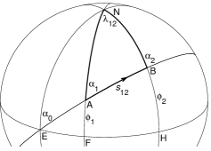
Figure 1: The ellipsoidal triangle $N\!AB$. $N$ is the north pole, $N\!AF$ and $N\!BH$ are meridians, and $AB$ is a geodesic of length $s_{12}$. The longitude of $B$ relative to $A$ is $\lambda_{12}$; the latitudes of $A$ and $B$ are $\phi_{1}$ and $\phi_{2}$. $EF\!H$ is the equator with $E$ also lying on the extension of the geodesic $AB$; and $\alpha_{0}$, $\alpha_{1}$, and $\alpha_{2}$ are the azimuths (in the forward direction) of the geodesic at $E$, $A$, and $B$.

The goal of this paper is to adapt the geodesic methods of Helmert (1880) and his predecessors to modern computers. The current work goes beyond Vincenty in three ways: (1) The accuracy is increased to match the standard precision of most computers. This is a relatively straightforward task of retaining sufficient terms in the series expansions and can be achieved at little computational cost. (2) A solution of the inverse problem is given which converges for all pairs of points. (Vincenty’s method fails to converge for nearly antipodal points.) (3) Differential and integral properties of the geodesics are computed. The differential properties allow the behavior of nearby geodesics to be determined, which enables the scales of geodesic projections to be computed without resorting to numerical differentiation; crucially, one of the differential quantities is also used in the solution of the inverse problem. The integral properties provide a method for finding the area of a geodesic polygon, extending the work of Danielsen (1989).

Section 2 reviews the classical solution of geodesic problem by means of the auxiliary sphere and provides expansions of the resulting integrals accurate to $O(f^{6})$ (where $f$ is the flattening of the ellipsoid). These expansions can be inserted into the solution for the direct geodesic problem presented by, for example, Rapp (1993) to provide accuracy to machine precision. Section 3 gives the differential properties of geodesics reviewing the results of Helmert (1880) for the reduced length and geodesic scale and give the key properties of these quantities and appropriate series expansions to allow them to be calculated accurately. Knowledge of the reduced length enables the solution of the inverse problem by Newton’s method which is described in Sect. 4. Newton’s method requires a good starting guess and, in the case of nearly antipodal points, this is provided by an approximate solution of the inverse problem by Helmert (1880), as given in Sect. 5. The computation of area between a geodesic and the equator is formulated in Sect. 6, extending the work of Danielsen (1989). Some details of the implementation and present accuracy and timing data are discussed in Sect. 7. As an illustration of the use of these algorithms, Sect. 8 gives an ellipsoidal gnomonic projection in which geodesics are very nearly straight. This provides a convenient way of solving several geodesic problems.

For the purposes of this paper, it is useful to generalize the definition of a geodesic. The geodesic curvature, $\kappa$, of an arbitrary curve at a point $P$ on a surface is defined as the curvature of the projection of the curve onto a plane tangent to the surface at $P$. All shortest paths on a surface are straight, defined as $\kappa=0$ at every point on the path. In the rest of this paper, I use straightness as the defining property of geodesics; this allows geodesic lines to be extended indefinitely (beyond the point at which they cease to be shortest paths).

Several of the results reported here appeared earlier in a technical report, Karney (2011).

2 Basic Equations and Direct Problem

I consider an ellipsoid of revolution with equatorial radius $a$, and polar semi-axis $b$, flattening $f$, third flattening $n$, eccentricity $e$, and second eccentricity $e^{\prime}$ given by

$$f =(a-b)/a=1-\sqrt{1-e^{2}},$$ (1)

$$n =(a-b)/(a+b)=f/(2-f),$$ (2)

$$e^{2} =(a^{2}-b^{2})/a^{2}=f(2-f),$$ (3)

$$e^{\prime 2} =(a^{2}-b^{2})/b^{2}=e^{2}/(1-e^{2}).$$ (4)

As a consequence of the rotational symmetry of the ellipsoid, geodesics obey a relation found by Clairaut (1735), namely

$$\sin\alpha_{0}=\sin\alpha_{1}\cos\beta_{1}=\sin\alpha_{2}\cos\beta_{2},$$ (5)

where $\beta$ is the reduced latitude (sometimes called the parametric latitude), given by

$$\tan\beta=(1-f)\tan\phi.$$ (6)

The geodesic problems are most easily solved by using an auxiliary sphere which allows an exact correspondence to be made between a geodesic and a great circle on a sphere. On the sphere, the latitude $\phi$ is replaced by the reduced latitude $\beta$, and azimuths $\alpha$ are preserved. From Fig. 2, it is clear that Clairaut’s equation, $\sin\alpha_{0}=\sin\alpha\cos\beta$, is just the sine rule applied to the sides $N\!E$ and $N\!P$ of the triangle $N\!EP$ and their opposite angles. The third side, the spherical arc length $\sigma$, and its opposite angle, the spherical longitude $\omega$, are related to the equivalent quantities on the ellipsoid, the distance $s$ and longitude $\lambda$, by (Rapp, 1993, Eqs. (1.28) and (1.170))

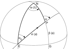
Figure 2: The elementary ellipsoidal triangle $N\!EP$ mapped to the auxiliary sphere. $N\!E$ and $N\!PG$ are meridians; $EG$ is the equator; and $EP$ is the great circle (i.e., the geodesic). The corresponding ellipsoidal variables are shown in parentheses. Here $P$ represents an arbitrary point on the geodesic $EAB$ in Fig. 1.

$$\frac{s}{b} =\int_{0}^{\sigma}\sqrt{1+k^{2}\sin^{2}\sigma^{\prime}}\,\mathrm{d}\sigma^{\prime}=I_{1}(\sigma),$$ (7)

$$\lambda =\omega-f\sin\alpha_{0}\int_{0}^{\sigma}\frac{2-f}{1+(1-f)\sqrt{1+k^{2}\sin^{2}\sigma^{\prime}}}\,\mathrm{d}\sigma^{\prime}$$

$$=\omega-f\sin\alpha_{0}\,I_{3}(\sigma),$$ (8)

where

$$k=e^{\prime}\cos\alpha_{0}.$$ (9)

See also Eqs. (5.4.9) and (5.8.8) of Helmert (1880). The origin for $s$, $\sigma$, $\lambda$, and $\omega$ is the point $E$, at which the geodesic crosses the equator in the northward direction, with azimuth $\alpha_{0}$. The point $P$ can stand for either end of the geodesic $AB$ in Fig. 1, with the quantities $\beta$, $\alpha$, $\sigma$, $\omega$, $s$, and $\lambda$ acquiring a subscript $1$ or $2$. I also define $s_{12}=s_{2}-s_{1}$ as the length of $AB$, with $\lambda_{12}$, $\sigma_{12}$, and $\omega_{12}$ defined similarly. (In this paper, $\alpha_{2}$ is the forward azimuth at $B$. Several authors use the back azimuth instead; this is given by $\alpha_{2}\pm\pi$.)

Because Eqs. (7) and (8) depend on $\alpha_{0}$, the mapping between the ellipsoid and the auxiliary sphere is not a global mapping of one surface to another; rather the auxiliary sphere should merely be regarded as a useful mathematical technique for solving geodesic problems. Similarly, because the origin for $\lambda$ depends on the geodesic, only longitude differences, e.g., $\lambda_{12}$, should be used in converting between longitudes relative to the prime meridian and $\lambda$.

In solving the spherical trigonometrical problems, the following equations relating the sides and angles of $N\!EP$ are useful,

$$\alpha_{0} =\mathop{\mathrm{ph}}\nolimits(\left|\cos\alpha+i\sin\alpha\sin\beta\right|+i\sin\alpha\cos\beta),$$ (10)

$$\sigma =\mathop{\mathrm{ph}}\nolimits(\cos\alpha\cos\beta+i\sin\beta),$$ (11)

$$\omega =\mathop{\mathrm{ph}}\nolimits(\cos\sigma+i\sin\alpha_{0}\sin\sigma),$$ (12)

$$\beta =\mathop{\mathrm{ph}}\nolimits(\left|\cos\alpha_{0}\cos\sigma+i\sin\alpha_{0}\right|+i\cos\alpha_{0}\sin\sigma),$$ (13)

$$\alpha =\mathop{\mathrm{ph}}\nolimits(\cos\alpha_{0}\cos\sigma+i\sin\alpha_{0}),$$ (14)

where $i=\sqrt{-1}$ and $\mathop{\mathrm{ph}}\nolimits(x+iy)$ is the phase of a complex number (Olver et al., 2010, §http://dlmf.nist.gov/1.9.i), typically given by the library function $\mathop{\mathrm{atan2}}\nolimits(y,x)$. Equation (10) merely recasts Eq. (5) in a form that allows it to be evaluated accurately when $\alpha_{0}$ is close to $\frac{1}{2}\pi$. The other relations are obtained by applying Napier’s rules of circular parts to $N\!EP$.

The distance integral, Eq. (7), can be expanded in a Fourier series

$$I_{1}(\sigma)=A_{1}\Bigl{(}\sigma+\sum_{l=1}^{\infty}C_{1l}\sin 2l\sigma\Bigr{)},$$ (15)

with the coefficients determined by expanding the integral in a Taylor series. It is advantageous to follow Bessel (1825, §5) and Helmert (1880, Eq. (5.5.1)) and use $\epsilon$, defined by

$$\epsilon=\frac{\sqrt{1+k^{2}}-1}{\sqrt{1+k^{2}}+1}\quad\text{or}\quad k=\frac{2\sqrt{\epsilon}}{1-\epsilon},$$ (16)

as the expansion parameter. This leads to expansions with half as many terms as the corresponding ones in $k^{2}$. The expansion can be conveniently carried out to arbitrary order by a computer algebra system such as Maxima (2009) which yields

$$A_{1} =(1-\epsilon)^{-1}\bigl{(}1+{\textstyle\frac{1}{4}}\epsilon^{2}+{\textstyle\frac{1}{64}}\epsilon^{4}+{\textstyle\frac{1}{256}}\epsilon^{6}+\cdots\bigr{)},$$ (17)

$$C_{11} =-{\textstyle\frac{1}{2}}\epsilon+{\textstyle\frac{3}{16}}\epsilon^{3}-{\textstyle\frac{1}{32}}\epsilon^{5}+\cdots,$$

$$C_{12} =-{\textstyle\frac{1}{16}}\epsilon^{2}+{\textstyle\frac{1}{32}}\epsilon^{4}-{\textstyle\frac{9}{2048}}\epsilon^{6}+\cdots,$$

$$C_{13} =-{\textstyle\frac{1}{48}}\epsilon^{3}+{\textstyle\frac{3}{256}}\epsilon^{5}+\cdots,$$

$$C_{14} =-{\textstyle\frac{5}{512}}\epsilon^{4}+{\textstyle\frac{3}{512}}\epsilon^{6}+\cdots,$$

$$C_{15} =-{\textstyle\frac{7}{1280}}\epsilon^{5}+\cdots,$$

$$C_{16} =-{\textstyle\frac{7}{2048}}\epsilon^{6}+\cdots.$$ (18)

This extends Eq. (5.5.7) of Helmert (1880) to higher order. These coefficients may be inserted into Eq. (1.40) of Rapp (1993) using

$$\mathcal{B}_{j}=\begin{cases}A_{1},&\text{for $j=0$},\\ 2A_{1}C_{1l},&\text{for $j=2l$, with $l>0$},\end{cases}$$ (19)

where here, and subsequently in Eqs. (22) and (26), a script letter, e.g., $\mathcal{B}$, is used to stand for Rapp’s coefficients.

In the course of solving the direct geodesic problem (where $s_{12}$ is given), it is necessary to determine $\sigma$ given $s$. Vincenty solves for $\sigma$ iteratively. However, it is simpler to follow Helmert (1880, §5.6) and substitute $s=bA_{1}\tau$ into Eqs. (7) and (15), to obtain $\tau=\sigma+\sum_{l}C_{1l}\sin 2l\sigma$; this may be inverted, for example, using Lagrange reversion, to give

$$\sigma=\tau+\sum_{l=1}^{\infty}C^{\prime}_{1l}\sin 2l\tau,$$ (20)

where

$$C^{\prime}_{11} ={\textstyle\frac{1}{2}}\epsilon-{\textstyle\frac{9}{32}}\epsilon^{3}+{\textstyle\frac{205}{1536}}\epsilon^{5}+\cdots,$$

$$C^{\prime}_{12} ={\textstyle\frac{5}{16}}\epsilon^{2}-{\textstyle\frac{37}{96}}\epsilon^{4}+{\textstyle\frac{1335}{4096}}\epsilon^{6}+\cdots,$$

$$C^{\prime}_{13} ={\textstyle\frac{29}{96}}\epsilon^{3}-{\textstyle\frac{75}{128}}\epsilon^{5}+\cdots,$$

$$C^{\prime}_{14} ={\textstyle\frac{539}{1536}}\epsilon^{4}-{\textstyle\frac{2391}{2560}}\epsilon^{6}+\cdots,$$

$$C^{\prime}_{15} ={\textstyle\frac{3467}{7680}}\epsilon^{5}+\cdots,$$

$$C^{\prime}_{16} ={\textstyle\frac{38081}{61440}}\epsilon^{6}+\cdots.$$ (21)

This extends Eq. (5.6.8) of Helmert (1880) to higher order. These coefficients may be used in Eq. (1.142) of Rapp (1993) using

$$\mathcal{D}_{j}=2C^{\prime}_{1l},\quad\text{for $j=2l$, with $l>0$}.$$ (22)

Similarly, the integral appearing in the longitude equation, Eq. (8), can be written as a Fourier series

$$I_{3}(\sigma)=A_{3}\Bigl{(}\sigma+\sum_{l=1}^{\infty}C_{3l}\sin 2l\sigma\Bigr{)}.$$ (23)

Following Helmert (1880), I expand jointly in $n$ and $\epsilon$, both of which are $O(f)$, to give

$$A_{3} =1-\bigl{(}{\textstyle\frac{1}{2}}-{\textstyle\frac{1}{2}}n\bigr{)}\epsilon-\bigl{(}{\textstyle\frac{1}{4}}+{\textstyle\frac{1}{8}}n-{\textstyle\frac{3}{8}}n^{2}\bigr{)}\epsilon^{2}$$

$$\qquad{}-\bigl{(}{\textstyle\frac{1}{16}}+{\textstyle\frac{3}{16}}n+{\textstyle\frac{1}{16}}n^{2}\bigr{)}\epsilon^{3}-\bigl{(}{\textstyle\frac{3}{64}}+{\textstyle\frac{1}{32}}n\bigr{)}\epsilon^{4}$$

$$\qquad{}-{\textstyle\frac{3}{128}}\epsilon^{5}+\cdots,$$ (24)

$$C_{31} =\bigl{(}{\textstyle\frac{1}{4}}-{\textstyle\frac{1}{4}}n\bigr{)}\epsilon+\bigl{(}{\textstyle\frac{1}{8}}-{\textstyle\frac{1}{8}}n^{2}\bigr{)}\epsilon^{2}+\bigl{(}{\textstyle\frac{3}{64}}+{\textstyle\frac{3}{64}}n-{\textstyle\frac{1}{64}}n^{2}\bigr{)}\epsilon^{3}$$

$$\quad{}+\bigl{(}{\textstyle\frac{5}{128}}+{\textstyle\frac{1}{64}}n\bigr{)}\epsilon^{4}+{\textstyle\frac{3}{128}}\epsilon^{5}+\cdots,$$

$$C_{32} =\bigl{(}{\textstyle\frac{1}{16}}-{\textstyle\frac{3}{32}}n+{\textstyle\frac{1}{32}}n^{2}\bigr{)}\epsilon^{2}+\bigl{(}{\textstyle\frac{3}{64}}-{\textstyle\frac{1}{32}}n-{\textstyle\frac{3}{64}}n^{2}\bigr{)}\epsilon^{3}$$

$$\quad{}+\bigl{(}{\textstyle\frac{3}{128}}+{\textstyle\frac{1}{128}}n\bigr{)}\epsilon^{4}+{\textstyle\frac{5}{256}}\epsilon^{5}+\cdots,$$

$$C_{33} =\bigl{(}{\textstyle\frac{5}{192}}-{\textstyle\frac{3}{64}}n+{\textstyle\frac{5}{192}}n^{2}\bigr{)}\epsilon^{3}+\bigl{(}{\textstyle\frac{3}{128}}-{\textstyle\frac{5}{192}}n\bigr{)}\epsilon^{4}$$

$$\quad{}+{\textstyle\frac{7}{512}}\epsilon^{5}+\cdots,$$

$$C_{34} =\bigl{(}{\textstyle\frac{7}{512}}-{\textstyle\frac{7}{256}}n\bigr{)}\epsilon^{4}+{\textstyle\frac{7}{512}}\epsilon^{5}+\cdots,$$

$$C_{35} ={\textstyle\frac{21}{2560}}\epsilon^{5}+\cdots.$$ (25)

This extends Eq. (5.8.14) of Helmert (1880) to higher order. These coefficients may be inserted into Eq. (1.56) of Rapp (1993) using

$$\mathcal{A}_{j}=\begin{cases}A_{3},&\text{for $j=0$},\\ 2A_{3}C_{3l},&\text{for $j=2l$, with $l>0$}.\end{cases}$$ (26)

Table 1: The parameters for the WGS84 ellipsoid used in the examples. The column labeled “Eq.” lists the equations used to compute the corresponding quantities.

Qty.	Value	Eq.
$a$	$6\,378\,137\,\mathrm{m}$	given
$f$	$1/298.257\,223\,563$	given
$b$	$6\,356\,752.314\,245\,\mathrm{m}$	(1)
$c$	$6\,371\,007.180\,918\,\mathrm{m}$	(60)
$n$	$0.001\,679\,220\,386\,383\,70$	(2)
$e^{2}$	$0.006\,694\,379\,990\,141\,32$	(3)
$e^{\prime 2}$	$0.006\,739\,496\,742\,276\,43$	(4)

Table 2: A sample direct calculation specified by $\phi_{1}=40^{\circ}$, $\alpha_{1}=30^{\circ}$, and $s_{12}=10\,000\,\mathrm{km}$. For equatorial geodesics ($\phi_{1}=0$ and $\alpha_{1}=\frac{1}{2}\pi$), Eq. (11) is indeterminate; in this case, take $\sigma_{1}=0$.

Qty.	Value	Eq.
$\phi_{1}$	$40^{\circ}$	given
$\alpha_{1}$	$30^{\circ}$	given
$s_{12}$	$10\,000\,000\,\mathrm{m}$	given
Solve triangle $N\!EA$
$\beta_{1}$	$39.905\,277\,146\,01^{\circ}$	(6)
$\alpha_{0}$	$22.553\,940\,202\,62^{\circ}$	(10)
$\sigma_{1}$	$43.999\,153\,645\,00^{\circ}$	(11)
$\omega_{1}$	$20.323\,718\,278\,37^{\circ}$	(12)
Determine $\sigma_{2}$
$k^{2}$	$0.005\,748\,029\,628\,57$	(9)
$\epsilon$	$0.001\,432\,892\,204\,16$	(16)
$A_{1}$	$1.001\,435\,462\,362\,07$	(17)
$I_{1}(\sigma_{1})$	$0.768\,315\,388\,864\,12$	(15)
$s_{1}$	$\hphantom{0}4\,883\,990.626\,232\,\mathrm{m}$	(7)
$s_{2}$	$14\,883\,990.626\,232\,\mathrm{m}$	$s_{1}+s_{12}$
$\tau_{2}$	$133.962\,660\,502\,08^{\circ}$	$s_{2}/(bA_{1})$
$\sigma_{2}$	$133.921\,640\,830\,38^{\circ}$	(20)
Solve triangle $N\!EB$
$\alpha_{2}$	$149.090\,169\,318\,07^{\circ}$	(14)
$\beta_{2}$	$\hphantom{0}41.697\,718\,092\,50^{\circ}$	(13)
$\omega_{2}$	$158.284\,121\,471\,12^{\circ}$	(12)
Determine $\lambda_{12}$
$A_{3}$	$0.999\,284\,243\,06$	(24)
$I_{3}(\sigma_{1})$	$0.767\,737\,860\,69$	(23)
$I_{3}(\sigma_{2})$	$2.335\,343\,221\,70$	(23)
$\lambda_{1}$	$\hphantom{0}20.267\,150\,380\,16^{\circ}$	(8)
$\lambda_{2}$	$158.112\,050\,423\,93^{\circ}$	(8)
$\lambda_{12}$	$137.844\,900\,043\,77^{\circ}$	$\lambda_{2}-\lambda_{1}$
Solution
$\phi_{2}$	$\hphantom{0}41.793\,310\,205\,06^{\circ}$	(6)
$\lambda_{12}$	$137.844\,900\,043\,77^{\circ}$
$\alpha_{2}$	$149.090\,169\,318\,07^{\circ}$

The equations given in this section allow the direct geodesic problem to be solved. Given $\phi_{1}$ (and hence $\beta_{1}$) and $\alpha_{1}$ solve the spherical triangle $N\!EA$ to give $\alpha_{0}$, $\sigma_{1}$, and $\omega_{1}$ using Eqs. (10), (11), and (12). Find $s_{1}$ and $\lambda_{1}$ from Eqs. (7) and (8) together with Eqs. (15) and (23). (Recall that the origin for $\lambda$ is $E$ in Fig. 1.) Determine $s_{2}=s_{1}+s_{12}$ and hence $\sigma_{2}$ using Eq. (20). Now solve the spherical triangle $N\!EB$ to give $\alpha_{2}$, $\beta_{2}$ (and hence $\phi_{2}$), and $\omega_{2}$, using Eqs. (14), (13), and (12). Finally, determine $\lambda_{2}$ (and $\lambda_{12}$) from Eqs. (8) and (23). A numerical example of the solution of the direct problem is given in Table 2 using the parameters of Table 1.

3 Differential Quantities

Before turning to the inverse problem, I present Gauss’ solution for the differential behavior of geodesics. One differential quantity, the reduced length $m_{12}$, is needed in the solution of the inverse problem by Newton’s method (Sect. 4) and an expression for this quantity is given at the end of this section. However, because this and other differential quantities aid in the solution of many geodesic problems, I also discuss their derivation and present some of their properties.

Consider a reference geodesic parametrized by distance $s$ and a nearby geodesic separated from the reference by infinitesimal distance $t(s)$. Gauss (1828) showed that $t(s)$ satisfies the differential equation

$$\frac{\mathrm{d}^{2}t(s)}{\mathrm{d}s^{2}}+K(s)\,t(s)=0,$$ (27)

where $K(s)$ is the Gaussian curvature of the surface. As a second order, linear, homogeneous differential equation, its solution can be written as

$$t(s)=At_{A}(s)+Bt_{B}(s),$$

where $A$ and $B$ are (infinitesimal) constants and $t_{A}$ and $t_{B}$ are independent solutions. When considering the geodesic segment spanning $s_{1}\leq s\leq s_{2}$, it is convenient to specify

$$t_{A}(s_{1}) =0,\quad\left.\frac{\mathrm{d}t_{A}(s)}{\mathrm{d}s}\right|_{s=s_{1}}=1,$$

$$t_{B}(s_{1}) =1,\quad\left.\frac{\mathrm{d}t_{B}(s)}{\mathrm{d}s}\right|_{s=s_{1}}=0,$$

and to write

$$m_{12}=t_{A}(s_{2}),\quad M_{12}=t_{B}(s_{2}).$$

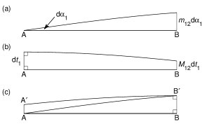
Figure 3: The definitions of $m_{12}$ and $M_{12}$ are illustrated in (a) and (b). A geometric proof of Eq. (29) is shown in (c); here $AB$ and $A^{\prime}B^{\prime}$ are parallel at $B$ and $B^{\prime}$, $BAB^{\prime}=\mathrm{d}\alpha_{1}$, $BB^{\prime}=m_{12}\,\mathrm{d}\alpha_{1}$, $AA^{\prime}=M_{21}m_{12}\,\mathrm{d}\alpha_{1}$, and finally $AB^{\prime}A^{\prime}=M_{21}\,\mathrm{d}\alpha_{1}$, from which Eq. (29) follows.

The quantity $m_{12}$ is the reduced length of the geodesic (Christoffel, 1868). Consider two geodesics which cross at $s=s_{1}$ at a small angle $\mathrm{d}\alpha_{1}$, Fig 3(a); at $s=s_{2}$, they will be separated by a distance $m_{12}\,\mathrm{d}\alpha_{1}$. Similarly I call $M_{12}$ the geodesic scale. Consider two geodesics which are parallel at $s=s_{1}$ and separated by a small distance $\mathrm{d}t_{1}$, Fig 3(b); at $s=s_{2}$, they will be separated by a distance $M_{12}\,\mathrm{d}t_{1}$.

Several relations between $m_{12}$ and $M_{12}$ follow from the defining equation, Eq. (27). The reduced length obeys a reciprocity relation (Christoffel, 1868, §9), $m_{21}+m_{12}=0$; the Wronskian is given by

$$W(M_{12},m_{12})(s_{2})=M_{12}\frac{\mathrm{d}m_{12}}{\mathrm{d}s_{2}}-m_{12}\frac{\mathrm{d}M_{12}}{\mathrm{d}s_{2}}=1;$$ (28)

and the derivatives are

$$\frac{\mathrm{d}m_{12}}{\mathrm{d}s_{2}} =M_{21},$$ (29)

$$\frac{\mathrm{d}M_{12}}{\mathrm{d}s_{2}} =-\frac{1-M_{12}M_{21}}{m_{12}}.$$ (30)

The constancy of the Wronskian follows by noting that its derivative with respect to $s_{2}$ vanishes; its value is found by evaluating it at $s_{2}=s_{1}$. A geometric proof of Eq. (29) is given in Fig 3(c) and Eq. (30) then follows from Eq. (28). With knowledge of the derivatives, addition rules for $m_{12}$ and $M_{12}$ are easily found,

$$m_{13} =m_{12}M_{23}+m_{23}M_{21},$$ (31)

$$M_{13} =M_{12}M_{23}-(1-M_{12}M_{21})\frac{m_{23}}{m_{12}},$$ (32)

$$M_{31} =M_{32}M_{21}-(1-M_{23}M_{32})\frac{m_{12}}{m_{23}},$$ (33)

where points 1, 2, and 3 all lie on the same geodesic.

Geodesics allow concepts from plane geometry to be generalized to apply to a curved surface. In particular, a geodesic circle may be defined as the curve which is a constant geodesic distance from a fixed point. Similarly, a geodesic parallel to a reference curve is the curve which is a constant geodesic distance from that curve. (Thus a circle is a special case of a parallel obtained in the limit when the reference curve degenerates to a point.) Parallels occur naturally when considering, for example, the “12-mile limit” for territorial waters which is the boundary of points lying within 12 nautical miles of a coastal state.

The geodesic curvature of a parallel can be expressed in terms of $m_{12}$ and $M_{12}$. Let point 1 be an arbitrary point on the reference curve with geodesic curvature $\kappa_{1}$. Point 2 is the corresponding point on the parallel, a fixed distance $s_{12}$ away. The geodesic curvature of the parallel at that point is found from Eqs. (29) and (30),

$$\kappa_{2}=\frac{M_{21}\kappa_{1}-(1-M_{12}M_{21})/m_{12}}{m_{12}\kappa_{1}+M_{12}}.$$ (34)

The curvature of a circle is given by the limit $\kappa_{1}\rightarrow\infty$,

$$\kappa_{2}=M_{21}/m_{12}.$$ (35)

If the reference curve is a geodesic ($\kappa_{1}\rightarrow 0$), then the curvature of its parallel is

$$\kappa_{2}=-(1-M_{12}M_{21})/(M_{12}m_{12}).$$ (36)

If the reference curve is indented, then the parallel intersects itself at a sufficiently large distance from the reference curve. This begins to happen when $\kappa_{2}\rightarrow\infty$ in Eq. (34).

The results above apply to general surfaces. For a geodesic on an ellipsoid of revolution, the Gaussian curvature of the surface is given by

$$K=\frac{(1-e^{2}\sin^{2}\phi)^{2}}{b^{2}}=\frac{1}{b^{2}(1+k^{2}\sin^{2}\sigma)^{2}}.$$ (37)

Helmert (1880, Eq. (6.5.1)) solves Eq. (27) in this case to give

$$m_{12}/b =\sqrt{\vphantom{\sin^{2}k^{2}}\smash{1+k^{2}\sin^{2}\sigma_{2}}}\,\cos\sigma_{1}\sin\sigma_{2}$$

$$\quad-\sqrt{\vphantom{\sin^{2}k^{2}}\smash{1+k^{2}\sin^{2}\sigma_{1}}}\,\sin\sigma_{1}\cos\sigma_{2}$$

$$\quad-\cos\sigma_{1}\cos\sigma_{2}\bigl{(}J(\sigma_{2})-J(\sigma_{1})\bigr{)},$$ (38)

$$M_{12} =\cos\sigma_{1}\cos\sigma_{2}+\frac{\sqrt{1+k^{2}\sin^{2}\sigma_{2}}}{\sqrt{1+k^{2}\sin^{2}\sigma_{1}}}\sin\sigma_{1}\sin\sigma_{2}$$

$$\quad-\frac{\sin\sigma_{1}\cos\sigma_{2}\bigl{(}J(\sigma_{2})-J(\sigma_{1})\bigr{)}}{\sqrt{1+k^{2}\sin^{2}\sigma_{1}}},$$ (39)

where

$$J(\sigma) =\int_{0}^{\sigma}\frac{k^{2}\sin^{2}\sigma^{\prime}}{\sqrt{1+k^{2}\sin^{2}\sigma^{\prime}}}\,\mathrm{d}\sigma^{\prime}$$

$$=\frac{s}{b}-\int_{0}^{\sigma}\frac{1}{\sqrt{1+k^{2}\sin^{2}\sigma^{\prime}}}\,\mathrm{d}\sigma^{\prime}$$

$$=I_{1}(\sigma)-I_{2}(\sigma).$$ (40)

Equation (39) may be obtained from Eq. (6.9.7) of Helmert (1880), which gives $\mathrm{d}m_{12}/\mathrm{d}s_{2}$; $M_{12}$ may then be found from Eq. (29) with an interchange of indices. In the spherical limit, $f\rightarrow 0$, Eqs. (38) and (39) reduce to

$$m_{12} =a\sin\sigma_{12}=a\sin(s_{12}/a),$$

$$M_{12} =\cos\sigma_{12}=\cos(s_{12}/a).$$

The integral $I_{2}(\sigma)$ in Eq. (3) may be expanded in a Fourier series in similar fashion to $I_{1}(\sigma)$, Eq. (15),

$$I_{2}(\sigma)=A_{2}\Bigl{(}\sigma+\sum_{l=1}^{\infty}C_{2l}\sin 2l\sigma\Bigr{)},$$ (41)

where

$$A_{2} =(1-\epsilon)\bigl{(}1+{\textstyle\frac{1}{4}}\epsilon^{2}+{\textstyle\frac{9}{64}}\epsilon^{4}+{\textstyle\frac{25}{256}}\epsilon^{6}+\cdots\bigr{)},$$ (42)

$$C_{21} ={\textstyle\frac{1}{2}}\epsilon+{\textstyle\frac{1}{16}}\epsilon^{3}+{\textstyle\frac{1}{32}}\epsilon^{5}+\cdots,$$

$$C_{22} ={\textstyle\frac{3}{16}}\epsilon^{2}+{\textstyle\frac{1}{32}}\epsilon^{4}+{\textstyle\frac{35}{2048}}\epsilon^{6}+\cdots,$$

$$C_{23} ={\textstyle\frac{5}{48}}\epsilon^{3}+{\textstyle\frac{5}{256}}\epsilon^{5}+\cdots,$$

$$C_{24} ={\textstyle\frac{35}{512}}\epsilon^{4}+{\textstyle\frac{7}{512}}\epsilon^{6}+\cdots,$$

$$C_{25} ={\textstyle\frac{63}{1280}}\epsilon^{5}+\cdots,$$

$$C_{26} ={\textstyle\frac{77}{2048}}\epsilon^{6}.$$ (43)

4 Inverse Problem

The inverse problem is intrinsically more complicated than the direct problem because the given included angle, $\lambda_{12}$ in Fig. 1, is related to the corresponding angle on the auxiliary sphere $\omega_{12}$ via an unknown equatorial azimuth $\alpha_{0}$. Thus, the inverse problem inevitably becomes a root-finding exercise.

I tackle this problem as follows. Assume that $\alpha_{1}$ is known. Solve the hybrid geodesic problem: given $\phi_{1}$, $\phi_{2}$, and $\alpha_{1}$, find $\lambda_{12}$ corresponding to the first intersection of the geodesic with the circle of latitude $\phi_{2}$. The resulting $\lambda_{12}$ differs, in general, from the given $\lambda_{12}$; so adjust $\alpha_{1}$ using Newton’s method until the correct $\lambda_{12}$ is obtained.

I begin by putting the points in a canonical configuration,

$$\phi_{1}\leq 0,\quad\phi_{1}\leq\phi_{2}\leq-\phi_{1},\quad 0\leq\lambda_{12}\leq\pi.$$ (44)

This may be accomplished swapping the end points and the signs of the coordinates if necessary, and the solution may similarly be transformed to apply to the original points. All geodesics with $\alpha_{1}\in[0,\pi]$ intersect latitude $\phi_{2}$ with $\lambda_{12}\in[0,\pi]$. Furthermore, the search for solutions can be restricted to $\alpha_{2}\in[0,\frac{1}{2}\pi]$, because this corresponds to the first intersection with latitude $\phi_{2}$.

Meridional ($\lambda_{12}=0$ or $\pi$) and equatorial ($\phi_{1}=\phi_{2}=0$, with $\lambda_{12}\leq(1-f)\pi$) geodesics are treated as special cases, since the azimuth is then known: $\alpha_{1}=\lambda_{12}$ and $\alpha_{1}=\frac{1}{2}\pi$ respectively. The general case is solved by Newton’s method as outlined above.

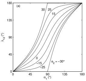
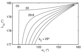
Figure 4: The variation of $\lambda_{12}$ as a function of $\alpha_{1}$ for $\phi_{1}=-30^{\circ}$, various $\phi_{2}$, and the WGS84 ellipsoid. Part (a) shows $\lambda_{12}$ for $\phi_{2}=0^{\circ}$, $\pm 15^{\circ}$, $\pm 25^{\circ}$, and $\pm 30^{\circ}$. For $\left|\phi_{2}\right|<\left|\phi_{1}\right|$, the curves are strictly increasing, while for $\phi_{2}=\pm\phi_{1}$, the curves are non-decreasing with discontinuities in the slopes at $\alpha_{1}=90^{\circ}$. An enlargement of the top right corner of (a) is shown in (b) with $\phi_{2}\in[29^{\circ},30^{\circ}]$ at intervals of $0.2^{\circ}$.

The solution of the hybrid geodesic problem is straightforward. Find $\beta_{1}$ and $\beta_{2}$ from Eq. (6), solve for $\alpha_{0}$ and $\alpha_{2}$ from Eq. (5), taking $\cos\alpha_{0}>0$ and $\cos\alpha_{2}\geq 0$. In order to compute $\alpha_{2}$ accurately, use

$$\cos\alpha_{2}=\frac{+\sqrt{\cos^{2}\alpha_{1}\cos^{2}\beta_{1}+(\cos^{2}\beta_{2}-\cos^{2}\beta_{1})}}{\cos\beta_{2}},$$ (45)

in addition to Eq. (5). Compute $\sigma_{1}$, $\omega_{1}$, $\sigma_{2}$, and $\omega_{2}$ using Eqs. (11) and (12). Finally, determine $\lambda_{12}$ (and, once convergence is achieved, $s_{12}$) as in the solution to the direct problem. The behavior of $\lambda_{12}$ as a function of $\alpha_{1}$ is shown in Fig. 4.

To apply Newton’s method, an expression for $\mathrm{d}\lambda_{12}/\mathrm{d}\alpha_{1}$ is needed. Consider a geodesic with initial azimuth $\alpha_{1}$. If the azimuth is increased to $\alpha_{1}+\mathrm{d}\alpha_{1}$ with its length held fixed, then the other end of the geodesic moves by $m_{12}\,\mathrm{d}\alpha_{1}$ in a direction $\frac{1}{2}\pi+\alpha_{2}$. If the geodesic is extended to intersect the parallel $\phi_{2}$ once more, the point of intersection moves by $m_{12}\,\mathrm{d}\alpha_{1}/\cos\alpha_{2}$; see Fig. 5. The radius of this parallel is $a\cos\beta_{2}$; thus the rate of change of the longitude difference is

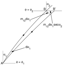
Figure 5: Finding $\mathrm{d}\lambda_{12}/\mathrm{d}\alpha_{1}$ with $\phi_{1}$ and $\phi_{2}$ held fixed.

$$\frac{\mathrm{d}\lambda_{12}}{\mathrm{d}\alpha_{1}}=\frac{m_{12}}{a}\frac{1}{\cos\alpha_{2}\cos\beta_{2}}.$$ (46)

This equation can also be obtained from Eq. (6.9.8b) of Helmert (1880). Equation (46) becomes indeterminate when $\beta_{2}=\pm\beta_{1}$ and $\alpha_{1}=\frac{1}{2}\pi$, because $m_{12}$ and $\cos\alpha_{2}$ both vanish. In this case, it is necessary to let $\alpha_{1}=\frac{1}{2}\pi+\delta$ and to take the limit $\delta\rightarrow\pm 0$, which gives

$$\frac{\mathrm{d}\lambda_{12}}{\mathrm{d}\alpha_{1}}=-\frac{\sqrt{1-e^{2}\cos^{2}\beta_{1}}}{\sin\beta_{1}}\bigl{(}1\mp\mathop{\mathrm{sign}}\nolimits(\cos\alpha_{1})\bigr{)},$$ (47)

where $\mathop{\mathrm{sign}}\nolimits(\cos\alpha_{1})=-\mathop{\mathrm{sign}}\nolimits(\delta)$. A numerical example of solving the inverse geodesic problem by this method is given at the end of the next section.

Vincenty (1975a), who uses the iterative method of Helmert (1880, §5.13) to solve the inverse problem, was aware of its failure to converge for nearly antipodal points. In an unpublished report (Vincenty, 1975b), he gives a modification of his method which deals with this case. Unfortunately, this sometimes requires many thousands of iterations to converge, whereas Newton’s method as described here only requires a few iterations.

5 Starting point for Newton’s method

Table 3: First sample inverse calculation specified by $\phi_{1}=-30.123\,45^{\circ}$, $\phi_{2}=-30.123\,44^{\circ}$, and $\lambda_{12}=0.000\,05^{\circ}$. Because the points are not nearly antipodal, an initial guess for $\alpha_{1}$ is found assuming $\omega_{12}=\lambda_{12}/\bar{w}$. However, in this case, the line is short enough that the error in $\omega_{12}$ is negligible at the precision given and the solution of the inverse problem is completed by using $s_{12}=a\bar{w}\sigma_{12}$. More generally, the value of $\alpha_{1}$ would be refined using Newton’s method.

Qty.	Value	Eq.
$\phi_{1}$	$-30.123\,45^{\circ}$	given
$\phi_{2}$	$-30.123\,44^{\circ}$	given
$\mbox{}\quad\lambda_{12}\quad\mbox{}$	$\hphantom{-0}0.000\,05^{\circ}$	given
Determine $\omega_{12}$
$\beta_{1}$	$-30.039\,990\,838\,21^{\circ}$	(6)
$\beta_{2}$	$-30.039\,980\,854\,91^{\circ}$	(6)
$\bar{w}$	$\hphantom{-0}0.997\,488\,477\,44$	(48)
$\omega_{12}$	$\hphantom{-0}0.000\,050\,125\,89^{\circ}$	$\lambda_{12}/\bar{w}$
$\sigma_{12}$	$\hphantom{-0}0.000\,044\,526\,41^{\circ}$	(51)
Solution
$\alpha_{1}$	$\hphantom{-}77.043\,533\,542\,37^{\circ}$	(49)
$\alpha_{2}$	$\hphantom{-}77.043\,508\,449\,13^{\circ}$	(50)
$s_{12}$	$\hphantom{-0}4.944\,208\,\mathrm{m}$	$a\bar{w}\sigma_{12}$

To complete the solution of the inverse problem a good starting guess for $\alpha_{1}$ is needed. In most cases, this is provided by assuming that $\omega_{12}=\lambda_{12}/\bar{w}$, where

$$\bar{w}=\sqrt{1-e^{2}\bigl{(}(\cos\beta_{1}+\cos\beta_{2})/2\bigr{)}^{2}}$$ (48)

and solving for the great circle on the auxiliary sphere, using (Vincenty, 1975a)

$$z_{1} =\cos\beta_{1}\sin\beta_{2}-\sin\beta_{1}\cos\beta_{2}\cos\omega_{12}$$

$$\qquad+i\cos\beta_{2}\sin\omega_{12},$$

$$z_{2} =-\sin\beta_{1}\cos\beta_{2}+\cos\beta_{1}\sin\beta_{2}\cos\omega_{12}$$

$$\qquad+i\cos\beta_{1}\sin\omega_{12},$$

$$\alpha_{1} =\mathop{\mathrm{ph}}\nolimits z_{1},$$ (49)

$$\alpha_{2} =\mathop{\mathrm{ph}}\nolimits z_{2},$$ (50)

$$\sigma_{12} =\mathop{\mathrm{ph}}\nolimits(\sin\beta_{1}\sin\beta_{2}+\cos\beta_{1}\cos\beta_{2}\cos\omega_{12}+i\left|z_{1}\right|).$$ (51)

An example of the solution of the inverse problem by this method is given in Table 3.

This procedure is inadequate for nearly antipodal points because both the real and imaginary components of $z_{1}$ are small and $\alpha_{1}$ depends very sensitively on $\omega_{12}$. In the corresponding situation on the sphere, it is possible to determine $\alpha_{1}$ by noting that all great circles emanating from $A$ meet at $O$, the point antipodal to $A$. Thus $\alpha_{1}$ may be determined as the supplement of the azimuth of the great circle $BO$ at $O$; in addition, because $B$ and $O$ are close, it is possible to approximate the sphere, locally, as a plane.

The situation for an ellipsoid is slightly different because the geodesics emanating from $A$, instead of meeting at a point, form an envelope, centered at $O$, in the shape of an astroid whose extent is $O(f)$ (Jacobi, 1891, Eqs. (16)–(17)). The position at which a particular geodesic touches this envelope is given by the condition $m_{12}=0$. However elementary methods can be used to determine the envelope. Consider a geodesic leaving $A$ (with $\beta_{1}\leq 0$) with azimuth $\alpha_{1}\in[{\textstyle\frac{1}{2}}\pi,\pi]$. This first intersects the circle of opposite latitude, $\beta_{2}=-\beta_{1}$, with $\sigma_{12}=\omega_{12}=\pi$ and $\alpha_{2}=\pi-\alpha_{1}$. Equation  (8) then gives

$$\lambda_{12}=\pi-f\pi\cos\beta_{1}\sin\alpha_{1}+O(f^{2}).$$ (52)

Define a plane coordinate system $(x,y)$ centered on the antipodal point where $\Delta=fa\pi\cos^{2}\beta_{1}$ is the unit of length, i.e.,

$$\lambda_{12}=\pi+\frac{\Delta}{a\cos\beta_{1}}x,\quad\beta_{2}=-\beta_{1}+\frac{\Delta}{a}y.$$ (53)

In this coordinate system, Eq. (52) corresponds to the point $x=-\sin\alpha_{1}$, $y=0$ and the slope of the geodesic is $-\cot\alpha_{1}$. Thus, in the neighborhood of the antipodal point, the geodesic may be approximated by

$$\frac{x}{\sin\alpha_{1}}+\frac{y}{\cos\alpha_{1}}+1=0,$$ (54)

where terms of order $f^{2}$ have been neglected. Allowing $\alpha_{1}$ to vary, Eq. (54) defines a family of lines approximating the geodesics emanating from $A$. Differentiating this equation with respect to $\alpha_{1}$ and solving the resulting pair of equations for $x$ and $y$ gives the parametric equations for the astroid, $x=-\sin^{3}\alpha_{1}$, and $y=-\cos^{3}\alpha_{1}$. Note that, for the ordering of points given by Eq. (44), $x\leq 0$ and $y\leq 0$.

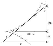
Figure 6: The solution of the astroid equations by similar triangles. The scaled coordinates of $B$ are $(x,y)$; $O$ is the point antipodal to $A$. The line $BCD$, which is given by Eq. (54), is the continuation of the geodesic from $AB$ with $C$ being its intersection with the circle $\beta=-\beta_{1}$ and $D$ its intersection with the meridian $\lambda=\lambda_{1}+\pi$. The envelope of lines satisfying $CD=1$ gives the astroid, a portion of which is shown by the curves.

Given $x$ and $y$ (i.e., the position of point $B$), Eq. (54) may be solved to obtain a first approximation to $\alpha_{1}$. This prescription is given by Helmert (1880, Eq. (7.3.7)) who notes that this results in a quartic which may be found using the construction given in Fig. 6. Here $COD$ and $BED$ are similar triangles; if the (signed) length $BC$ is $\mu$, then an equation for $\mu$ can be found by applying Pythagoras’ theorem to $COD$,

$$\frac{x^{2}}{(1+\mu)^{2}}+\frac{y^{2}}{\mu^{2}}=1,$$

which can be expanded to give a 4th-order polynomial in $\mu$,

$$\mu^{4}+2\mu^{3}+(1-x^{2}-y^{2})\mu^{2}-2y^{2}\mu-y^{2}=0.$$ (55)

Table 4: Second sample inverse calculation specified by $\phi_{1}=-30^{\circ}$, $\phi_{2}=29.9^{\circ}$, and $\lambda_{12}=179.8^{\circ}$. Because the points are nearly antipodal, an initial guess for $\alpha_{1}$ is found by solving the astroid problem. Here $\mu$ is the positive root of Eq. (55). If $y=0$, then $\alpha_{1}$ is given by Eq. (57). The value of $\alpha_{1}$ is used in Table 5.

Qty.	Value	Eq.
$\phi_{1}$	$-30^{\circ}$	given
$\phi_{2}$	$\hphantom{0}\hbox{}29.9^{\circ}$	given
$\mbox{}\quad\lambda_{12}\quad\mbox{}$	$\hbox{}179.8^{\circ}$	given
Solve the astroid problem
$x$	$-0.382\,344$	(53)
$y$	$-0.220\,189$	(53)
$\mu$	$\hphantom{-}0.231\,633$	(55)
Initial guess for $\alpha_{1}$
$\alpha_{1}$	$\hbox{}161.914^{\circ}$	(56)

Descartes’ rule of signs shows that, for $y\neq 0$, there is one positive root (Olver et al., 2010, §http://dlmf.nist.gov/1.11.ii) and this is the solution corresponding to the shortest path. This root can be found by standard methods (Olver et al., 2010, §http://dlmf.nist.gov/1.11.iii). Equation (55) arises in converting from geocentric to geodetic coordinates, and I use the solution to that problem given by Vermeille (2002). The azimuth can then be determined from the triangle $COD$ in Fig. 6,

$$\alpha_{1}=\mathop{\mathrm{ph}}\nolimits\bigl{(}y/\mu-ix/(1+\mu)\bigr{)}.$$ (56)

If $y=0$, the solution is found by taking the limit $y\rightarrow 0$,

$$\alpha_{1}=\mathop{\mathrm{ph}}\nolimits\bigl{(}\pm\sqrt{\max(0,1-x^{2})}-ix\bigr{)}.$$ (57)

Tables 4–6 together illustrate the complete solution of the inverse problem for nearly antipodal points.

Table 5: Second sample inverse calculation, continued. Here $\lambda_{12}^{(0)}$ denotes the desired value of the longitude difference; Newton’s method is used to adjust $\alpha_{1}$ so that $\lambda_{12}=\lambda_{12}^{(0)}$. The final value of $\alpha_{1}$ is used in Table 6.

Qty.	Value	Eq.
$\phi_{1}$	$-30^{\circ}$	given
$\phi_{2}$	$\hphantom{-}29.9^{\circ}$	given
$\alpha_{1}$	$\hbox{}161.914^{\circ}$	Table 4
$\lambda_{12}^{(0)}$	$\hbox{}179.8^{\circ}$	given
Solve triangle $N\!EA$
$\beta_{1}$	$\hphantom{0}{-29.916\,747\,713\,24^{\circ}}$	(6)
$\alpha_{0}$	$\hphantom{-0}15.609\,397\,464\,14^{\circ}$	(10)
$\sigma_{1}$	$-148.812\,535\,665\,96^{\circ}$	(11)
$\omega_{1}$	$-170.748\,966\,961\,28^{\circ}$	(12)
Solve triangle $N\!EB$
$\beta_{2}$	$\hphantom{-0}29.816\,916\,421\,89^{\circ}$	(6)
$\alpha_{2}$	$\hphantom{-0}18.067\,287\,962\,31^{\circ}$	(5), (45)
$\sigma_{2}$	$\hphantom{-0}31.082\,449\,768\,95^{\circ}$	(11)
$\omega_{2}$	$\hphantom{-00}9.213\,457\,611\,10^{\circ}$	(12)
Determine $\lambda_{12}$
$k^{2}$	$\hphantom{0}0.006\,251\,537\,916\,62$	(9)
$\epsilon$	$\hphantom{0}0.001\,558\,018\,267\,80$	(16)
$\lambda_{1}$	$-170.614\,835\,524\,58^{\circ}$	(8)
$\lambda_{2}$	$\hphantom{-00}9.185\,420\,098\,39^{\circ}$	(8)
$\lambda_{12}$	$\hphantom{-}179.800\,255\,622\,97^{\circ}$	$\lambda_{2}-\lambda_{1}$
Update $\alpha_{1}$
$\delta\lambda_{12}$	$\hphantom{-}0.000\,255\,622\,97^{\circ}$	$\lambda_{12}-\lambda_{12}^{(0)}$
$J(\sigma_{1})$	$-0.009\,480\,409\,276\,40$	(3)
$J(\sigma_{2})$	$\hphantom{-}0.000\,313\,491\,286\,30$	(3)
$m_{12}$	$\hphantom{-}57\,288.000\,110\,\mathrm{m}$	(38)
$\mathrm{d}\lambda_{12}/\mathrm{d}\alpha_{1}$	$\hphantom{0}0.010\,889\,317\,161\,15$	(46)
$\delta\alpha_{1}$	$\hphantom{0}{-0.023\,474\,655\,19^{\circ}}$	$-\delta\lambda_{12}/(\mathrm{d}\lambda_{12}/\mathrm{d}\alpha_{1})$
$\alpha_{1}$	$\hbox{}161.890\,525\,344\,81^{\circ}$	$\alpha_{1}+\delta\alpha_{1}$
Next iteration
$\delta\lambda_{12}$	$\hphantom{00}0.000\,000\,006\,63^{\circ}$
$\alpha_{1}$	$161.890\,524\,736\,33^{\circ}$

Table 6: Second sample inverse calculation, concluded. Here the hybrid problem ($\phi_{1}$, $\phi_{2}$, and $\alpha_{1}$ given) is solved. The computed value of $\lambda_{12}$ matches that given in the specification of the inverse problem in Table 4.

Qty.	Value	Eq.
$\phi_{1}$	$-30^{\circ}$	given
$\phi_{2}$	$\hphantom{-}29.9^{\circ}$	given
$\alpha_{1}$	$\hbox{}161.890\,524\,736\,33^{\circ}$	Table 5
Solve triangle $N\!EA$
$\beta_{1}$	$\hphantom{0}{-29.916\,747\,713\,24^{\circ}}$	(6)
$\alpha_{0}$	$\hphantom{-0}15.629\,479\,665\,37^{\circ}$	(10)
$\sigma_{1}$	$-148.809\,136\,917\,76^{\circ}$	(11)
$\omega_{1}$	$-170.736\,343\,780\,66^{\circ}$	(12)
Solve triangle $N\!EB$
$\beta_{2}$	$\hphantom{-0}29.816\,916\,421\,89^{\circ}$	(6)
$\alpha_{2}$	$\hphantom{-0}18.090\,737\,245\,74^{\circ}$	(5), (45)
$\sigma_{2}$	$\hphantom{-0}31.085\,834\,470\,40^{\circ}$	(11)
$\omega_{2}$	$\hphantom{-00}9.226\,028\,621\,10^{\circ}$	(12)
Determine $s_{12}$ and $\lambda_{12}$
$s_{1}$	$-16\,539\,979.064\,227\,\mathrm{m}$	(7)
$s_{2}$	$\hphantom{-0}3\,449\,853.763\,383\,\mathrm{m}$	(7)
$s_{12}$	$\hphantom{-}19\,989\,832.827\,610\,\mathrm{m}$	$s_{2}-s_{1}$
$\lambda_{1}$	$-170.602\,047\,121\,48^{\circ}$	(8)
$\lambda_{2}$	$\hphantom{-00}9.197\,952\,878\,52^{\circ}$	(8)
$\mbox{}\quad\lambda_{12}\quad\mbox{}$	$\hphantom{-}179.800\,000\,000\,00^{\circ}$	$\lambda_{2}-\lambda_{1}$
Solution
$\alpha_{1}$	$161.890\,524\,736\,33^{\circ}$
$\alpha_{2}$	$\hphantom{0}18.090\,737\,245\,74^{\circ}$
$s_{12}$	$19\,989\,832.827\,610\,\mathrm{m}$

6 Area

The last geodesic algorithm I present is for geodesic areas. Here, I extend the method of Danielsen (1989) to higher order so that the result is accurate to round-off, and I recast his series into a simple trigonometric sum.

Let $S_{12}$ be the area of the geodesic quadrilateral $AF\!H\!B$ in Fig. 1. Following Danielsen (1989), this can be expressed as the sum of a spherical term and an integral giving the ellipsoidal correction,

$$S_{12} =S(\sigma_{2})-S(\sigma_{1}),$$ (58)

$$S(\sigma) =c^{2}\alpha+e^{2}a^{2}\cos\alpha_{0}\sin\alpha_{0}\,I_{4}(\sigma),$$ (59)

where

$$c^{2}=\frac{a^{2}}{2}+\frac{b^{2}}{2}\frac{\tanh^{-1}e}{e}$$ (60)

is the authalic radius,

$$I_{4}(\sigma) =-\int_{\pi/2}^{\sigma}\frac{t(e^{\prime 2})-t(k^{2}\sin^{2}\sigma^{\prime})}{e^{\prime 2}-k^{2}\sin^{2}\sigma^{\prime}}\frac{\sin\sigma^{\prime}}{2}\,\mathrm{d}\sigma^{\prime},$$ (61)

$$t(x) =x+\sqrt{x^{-1}+1}\,\sinh^{-1}\!\sqrt{x}.$$

Expanding the integrand in powers of $e^{\prime 2}$ and $k^{2}$ and performing the integral gives

$$I_{4}(\sigma)=\sum_{l=0}^{\infty}C_{4l}\cos\bigl{(}(2l+1)\sigma\bigr{)},$$ (62)

where

$$C_{40} =\bigl{(}{\textstyle\frac{2}{3}}-{\textstyle\frac{1}{15}}e^{\prime 2}+{\textstyle\frac{4}{105}}e^{\prime 4}-{\textstyle\frac{8}{315}}e^{\prime 6}+{\textstyle\frac{64}{3465}}e^{\prime 8}-{\textstyle\frac{128}{9009}}e^{\prime 10}\bigr{)}$$

$$\quad-\bigl{(}{\textstyle\frac{1}{20}}-{\textstyle\frac{1}{35}}e^{\prime 2}+{\textstyle\frac{2}{105}}e^{\prime 4}-{\textstyle\frac{16}{1155}}e^{\prime 6}+{\textstyle\frac{32}{3003}}e^{\prime 8}\bigr{)}k^{2}$$

$$\quad+\bigl{(}{\textstyle\frac{1}{42}}-{\textstyle\frac{1}{63}}e^{\prime 2}+{\textstyle\frac{8}{693}}e^{\prime 4}-{\textstyle\frac{80}{9009}}e^{\prime 6}\bigr{)}k^{4}$$

$$\quad-\bigl{(}{\textstyle\frac{1}{72}}-{\textstyle\frac{1}{99}}e^{\prime 2}+{\textstyle\frac{10}{1287}}e^{\prime 4}\bigr{)}k^{6}$$

$$\quad+\bigl{(}{\textstyle\frac{1}{110}}-{\textstyle\frac{1}{143}}e^{\prime 2}\bigr{)}k^{8}-{\textstyle\frac{1}{156}}k^{10}+\cdots,$$

$$C_{41} =\bigl{(}{\textstyle\frac{1}{180}}-{\textstyle\frac{1}{315}}e^{\prime 2}+{\textstyle\frac{2}{945}}e^{\prime 4}-{\textstyle\frac{16}{10395}}e^{\prime 6}+{\textstyle\frac{32}{27027}}e^{\prime 8}\bigr{)}k^{2}$$

$$\quad-\bigl{(}{\textstyle\frac{1}{252}}-{\textstyle\frac{1}{378}}e^{\prime 2}+{\textstyle\frac{4}{2079}}e^{\prime 4}-{\textstyle\frac{40}{27027}}e^{\prime 6}\bigr{)}k^{4}$$

$$\quad+\bigl{(}{\textstyle\frac{1}{360}}-{\textstyle\frac{1}{495}}e^{\prime 2}+{\textstyle\frac{2}{1287}}e^{\prime 4}\bigr{)}k^{6}$$

$$\quad-\bigl{(}{\textstyle\frac{1}{495}}-{\textstyle\frac{2}{1287}}e^{\prime 2}\bigr{)}k^{8}+{\textstyle\frac{5}{3276}}k^{10}+\cdots,$$

$$C_{42} =\bigl{(}{\textstyle\frac{1}{2100}}-{\textstyle\frac{1}{3150}}e^{\prime 2}+{\textstyle\frac{4}{17325}}e^{\prime 4}-{\textstyle\frac{8}{45045}}e^{\prime 6}\bigr{)}k^{4}$$

$$\quad-\bigl{(}{\textstyle\frac{1}{1800}}-{\textstyle\frac{1}{2475}}e^{\prime 2}+{\textstyle\frac{2}{6435}}e^{\prime 4}\bigr{)}k^{6}$$

$$\quad+\bigl{(}{\textstyle\frac{1}{1925}}-{\textstyle\frac{2}{5005}}e^{\prime 2}\bigr{)}k^{8}-{\textstyle\frac{1}{2184}}k^{10}+\cdots,$$

$$C_{43} =\bigl{(}{\textstyle\frac{1}{17640}}-{\textstyle\frac{1}{24255}}e^{\prime 2}+{\textstyle\frac{2}{63063}}e^{\prime 4}\bigr{)}k^{6}$$

$$\quad-\bigl{(}{\textstyle\frac{1}{10780}}-{\textstyle\frac{1}{14014}}e^{\prime 2}\bigr{)}k^{8}+{\textstyle\frac{5}{45864}}k^{10}+\cdots,$$

$$C_{44} =\bigl{(}{\textstyle\frac{1}{124740}}-{\textstyle\frac{1}{162162}}e^{\prime 2}\bigr{)}k^{8}-{\textstyle\frac{1}{58968}}k^{10}+\cdots,$$

$$C_{45} ={\textstyle\frac{1}{792792}}k^{10}+\cdots.$$ (63)

Table 7: The calculation of the area between the equator and the geodesic specified by $\phi_{1}=40^{\circ}$, $\alpha_{1}=30^{\circ}$, and $s_{12}=10\,000\,\mathrm{km}$. This uses intermediate values computed in Table 2.

Qty.	Value	Eq.
$\alpha_{0}$	$\hphantom{0}22.553\,940\,202\,62^{\circ}$	Table 2
$\alpha_{1}$	$\hphantom{0}30^{\circ}$	Table 2
$\alpha_{2}$	$149.090\,169\,318\,07^{\circ}$	Table 2
$\sigma_{1}$	$\hphantom{0}43.999\,153\,645\,00^{\circ}$	Table 2
$\sigma_{2}$	$133.921\,640\,830\,38^{\circ}$	Table 2
$k^{2}$	$0.005\,748\,029\,628\,57$	Table 2
Compute area
$I_{4}(\sigma_{1})$	$\hphantom{-}0.479\,018\,145\,20$	(62)
$I_{4}(\sigma_{2})$	$-0.461\,917\,119\,02$	(62)
$S(\sigma_{1})$	$\hphantom{0}21\,298\,942.667\,15\,\mathrm{km}^{2}$	(59)
$S(\sigma_{2})$	$105\,574\,566.089\,50\,\mathrm{km}^{2}$	(59)
$S_{12}$	$\hphantom{0}84\,275\,623.422\,35\,\mathrm{km}^{2}$	(58)

An example of the computation of $S_{12}$ is given in Table 7.

Summing $S_{12}$, Eq. (58), over the edges of a geodesic polygon gives the area of the polygon provided that it does not encircle a pole; if it does, $2\pi c^{2}$ should be added to the result. The first term in Eq. (59) contributes $c^{2}(\alpha_{2}-\alpha_{1})$ to $S_{12}$. This is the area of the quadrilateral $AF\!H\!B$ on a sphere of radius $c$ and it is proportional to its spherical excess, $\alpha_{2}-\alpha_{1}$, the sum of its interior angles less $2\pi$. It is important that this term be computed accurately when the edge is short (and $\alpha_{1}$ and $\alpha_{2}$ are nearly equal). A suitable identity for $\alpha_{2}-\alpha_{1}$ is given by Bessel (1825, §11),

$$\tan\frac{\alpha_{2}-\alpha_{1}}{2}=\frac{\sin{\textstyle\frac{1}{2}}(\beta_{2}+\beta_{1})}{\cos{\textstyle\frac{1}{2}}(\beta_{2}-\beta_{1})}\tan\frac{\omega_{12}}{2}.$$ (64)

7 Implementation

The algorithms described in the preceding sections can be readily converted into working code. The polynomial expansions, Eqs. (17), (18), (21), (24), (25), (42), (43), and (6), are such that the final results are accurate to $O(f^{6})$ which means that, even for $f=\frac{1}{150}$, the truncation error is smaller than the round-off error when using IEEE double precision arithmetic (with the fraction of the floating point number represented by 53 bits). For speed and to minimize round-off errors, the polynomials should be evaluated with the Horner method. The parenthetical expressions in Eqs. (24), (25), and (6) depend only on the flattening of the ellipsoid and can be computed once this is known. When determining many points along a single geodesic, the polynomials need be evaluated just once. Clenshaw (1955) summation should be used to sum the Fourier series, Eqs. (15), (23), (41), and (62).

There are several other details to be dealt with in implementing the algorithms: where to apply the two rules for choosing starting points for Newton’s method, a slight improvement to the starting guess Eq. (56), the convergence criterion for Newton’s method, how to minimize round-off errors in solving the trigonometry problems on the auxiliary sphere, rapidly computing intermediate points on a geodesic by using $\sigma_{12}$ as the metric, etc. I refer the reader to the implementations of the algorithms in GeographicLib (Karney, 2012) for possible ways to address these issues. The C++ implementation has been tested against a large set of geodesics for the WGS84 ellipsoid; this was generated by continuing the series expansions to $O(f^{30})$ and by solving the direct problem using with high-precision arithmetic. The round-off errors in the direct and inverse methods are less than 15 nanometers and the error in the computation of the area $S_{12}$ is about $0.1\,\mathrm{m^{2}}$. Typically, 2 to 4 iterations of Newton’s method are required for convergence, although in a tiny fraction of cases up to 16 iterations are required. No convergence failures are observed. With the C++ implementation compiled with the g++ compiler, version 4.4.4, and running on a $2.66\,\mathrm{GHz}$ Intel processor, solving the direct geodesic problem takes $0.88\,\mathrm{\mu s}$, while the inverse problem takes $2.34\,\mathrm{\mu s}$ (on average). Several points along a geodesic can be computed at the rate of $0.37\,\mathrm{\mu s}$ per point. These times are comparable to those for Vincenty’s algorithms implemented in C++ and run on the same architecture: $1.11\,\mathrm{\mu s}$ for the direct problem and $1.34\,\mathrm{\mu s}$ for the inverse problem. (But note that Vincenty’s algorithms are less accurate than those given here and that his method for the inverse problem sometimes fails to converge.)

8 Ellipsoidal gnomonic projection

As an application of the differential properties of geodesics, I derive a generalization of the gnomonic projection to the ellipsoid. The gnomonic projection of the sphere has the property that all geodesics on the sphere map to straight lines (Snyder, 1987, §22). Such a projection is impossible for an ellipsoid because it does not have constant Gaussian curvature (Beltrami, 1865, §18); nevertheless, a projection can be constructed in which geodesics are very nearly straight.

The spherical gnomonic projection is the limit of the doubly azimuthal projection of the sphere, wherein the bearings from two fixed points $A$ and $A^{\prime}$ to $B$ are preserved, as $A^{\prime}$ approaches $A$ (Bugayevskiy and Snyder, 1995). The construction of the generalized gnomonic projection proceeds in the same way; see Fig. 7. Draw a geodesic $A^{\prime}B^{\prime}$ such that it is parallel to the geodesic $AB$ at $A$. Its initial separation from $AB$ is $\sin\gamma\,\mathrm{d}t$; at $B^{\prime}$, the point closest to $B$, the separation becomes $M_{12}\sin\gamma\,\mathrm{d}t$ (in the limit $\mathrm{d}t\rightarrow 0$). Thus the difference in the azimuths of the geodesics $A^{\prime}B$ and $A^{\prime}B^{\prime}$ at $A^{\prime}$ is $(M_{12}/m_{12})\sin\gamma\,\mathrm{d}t$, which gives $\gamma+\gamma^{\prime}=\pi-(M_{12}/m_{12})\sin\gamma\,\mathrm{d}t$. Now, solving the planar triangle problem with $\gamma$ and $\gamma^{\prime}$ as the two base angles gives the distance $AB$ on the projection plane as $m_{12}/M_{12}$.

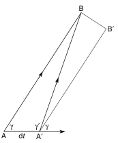
Figure 7: The construction of the generalized gnomonic projection as the limit of a doubly azimuthal projection.

This leads to the following specification for the generalized gnomonic projection. Let the center point be $A$; for an arbitrary point $B$, solve the inverse geodesic problem between $A$ and $B$; then $B$ projects to the point

$$x=\rho\sin\alpha_{1},\quad y=\rho\cos\alpha_{1},\quad\rho=m_{12}/M_{12};$$ (65)

the projection is undefined if $M_{12}\leq 0$. In the spherical limit, this becomes the standard gnomonic projection, $\rho=a\tan\sigma_{12}$ (Snyder, 1987, p. 165). The azimuthal scale is $1/M_{12}$ and the radial scale, found by taking the derivative $\mathrm{d}\rho/\mathrm{d}s_{12}$ and using Eq. (28), is $1/M_{12}^{2}$. The reverse projection is found by computing $\alpha_{1}=\mathop{\mathrm{ph}}\nolimits(y+ix)$, finding $s_{12}$ using Newton’s method with $\mathrm{d}\rho/\mathrm{d}s_{12}=1/M_{12}^{2}$ (i.e., the radial scale), and solving the resulting direct geodesic problem.

In order to gauge the usefulness of the ellipsoidal gnomonic projection, consider two points on the earth $B$ and $C$, map these points to the projection, and connect them with a straight line in this projection. If this line is mapped back onto the surface of the earth, it will deviate slightly from the geodesic $BC$. To lowest order, the maximum deviation $\mathbf{h}$ occurs at the midpoint of the line segment $BC$; empirically, I find

$$\mathbf{h}=\frac{l^{2}}{32}(\nabla K\cdot\mathbf{t})\mathbf{t},$$ (66)

where $l$ is the length of the geodesic, $K$ is the Gaussian curvature, $\nabla K$ is evaluated at the center of the projection $A$, and $\mathbf{t}$ is the perpendicular vector from the center of projection to the geodesic. The deviation in the azimuths at the end points is about $4h/l$ and the length is greater than the geodesic distance by about $\frac{8}{3}h^{2}/l$. In the case of an ellipsoid of revolution, the curvature is given by differentiating Eq. (37) with respect to $\phi$ and dividing by the meridional radius of curvature to give

$$\nabla K=-\frac{4a}{b^{4}}e^{2}(1-e^{2}\sin^{2}\phi)^{5/2}\cos\phi\sin\phi\,\mathbf{\hat{\boldsymbol{\phi}}},$$ (67)

where $\mathbf{\hat{\boldsymbol{\phi}}}$ is a unit vector pointing north. Bounding the magnitude of $\mathbf{h}$, Eq. (66), over all the geodesics whose end points lie within a distance $r$ of the center of projection, gives (in the limit that $f$ and $r$ are small)

$$\frac{h}{r}\leq\frac{f}{8}\frac{r^{3}}{a^{3}}.$$ (68)

The maximum value is attained when the center of projection is at $\phi=\pm 45^{\circ}$ and the geodesic is running in an east-west direction with the end points at bearings $\pm 45^{\circ}$ or $\pm 135^{\circ}$ from the center.

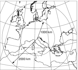
Figure 8: The coast line of Europe and North Africa in the ellipsoidal gnomonic projection with center at $(45^{\circ}\mathrm{N},12^{\circ}\mathrm{E})$ near Venice. The graticule lines are shown at multiples of $10^{\circ}$. The two circles are centered on the projection center with (geodesic) radii of $1000\,\mathrm{km}$ and $2000\,\mathrm{km}$. The data for the coast lines is taken from GMT (Wessel and Smith, 2010) at “low” resolution.

Others have proposed different generalizations of the gnomonic projection. Bowring (1997) and Williams (1997) give a projection in which great ellipses project to straight lines; Letoval’tsev (1963) suggests a projection in which normal sections through the center point map to straight lines. Empirically, I find that $h/r$ is proportional to $r/a$ and $r^{2}/a^{2}$ for these projections. Thus, neither does as well as the projection derived above (for which $h/r$ is proportional to $r^{3}/a^{3}$) at preserving the straightness of geodesics.

As an illustration of the properties of the ellipsoidal gnomonic projection, Eq. (65), consider Fig. 8 in which a projection of Europe is shown. The two circles are geodesic circles of radii $1000\,\mathrm{km}$ and $2000\,\mathrm{km}$. If the geodesic between any two points within one of these circles is estimated by using a straight line on this figure, the deviation from the true geodesic is less than $1.7\,\mathrm{m}$ and $28\,\mathrm{m}$, respectively. The maximum errors in the end azimuths are $1.1^{\prime\prime}$ and $8.6^{\prime\prime}$ and the maximum errors in the lengths are only $5.4\,\mu\mathrm{m}$ and $730\,\mu\mathrm{m}$.

The gnomonic projection can be used to solve two geodesic problems accurately and rapidly. The first is the intersection problem: given two geodesics between $A$ and $B$ and between $C$ and $D$, determine the point of intersection, $O$. This can be solved as follows. Guess an intersection point $O^{(0)}$ and use this as the center of the gnomonic projection; define $\mathbf{a}$, $\mathbf{b}$, $\mathbf{c}$, $\mathbf{d}$ as the positions of $A$, $B$, $C$, $D$ in the projection; find the intersection of $AB$ and $CD$ in the projection, i.e.,

$$\mathbf{o}=\frac{(\mathbf{c}\times\mathbf{d}\cdot\mathbf{\hat{z}})(\mathbf{b}-\mathbf{a})-(\mathbf{a}\times\mathbf{b}\cdot\mathbf{\hat{z}})(\mathbf{d}-\mathbf{c})}{(\mathbf{b}-\mathbf{a})\times(\mathbf{d}-\mathbf{c})\cdot\mathbf{\hat{z}}},$$ (69)

where $\mathbf{\hat{\text{\ }}}$ indicates a unit vector ($\mathbf{\hat{a}}=\mathbf{a}/a$) and $\mathbf{\hat{z}}=\mathbf{\hat{x}}\times\mathbf{\hat{y}}$ is in the direction perpendicular to the projection plane. Project $\mathbf{o}$ back to geographic coordinates $O^{(1)}$ and use this as a new center of projection; iterate this process until $O^{(i)}=O^{(i-1)}$ which is then the desired intersection point.

The second problem is the interception problem: given a geodesic between $A$ and $B$, find the point $O$ on the geodesic which is closest to a given point $C$. The solution is similar to that for the intersection problem; however the interception point in the projection is

$$\mathbf{o}=\frac{\mathbf{c}\cdot(\mathbf{b}-\mathbf{a})(\mathbf{b}-\mathbf{a})-(\mathbf{a}\times\mathbf{b}\cdot\mathbf{\hat{z}})\mathbf{\hat{z}}\times(\mathbf{b}-\mathbf{a})}{\left|\mathbf{b}-\mathbf{a}\right|^{2}}.$$

Provided the given points lie within about a quarter meridian of the intersection or interception points (so that the gnomonic projection is defined), these algorithms converge quadratically to the exact result.

9 Conclusions

The classical geodesic problems entail solving the ellipsoidal triangle $N\!AB$ in Fig. 1, whose sides and angles are represented by $\phi_{1}$, $\phi_{2}$, $s_{12}$ and $\alpha_{1}$, $\alpha_{2}$, $\lambda_{12}$. In the direct problem $\phi_{1}$, $\alpha_{1}$, and $s_{12}$ are given, while in the inverse problem $\phi_{1}$, $\lambda_{12}$, and $\phi_{2}$ are specified; and the goal in each case is to solve for the remaining side and angles. The algorithms given here provide accurate, robust, and fast solutions to these problems; they also allow the differential and integral quantities $m_{12}$, $M_{12}$, $M_{21}$, and $S_{12}$ to be computed.

Much of the work described here involves applying standard computational techniques to earlier work. However, at least two aspects are novel: (1) This paper presents the first complete solution to the inverse geodesic problem. (2) The ellipsoidal gnomonic projection is a new tool to solve various geometrical problems on the ellipsoid.

Furthermore, the packaging of these various geodesic capabilities into a single library is also new. This offers a straightforward solution of several interesting problems. Two geodesic projections, the azimuthal equidistant projection and the Cassini-Soldner projection, are simple to write and their domain of applicability is not artificially restricted, as would be the case, for example, if the series expansion for the Cassini-Soldner projection were used (Snyder, 1987, §13); the scales for these projections are simply given in terms of $m_{12}$ and $M_{12}$. Several other problems can be readily tackled with this library, e.g., solving other ellipsoidal trigonometry problems and finding the median line and other maritime boundaries. These and other problems are explored in Karney (2011). The web page http://geographiclib.sf.net/geod.html provides additional information, including the Maxima (2009) code used to carry out the Taylor expansions and a JavaScript implementation which allows geodesic problems to be solved on many portable devices.

References

- Beltrami (1865) E. Beltrami, 1865, Risoluzione del problema: Riportare i punti di una superficie sopra un piano in modo che le linee geodetiche vengano rappresentate da linee rette, Annali Mat. Pura App., 7, 185–204, http://books.google.com/books?id=dfgEAAAAYAAJ&pg=PA185.
- Bessel (1825) F. W. Bessel, 1825, Über die Berechnung der geographischen Längen und Breiten aus geodätischen Vermessungen, Astron. Nachr., 4(86), 241–254, http://adsabs.harvard.edu/abs/1825AN……4..241B, translated into English by C. F. F. Karney and R. E. Deakin as The calculation of longitude and latitude from geodesic measurements, Astron. Nachr. 331(8), 852–861 (2010), http://dx.doi.org/10.1002/asna.201011352, E-print http://arxiv.org/abs/0908.1824.
- Bowring (1997) B. R. Bowring, 1997, The central projection of the spheroid and surface lines, Survey Review, 34(265), 163–173.
- Bugayevskiy and Snyder (1995) L. M. Bugayevskiy and J. P. Snyder, 1995, Map Projections: A Reference Manual (Taylor & Francis, London), http://www.worldcat.org/oclc/31737484.
- Christoffel (1868) E. B. Christoffel, 1868, Allgemeine Theorie der geodätischen Dreiecke, Math. Abhand. König. Akad. der Wiss. zu Berlin, 8, 119–176, http://books.google.com/books?id=EEtFAAAAcAAJ&pg=PA119.
- Clairaut (1735) A. C. Clairaut, 1735, Détermination géometrique de la perpendiculaire à la méridienne tracée par M. Cassini, Mém. de l’Acad. Roy. des Sciences de Paris 1733, pp. 406–416, http://books.google.com/books?id=GOAEAAAAQAAJ&pg=PA406.
- Clenshaw (1955) C. W. Clenshaw, 1955, A note on the summation of Chebyshev series, Math. Tables Aids Comput., 9(51), 118–120, http://www.jstor.org/stable/2002068.
- Danielsen (1989) J. S. Danielsen, 1989, The area under the geodesic, Survey Review, 30(232), 61–66.
- Gauss (1828) C. F. Gauss, 1828, Disquisitiones Generales circa Superficies Curvas (Dieterich, Göttingen), http://books.google.com/books?id=bX0AAAAAMAAJ, translated into English by J. C. Morehead and A. M. Hiltebeitel as General Investigations of Curved Surfaces of 1827 and 1825 (Princeton Univ. Lib., 1902), http://books.google.com/books?id=a1wTJR3kHwUC.
- Helmert (1880) F. R. Helmert, 1880, Die Mathematischen und Physikalischen Theorieen der Höheren Geodäsie, volume 1 (Teubner, Leipzig), http://books.google.com/books?id=qt2CAAAAIAAJ, translated into English by Aeronautical Chart and Information Center (St. Louis, 1964) as Mathematical and Physical Theories of Higher Geodesy, Part 1, http://geographiclib.sf.net/geodesic-papers/helmert80-en.html.
- Jacobi (1891) C. G. J. Jacobi, 1891, Über die Curve, welche alle von einem Punkte ausgehenden geodätischen Linien eines Rotationsellipsoides berührt, in K. T. W. Weierstrass, editor, Gesammelte Werke, volume 7, pp. 72–87 (Reimer, Berlin), op. post., completed by F. H. A. Wangerin, http://books.google.com/books?id=˙09tAAAAMAAJ&pg=PA72.
- Karney (2011) C. F. F. Karney, 2011, Geodesics on an ellipsoid of revolution, Technical report, SRI International, E-print http://arxiv.org/abs/1102.1215v1.
- Karney (2012) —, 2012, GeographicLib, version 1.20, http://geographiclib.sf.net.
- Legendre (1806) A. M. Legendre, 1806, Analyse des triangles tracés sur la surface d’un sphéroïde, Mém. de l’Inst. Nat. de France, 1st sem., pp. 130–161, http://books.google.com/books?id=-d0EAAAAQAAJ&pg=PA130-IA4.
- Letoval’tsev (1963) I. G. Letoval’tsev, 1963, Generalization of the gnomonic projection for a spheroid and the principal geodetic problems involved in the alignment of surface routes, Geodesy and Aerophotography, 5, 271–274, translation of Geodeziya i Aerofotos’emka 5, 61–68 (1963).
- Maxima (2009) Maxima, 2009, A computer algebra system, version 5.20.1, http://maxima.sf.net.
- Olver et al. (2010) F. W. J. Olver, D. W. Lozier, R. F. Boisvert, and C. W. Clark, editors, 2010, NIST Handbook of Mathematical Functions (Cambridge Univ. Press), http://dlmf.nist.gov.
- Oriani (1806) B. Oriani, 1806, Elementi di trigonometria sferoidica, Pt. 1, Mem. dell’Ist. Naz. Ital., 1(1), 118–198, http://books.google.com/books?id=SydFAAAAcAAJ&pg=PA118.
- Oriani (1808) —, 1808, Elementi di trigonometria sferoidica, Pt. 2, Mem. dell’Ist. Naz. Ital., 2(1), 1–58, http://www.archive.org/stream/memoriedellistit21isti#page/1.
- Oriani (1810) —, 1810, Elementi di trigonometria sferoidica, Pt. 3, Mem. dell’Ist. Naz. Ital., 2(2), 1–58, http://www.archive.org/stream/memoriedellistit22isti#page/1.
- Rapp (1993) R. H. Rapp, 1993, Geometric geodesy, part II, Technical report, Ohio State Univ., http://hdl.handle.net/1811/24409.
- Snyder (1987) J. P. Snyder, 1987, Map projection—a working manual, Professional Paper 1395, U.S. Geological Survey, http://pubs.er.usgs.gov/publication/pp1395.
- Vermeille (2002) H. Vermeille, 2002, Direct transformation from geocentric coordinates to geodetic coordinates, J. Geod., 76(9), 451–454, http://dx.doi.org/10.1007/s00190-002-0273-6.
- Vincenty (1975a) T. Vincenty, 1975a, Direct and inverse solutions of geodesics on the ellipsoid with application of nested equations, Survey Review, 23(176), 88–93, addendum: Survey Review 23(180), 294 (1976), http://www.ngs.noaa.gov/PUBS˙LIB/inverse.pdf.
- Vincenty (1975b) —, 1975b, Geodetic inverse solution between antipodal points, unpublished report dated Aug. 28, http://geographiclib.sf.net/geodesic-papers/vincenty75b.pdf.
- Wessel and Smith (2010) P. Wessel and W. H. F. Smith, 2010, Generic mapping tools, 4.5.5, http://gmt.soest.hawaii.edu/.
- Williams (1997) R. Williams, 1997, Gnomonic projection of the surface of an ellipsoid, J. Nav., 50(2), 314–320, http://dx.doi.org/10.1017/S0373463300023936.