A new formula for disc kinematics
Abstract
In a disc galaxy the distribution of azimuthal components of velocity is very skew. In the past this skewness has been modelled by superposed Gaussians. We use dynamical arguments to derive an analytic formula that can be fitted to observed velocity distributions, and validate it by fits to the velocities derived from a dynamically rigorous model, and to a sample of local stars with accurate space velocities. Our formula is much easier to use than a full distribution function. It has fewer parameters than a multi-Gaussian fit, and the best-fitting model parameters give insight into the underlying disc dynamics. In particular, once the azimuthal velocities of a sample have been successfully fitted, the apparatus provides a prediction for the corresponding distribution of radial velocities . An effective formula like ours is invaluable when fitting to data for stars at some distance from the Sun because it enables one to make proper allowance for the errors in distance and proper motion when determining the underlying disc kinematics. The derivation of our formula elucidates the way the horizontal and vertical motions are closely intertwined, and makes it evident that no stellar population can have a scale height and vertical velocity dispersions that are simultaneously independent of radius. We show that the oscillation of a star perpendicular to the Galactic plane modifies the effective potential in which the star moves radially in such a way that the more vertical energy a star has, the larger is the mean radius of its orbit.
keywords:
galaxies: structure - kinematics and dynamics - Galaxy: disc - solar neighbourhood - kinematics and dynamics - stars: kinematics1 Introduction
Currently considerable effort is being invested in surveys of the solar neighbourhood. Fifteen years ago the study of nearby stars was revived by the Hipparcos mission, which pioneered space astrometry. Hipparcos put ground-based astrometry onto a more secure foundation, so now useful proper motions are available for tens of millions of stars. In the last decade the proper motions have been complemented by photometric surveys, both in the infrared and to fainter magnitudes at optical wavelengths. Finally, the RAVE (Steinmetz et al., 2005) and SEGUE (see York et al., 2000; Yanny et al., 2009) surveys have measured nearly a million line-of-sight velocities.
As a result of these major observational programmes, it is becoming possible to determine the velocity distribution within the disc of our Galaxy, not only at the location of the Sun, but also at significant distances, especially at higher Galactic latitudes. Naturally one wants to quantify the velocity distribution observed at some location in the Galaxy in an efficient way. Conventionally one does this by imagining that the density of stars in velocity space forms a “velocity ellipsoid” – a triaxial ellipsoidal region of over-density in velocity space. If the Galaxy were axisymmetric (which is a reasonable first approximation), we would expect that in the Galactic plane the principal axes of the the velocity ellipsoid would be aligned with the coordinate directions of cylindrical polar coordinates, . As one moves above the plane, two of the principal axes of the velocity ellipsoid are expected to tip slightly with respect to the and directions. Let the components of velocity parallel to these principal axes be denoted and , where and as . The third axis is expected to remain aligned with the direction.
The distributions of the and components of velocity are expected to be roughly Gaussian with vanishing means and to be to good approximation aligned with the Galactic polar coordinates (minor vertex deviations as found in the solar neighbourhood by Dehnen, 1998, will not be discussed here). Consequently, they can be characterised by their standard deviations and . The distribution of the components peaks at a value of that is slightly smaller than the circular speed . However, it is not at all well modelled by a Gaussian, because it is very skew, with many more stars at than at , causing the population to have non-zero asymmetric drift. Notwithstanding this skewness that was already known to Gustav Strömberg (Strömberg, 1927), distributions have traditionally been characterised by a mean and a standard deviation. Since a single Gaussian fits the data very poorly, the observed distribution is frequently modelled by a superposition of two Gaussians: then the overall distribution is characterised by two means, two dispersions and the ratio of the numbers of stars accounted for by each Gaussian, a total of five shape parameters.
The purpose of this note is to introduce a new representation of distributions that is more effective in the sense that it fits typical data more accurately with fewer and physically more meaningful parameters. Moreover, the new representation has a dynamical basis, so it is able to connect the skewness of the distributions to the standard deviations in and . With the new representation, a single free shape parameter suffices to describe the distribution in for the whole population of stars in the solar cylinder, and two parameters are sufficient to fit the distribution in of stars that have a given distance from the plane. The formula predicts in a natural way both the magnitude of the asymmetric drift and the offset of the modal azimuthal velocity from the circular velocity, neither of which is achieved by multiple Gaussians.
The paper is organised as follows. In Section 2 we derive an approximation to the distribution in an annulus in the Galactic disc that can be used as standard for extragalactic measurements. As most samples of the Galaxy are centred on certain Galactic altitudes , in Section 3 we use the adiabatic approximation (Binney, 2010) to take into account the vertical motions of stars. In 3.1 we derive a formula that accounts for the variation in the distribution with and test it against the velocity distributions of more elaborate models. In Section 3.2 we derive a formula for the way in which the in-plane motion of a star depends on the extent of its excursions perpendicular to the plane. The outcome is a small correction to the distribution derived in Section 3.1. In Section 3.3 we give formulae from which the distributions of and follow once the distribution in has been fitted. In Section 4.1 we show that our formulae provide good fits to the disc model of Binney & McMillan (2011; hereafter BM11), which has a rigorous dynamical basis. In Section 4.2 we demonstrate the practical application of the formula by fitting data from the Geneva-Copenhagen Survey. Section 5 sums up and looks to the future.
2 Velocity distribution as a 2D problem
There are three reasons for the asymmetry of the distribution of components of nearby stars: stars at low are approaching apocentre, so they have guiding-centre radii smaller than the solar radius, . As one moves inwards through the disc, not only does the density of stars increase rapidly on account of the exponential increase in the surface density , but the random velocities of stars also increase, so a greater fraction of all stars are on eccentric orbits that carry them far from their guiding-centre radius . Moreover, the effective potential in which a star oscillates around rises much more steeply at than it does at , so stars spend more time beyond than they do interior to it. In fact, as a population of stars heats up over its lifetime, the asymmetry of the effective potential causes the population to expand spatially, and by conservation of angular momentum its mean rotation rate diminishes. For all these reasons, there are many more visitors reaching with guiding centres at than at . A functional form for that is successful in fitting observed distributions will reflect these facts.
Following Shu (1969) we decompose the energy of a disc star into three parts. If the star were on a circular orbit with angular momentum , it would have energy
| (1) |
where with the Galactic potential in the plane
| (2) |
and the guiding-centre radius solves the equation , with the circular speed. In addition to this energy, the star has two smaller energies, namely the energy of vertical motion and the energy of random motion within the plane. We postpone discussion of and focus for now on stars with , which move in the plane. We have
| (3) | |||||
where
| (4) |
Suppose that the disc’s distribution function (df) is (Shu, 1969)
| (5) |
where is a function that determines the surface density of the young disc and is a function that determines how the radial velocity dispersion varies with . On account of the tendency noted above for a population to expand radially as it heats up, if is the same for both cool and hot populations, the hotter populations will have slightly larger radial scale-lengths than the cool ones. Note that gives the intrinsic dispersion of stars at their guiding centre radius . The dispersion actually measured at some radius will have contributions from all populations that reach this radius and turns out to be 10 per cent higher than the value of for the stars that have on account of the presence of stars that have guiding centres at .
Schönrich & Binney (2009) show that the probability per unit area that a star with angular momentum will be found at is
| (6) |
where is chosen such that .
Let be the number per unit area of stars at with in . Then
| (7) |
where is the number of stars in the disc with in . In a cold disc, the number of stars with angular momenta in , is simply the mass in the corresponding annulus, . Hence under the neglect of the mild radial expansion noted above of a population as its dispersion increases, an exponential disc with surface density
| (8) |
where is the local surface density and is the radial scale-length of the disc, has
| (9) |
where we have assumed a constant circular speed, so . Combining equations (6), (7) and (9), we have
| (10) |
Our assumption of constant allows us to evaluate , because then
| (11) |
so the normalisation condition reads
where
| (13) |
and
| (14) |
So
| (15) | |||||
As here we are aiming at velocity distributions and not stellar densities at a certain position, we will henceforth use the normalised velocity distribution at a fixed radius R
| (16) |
where normalises the integral of in to unity.
Note that on the right side of eq. (16) the dependence on is carried by the instances of and by .
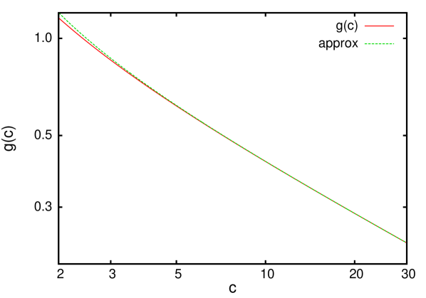
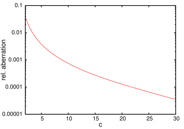
From equation (6) we expect (which has the units of a frequency) to be constant when , and indeed from an asymptotic expansion of equation (2) for large c we obtain and . Fig. 1 shows that satisfies this expectation throughout the entire parameter range of interest. For (), the direct computation of becomes impractical so apart from the advantage of a numerically less costly formula a reasonable approximation must be found. The dashed green line in Fig. 1 demonstrates that for this is achieved to high precision by111Alternatively can be stringently approximated using eq. (8.327) of Gradshteyn & Ryzhik (1980), but our term appears to be the best compromise of simplicity and accuracy throughout the interesting part of the parameter range.
| (17) |
For we adopt the radial dependence
| (18) |
Above we have restricted ourselves to stars with . However, to the extent that the motion in of a star is unaffected by its motion perpendicular to the plane, the distribution we have derived will apply to the population formed by all stars that now lie in the solar cylinder (the region restricted in radius to but unrestricted in ). From our formulae we have that the shape of this velocity distribution is controlled by four parameters: the galactocentric radius of the measurement , the scale-length of the young disc, the local velocity dispersion , and the scale-length on which the velocity dispersion varies. The first two parameters are generally well-known and for fits of the solar neighbourhood can be set to and . The value of is less clear and will be discussed below.
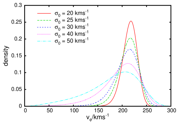
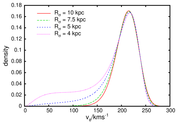
The dependence of on and is shown in Fig. 2. In the upper panel we hold the dispersion scale-length constant at and show the velocity distributions for local dispersion values of . As increases, the distribution becomes wider and the low-velocity tail rises much faster than does the high-velocity tail, corresponding to an increasing asymmetric drift. Simultaneously, the peak slowly shifts to lower velocities. The lower panel shows the velocity distributions for fixed , but different scale-lengths of the velocity dispersion, . Smaller values of imply higher dispersion in the inner regions of the Galaxy and lower dispersion in the outskirts. Thus for small stars from the inner disc can more easily reach the compared to their counterparts with larger so the azimuthal velocity distribution is more skewed and develops a strong low-velocity tail. In the most extreme case, , the model breaks down, as approaches in the inner regions. Notice that as falls, the mode of the velocity distribution shifts to higher even as the tail at high becomes weaker. This effect reflects the fact that stars with large random velocities spread their contributions to the velocity distribution over many radii, while stars with small random velocities localise their contributions. Consequently, when is small, the width in over which stars contribute to narrows strongly as increases, which puts stars with strongly in control of the mode of the local distribution.
3 The velocity distribution as a function of distance from the plane
In the previous section we set to obtain results that are approximately valid for the distribution of stars in regardless of their distance from the plane. In practice we can determine the velocity distributions of the stars that lie in various more-or-less narrow ranges in . We must now consider how these distributions will vary with and differ from the aggregate distribution determined above. In the following we do so using a number of quite crude physical approximations. These approximations give useful physical insight into why the distribution in varies with as it does, but ultimately the value of our final fitting formula does not depend on the correctness of the arguments used to motivate it.
3.1 Weights of different populations as functions of
The key idea is that within the solar cylinder there coexist many populations, one for each value of . Indeed the chemical compositions and ages of stars vary systematically with (see e.g. Luck & Lambert, 2011; Bensby et al., 2011; Schönrich, Binney & Dehnen, 2010, for observations and a short discussion of consequences for studies of kinematics). Moreover, the smaller a population’s value of , the larger will be its mean value of and therefore the larger will be its vertical scale-height at radius ; here is the distance that at radius provides the best fit to the vertical density profile of the population through
| (19) |
Note that with this formula we are not asserting that the real vertical density profile is exponential, but simply identifying the characteristic vertical extent of the population. We now investigate how the vertical extent of the population increases with because the vertical restoring force, which scales like , decreases outwards.
BM11 show that a very good approximation to the vertical dynamics of a population of stars can be obtained by assuming that the vertical action
| (20) |
of the population’s stars is adiabatically invariant as the stars oscillate in radius. We use this adiabatic approximation (aa) to estimate the ratio .
can be evaluated analytically only for a vertical force that is proportional to and to the local surface density of the disc , so we assume these dependencies in order to gain an analytic model – in reality has a much more complex dependence on , which does not yield an analytic expression for . Then the vertical action is
| (21) |
where is a constant and
| (22) |
is the height at which the radical vanishes. In terms of the variable we have
| (23) |
With the aa, it now follows that
| (24) |
The scale-height of the population will scale like , so
| (25) |
Photometry of edge-on spiral galaxies shows that the overall scale-height varies very little with radius (van der Kruit & Searle, 1982). Since the velocity dispersion at radius will be dominated by the population that has , we assume that
| (26) |
is independent of . Hence
| (27) |
For stars that make only small-amplitude vertical oscillations, so . If the amplitude of a star’s oscillations significantly exceeds the local disc scale-height (but is none the less small compared to ), a better approximation is that the disc is razor thin, so and . For amplitudes not small compared to the disc’s scale-length, a yet smaller value of is appropriate. In the fits described below we assumed that decreases with according to
| (28) |
These choices are educated guesses that produce useful results.
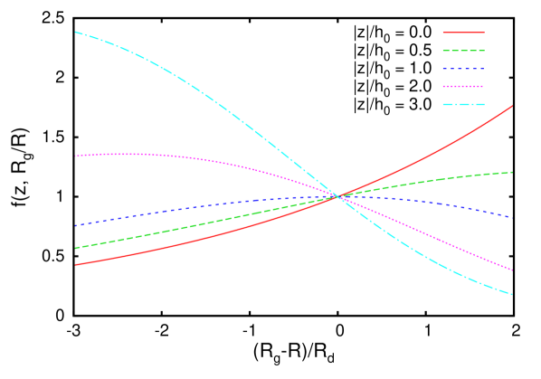
Let the ratio of the contributions to the distribution in at height of the population with guiding-centre radius and the local population be given by the factor . Then from equation (15) the distribution of at altitude above the plane is
| (29) |
where is a new normalisation constant.
By equation (19), the factor will scale as
where in the second step we have used the definition (26). Fig. 3 shows, for five values of , how varies with at . At , is an increasing function of because at large stars typically have small and therefore are more numerous in the plane than in the solar cylinder as a whole. At , by contrast, falls with increasing because high above the plane a sample is richer in stars with small , and therefore large , than is the solar cylinder as a whole. The formula attains a maximum, where the local scale-height of a population equals the altitude. Since by definition gives the enhancement of stars with guiding-centre radius relative to local stars, all lines intersect at (, ) irrespective of the chosen altitude.
3.2 Impact of the AA on the radial motion
The aa predicts that any star’s value of varies as it moves radially. Since the star is moving in a time-independent potential, its total energy is constant. It follows that changes in must be compensated by changes in its energy of motion parallel to the plane. Since is a true invariant, the energy associated with the underlying circular orbit is unchanged, so changes in must be compensated by changes in the radial energy . Hence (3) becomes
| (31) |
where
| (32) |
takes into account the decrease in a star’s vertical energy as it moves outwards: by conservation of energy, this energy must be transferred to the radial motion. One way of thinking about this energy transfer is to imagine that the star moves at constant energy in an effective potential
| (33) |
which might be called the “adiabatic potential” since it is the effective potential for radial motion that follows from adiabatic invariance of the vertical motion. At increases with less rapidly than the standard effective potential , so stars can reach larger radii than they could if were constant. BM11 simulated this effect by simply increasing to .
With the power-law forms of the vertical potential that we introduced above, we can obtain the dependence of on . From equations (22) and (23) we find
| (34) |
so
| (35) |
Our plan is to use to modify our expression (10) for , which has no dependence on and therefore does not specify a value of or . Therefore in equation (35) we now replace by an estimate of the typical vertical energy of the stars that are encountered at with angular momentum . Equation (47) in the Appendix is an expression for in terms of and the vertical component of the gravitational potential.
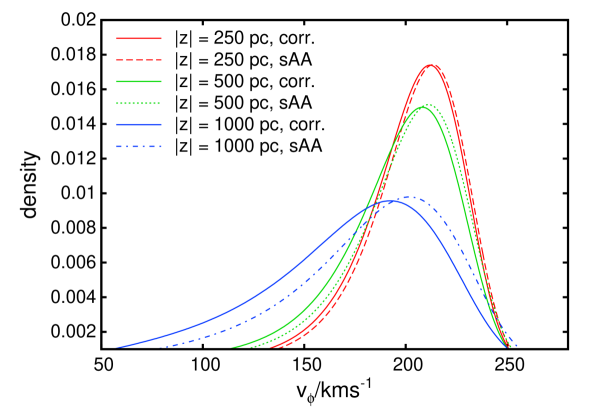
Our next step is essentially to replace by in equation (29) but before we do this we have to recall that the prefactor arose from normalising the radial probability density as given by equation (6). For consistency in this formula we must now replace by , with the consequence that the normalising integral is no longer analytic. Therefore our final formula for the distribution of at a given point in the Galaxy must be written
| (36) | |||||
where is the numerically-determined result of normalising the revised form of [cf eq. (2)], normalises the distribution in and is defined by equation (3.1).
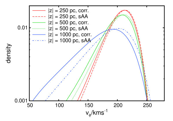
Fig. 4 illustrates the effect that the inclusion of in the effective potential has on by showing for and several values of the velocity distributions predicted with (full curves) and without (dotted curves) . Including moves all velocity distributions to lower , particularly on the left side. The magnitude of the shift increases with because at low , is dominated by orbits with small and therefore small .
Far from the plane () equation (36) breaks down because the physical assumptions on which it depends fail. A problem that must be encountered at some height is that the vertical frequency becomes comparable to the horizontal frequency, so the assumption of adiabatic invariance of fails – the coupling between the horizontal and vertical motions becomes strong and complex. However, BM11 did not encounter problems with the aa below . The failure we encounter here probably arises from equation (47) for , so we below explore the effect of limiting the energy transfer by placing an uper limit on the value of to less than .
3.3 Velocity moments
From the formulae we have in hand we can calculate a variety of moments. Suppose the stellar population of the disc were a superposition of populations that have dfs of the form
| (37) |
where the dependence on is inspired by equation (19). Then since this df is a Gaussian in , we would have . To each value of and therefore we could ascribe a fixed value for , where in general lower are connected to higher . Hence the velocity dispersion of the entire disc could be obtained from the weighted average
| (38) |
Similarly the asymmetric drift would be
| (39) |
From the work of Section 3.2 we know that is not strictly a constant of the motion on account of the transfer of energy between the radial and vertical motions, so these formulae are only approximate. We shall see that they are nevertheless useful.
The df (37) is also a Gaussian in so naively we have for the population formed by stars of a given value of . However, when calculating for the entire disc it is essential to bear in mind the radial variation of implied by adiabatic invariance of (eq. 34). In effect this variation of causes to vary with radius even at fixed . Hence an approximate expression for the vertical velocity dispersion of the entire disc is
| (40) |
4 Applications
4.1 Comparison with torus models
To evaluate the performance of the above equations we fit the velocity distributions of the torus model of BM11. The df of this model is
| (41) |
where
| (42) |
Here is the circular frequency for angular momentum , is the radial epicycle frequency and is its vertical counterpart and is given by equation (8). The factor in equation (42) is there to effectively eliminate stars on counter-rotating orbits and the value of is unimportant provided it is small compared to the angular momentum of the Sun. In equations (41) and (42) the functions and control the vertical and radial velocity dispersions. The observed insensitivity to radius of the scale-heights of extragalactic discs motivates the choices
| (43) |
where and and are approximately equal to the radial and vertical velocity dispersions at the Sun. BM11 take the df of the entire disc to be the sum of a df of the form (41) for the thin disc, and a similar df for the thick disc, the normalisations being chosen so that at the Sun the surface density of thick-disc stars is 23 per cent of the total stellar surface density. Table 1 lists the parameters of each component of the df.
| Disc | ||||
|---|---|---|---|---|
| Thin | 2.4 | 27 | 20 | 10 |
| Thick | 2.5 | 48 | 44 | 10 |
| Component | ||||
|---|---|---|---|---|
| Thin | 36.42 | 2.4 | 0.36 | 0 |
| Thick | 4.05 | 2.4 | 1 | 0 |
| Gas | 8.36 | 4.8 | 0.04 | 4 |
| Component | ||||||
|---|---|---|---|---|---|---|
| Bulge | 0.7561 | 0.6 | 1.8 | 1.8 | 1 | 1.9 |
| Halo | 1.263 | 0.8 | 2.207 | 1.09 | 1000 |
| — | ||||||
BM11 took the gravitational potential to be that of Model 2 in Dehnen & Binney (1998) modified to have thin- and thick-disc scale-heights of and (Table 2). In this model the disc contributes 60 per cent of the gravitational force on the Sun, with dark matter contributing most of the remaining force.
4.1.1 Distribution in
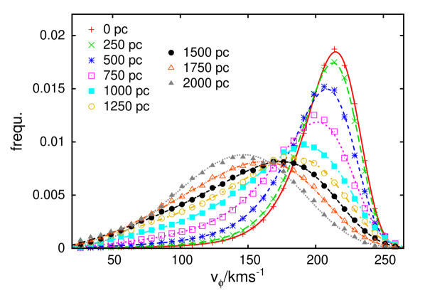
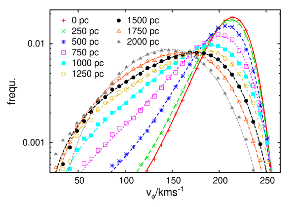
The points in Fig. 5 show the distributions of the BM11 model at and heights up to , while the curves show the fits to these points that we obtain from equation (36) when we approximate with . We take from equation (28) and at each location we fit the given distribution independently by adjusting the parameters , and . Table 3 gives the parameter values obtained from the fits and also the radial velocity dispersions that the fits yield through equation (38) and the true radial velocity dispersion within the model. Notice that the parameter rises from at the plane to at and that these values coincide with the values of the corresponding parameters in the dfs of the thin and thick discs, respectively. Fig. 6 and Table 4 show the fits obtained to the same data when in equation (36) is evaluated from equation (33) with replaced by from equation (47).
In both Figs. 5 and 6 the quality of the fits is excellent, so the inclusion of improves the optimum fit only marginally. However, inclusion of does change the optimum value of significantly and in the sense of bringing it closer to the true scale-height of the model disc, which increases from small values very close to the plane, where the gas disc dominates the gravitational potential, through at , where the thin disc accounts for the majority of stars, to at large heights, where the thick disc is dominant. Note that far from the plane the dominant population’s scale-height is significantly smaller than the locally measured scale-height of the disc because the population is dominated by stars with , which by equation (25) have . Even so, when is omitted, the fitted values of are unexpectedly small. Including increases at all heights, while limiting the values of employed to less than yields intermediate values of , which are not far from constant as we would wish. The reason adding to the effective potential increases is that increases the contribution to the velocity distribution at of stars with small values of and therefore and thus reduces the need to suppress the contribution of the population with , which dominates the peak of the distribution, relative to the stars that form the prominent left wing of the distribution. The other improvement effected by including is to lower slightly and thus bring it closer to its true value at high altitudes. When there is no upper limit on the values of used in the calculation of , this lowering of becomes excessive above because at such altitudes the vertical energy becomes comparable to the radial energy.
Irrespective of whether is used, the scale-length exhibits a continuous rise in the fits, moving away from the value of the corresponding parameter of the torus model. comes closer to the lower is chosen at higher altitudes.


4.1.2 Distributions in
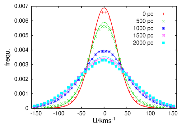
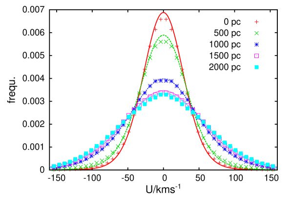
As we remarked in Section 3.3, the df (37) is such that stars of given have a Gaussian distribution in . Consequently, the distribution in of all stars found at a given distance from the plane should in this picture be a weighted sum of Gaussian distributions with the weights implicit in equation (38). Fig. 7 compares this prediction (lines) at several altitudes with the corresponding distributions from the torus models (data points). The overall agreement between the data points and the predictions of the formula is remarkable when one bears in mind that the curves have not been obtained by fitting to the data points. At low altitudes (red and green) the formula predicts a distribution that is slightly too sharply peaked and deficient in the wings. Around from the plane the fit is near perfect. The agreement between the curve for and the data points at is much better in the lower panel than the upper panel, vindicating the use of the correction provided by .
4.2 Application to the Geneva-Copenhagen Survey
We have fitted the full formula (36) at an altitude of to the velocity distribution of the Geneva-Copenhagen Survey (GCS) of F and G stars (Nordström et al., 2004; Holmberg, Nordström & Andersen, 2009). As sample we selected the full objects that have measured space velocities. We adopted and assumed that the Sun’s velocity with respect to the Local Standard of Rest is (Schönrich, Binney & Dehnen, 2010), so was added to the published heliocentric velocities. Given that the sample lies near to the mid-plane, where would apply, we adopted , and we also set the local scale-height to : when and are allowed to vary when fitting to the data, they prove to be strongly correlated in the sense that low values of enhance the contribution of populations with smaller and thus favour larger values of for balance. However, the differences between the residuals of the various best fits are not statistically significant.
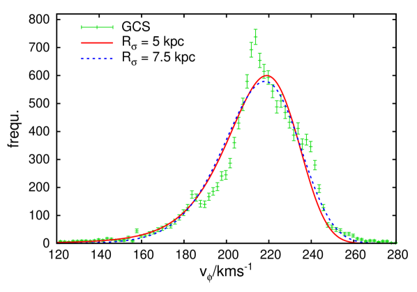
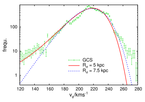
Fig. 8 shows two typical fits performed on the region , which demonstrate how nicely and naturally the formula reproduces the non-Gaussianity of the azimuthal velocity distribution. The fits are for scale-lengths (blue dashed line) and (red solid line). The shorter scale-length provides the better fit at low and the worse fit to the high-velocity tail. The shorter length scale also yields the smaller value of the velocity-dispersion parameter, versus . In the plane the core of the velocity distribution is dominated by the youngest part of the thin disc, while the wings of the distribution will be dominated by the thick disc, and as we proceed from the core to the wings of the distribution stars of ever increasing age will grow in importance. Hence the true distribution in reflects the entire star-formation history of the Galaxy and we cannot expect to obtain a perfect fit to it by adjusting a single velocity-dispersion parameter, . Moreover, the statistics of the GCS catalogue to some extent reflect the complex selection biases involved in the catalogue’s formation, and we have made no attempt to replicate these biases. Neglect of these complexities is presumably why our fit is less good than that obtained by Schönrich, Binney & Dehnen (2010). The presence of kinematically hotter objects is confirmed by the estimated value for drifting to higher values when we expand the velocity interval on which we perform the fits. A couple of thin-disc scale-heights above the plane the population will be more homogeneous, being dominated by the thick disc, and it should be possible to obtain better fits by adjusting .
Interestingly, on testing for a systematic shift in the formula recovered to the expected local standard of rest both from the GCS data and from the velocity distributions of the torus models at low altitudes. At higher altitudes the performance deteriorates due to the higher uncertainties. We found that for local stars does not play a significant role, although it gives a bias of order . In a forthcoming re-determination of the local standard of rest we will take this effect into account.
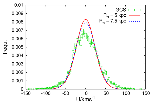
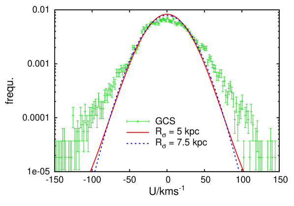
Fig. 9 compares the GCS data with the distributions that follow from the fits to . It is clear that the formula under-estimates the width of the distribution. In Section 4.1.2 we found that in the case of the torus model at small , the fitted distribution was somewhat narrower than the true one even though the distribution was very closely fitted. Correspondingly, in the case of the GCS data, the failure of the fit to the to adequately populate populate the wings of the distribution is mirrored in the fit to the distribution in Fig. 9 being least satisfactory in the wings.
5 Conclusions
The distribution of azimuthal velocities in the disc of a galaxy like ours is very skew and varies systematically with distance from the plane. Naturally one wants to be able to quantify such a distribution in an effective way. The traditional approach of fitting it with a superposition of Gaussians (e.g. Bensby et al., 2003; Ivezić et al., 2008; McConnachie et al., 2006) is unsatisfactory, both because there is no physical reasoning behind the use of a Gaussian when the distribution is not dominated by measurement error, and because when a superposition of Gaussians is used, the parameters of the fit are neither unique nor physically informative.
Our formula is based on the approximation that the vertical actions of stars are invariant as stars oscillate radially. We have refined this approximation by considering anew the impact that vertical motion has on the radial oscillations, which BM11 found to be a significant effect. Our treatment of this effect, being based on overall energy conservation, is conceptually much sounder than that of BM11 and promises to play a valuable role in the interpretation of stellar velocities with rigorous dynamical models. However, we find that the power of our formula is only marginally improved by our more rigorous treatment of how vertical motion affects the radial oscillations.
Ultimately, our formula is just a fitting formula rather than a dynamical theory, even though we have derived it from dynamical considerations. Something the derivation highlights is how closely the horizontal and vertical motions of stars are intertwined, notwithstanding the adiabatic invariance of actions. Because both the vertical and horizontal random velocities of stars increase with age, as one moves away from the plane the mix of stars one sees fundamentally changes in the sense of increasing age and decreasing radius of birth. The cleanest way to model this phenomenon is by means of a df like those presented by Binney (2010), but a couple of computationally challenging steps are required to extract observationally testable velocity distribution such as from a df: first a connection has to be established between ordinary phase-space coordinates and the isolating integrals upon which the df depends, and then one has to marginalise over two velocities. Evaluation of our formula is trivial by comparison.
Our derivation makes it plain that no population of stars can simultaneously have scale-height and velocity dispersion that are both independent of radius: the sub-population formed by stars that have a narrow range of angular momenta must inevitably increase in scale-height and decrease in vertical velocity dispersion with increasing , and if stars of larger angular momenta are added in to hold constant the scale-height, they will have to have an even smaller vertical velocity dispersion, so the vertical dispersion of the entire population will decline steeply outwards. Given this situation, it is unwise to seek to define the thick disc in terms of a given scale-height and velocity dispersion, as some recent papers have done.
We validated our fitting formula by using it to fit the distributions of components at several distances from the plane in a model with a well-defined df that included both thin and thick discs. Excellent fits were obtained. The values of the fitting parameters varied slightly with the level of sophistication of the model employed, but were broadly in agreement with the values we would expect given the underlying df, especially when the most sophisticated approximations were used. This exercise implies that physical significance can be attached to the values of parameters derived from fits to real data. Each fit to a distribution implies a model of the corresponding distribution. In our tests these models turned out to be very useful although showing a slight tendency to be too narrow at small .
We fitted the formula to the velocities of GCS stars and obtained good but not perfect fits for plausible values of the parameters. The blemishes in these fits will arise from three causes: (i) the well known presence of pronounced clumping of stars in the plane (Dehnen, 1998), (ii) the need to model subtle selection effects in the GCS sample, and (iii) our formula is derived from an isothermal df and must encounter difficulty fitting data drawn from a system that is a superposition of systems with very disparate dynamical temperatures. Hence in part the difficulties encountered in fitting the GCS data may reflect the importance at the extremes of the distribution of the thick disc and/or stellar halo. With a larger body of data, or data taken further from the plane, it might be profitable to fit the data to a sum of two or more instances of our formula. Our fit to the components yields a model of the components that is rather too narrow, in agreement with our work with the model based on a df.
Our formula could be used to fit the line-of-sight velocity distributions (LOSVDs) of galaxies in which individual stars are not resolved (e.g. Bacon et al., 2001). Since our formula has been derived on the assumption that the circular speed is independent of radius, it might fail to produce a satisfactory fit to the velocity distribution of stars in a galaxy with a distinctly non-flat rotation curve. The physical basis of our formula breaks down at distances from the plane of order , so failure to fit data for stars at higher altitudes might have no physical significance.
We derived our formula by adapting to the three-dimensional world the planar df of Shu (1969). It would be interesting to adapt in a similar way the planar df of Dehnen (1999), which Dehnen has argued is in certain respects superior to the Shu df. Unfortunately, the adaptation of a planar df is a non-trivial exercise on account of the intertwining of the radial and vertical motions mentioned above. Therefore in this paper we have confined ourselves to the Shu df, which proves to provide a very useful point of departure.
Data for stars that lie at significant distances from the plane are now becoming available (Ivezić et al., 2008; Siebert et al., 2011). The measured space velocities of such stars contain significant errors arising from a combination of errors in proper-motion and distance. It is essential to take proper account of these errors when inferring the true kinematics of the underlying populations. Our formula provides the natural way to do this: one fits the data to the result of folding the formula with appropriate distance and proper-motion errors. Schönrich, Asplund & Casagrande (2011) use this methodology to extract in an elegant way the information contained within the measured distribution of azimuthal velocities of stars that have quite large random velocities. We will shortly present similar analyses of samples that include a higher proportion of disc stars.
Acknowledgements
It is a pleasure to thank Andreas Just for detailed reading of the paper and many very valuable comments. We thank Walter Dehnen for helpful comments on a draft and Paul McMillan for the compilation and discussion of the torus model data. R.S. acknowledges financial and material support from Max-Planck-Gesellschaft. J.B. acknowledges the support of STFC and Merton College, Oxford.
References
- Aumer & Binney (2009) Aumer M., Binney J., 2009, MNRAS, 397, 1286
- Bacon et al. (2001) Bacon R. et al., 2001, MNRAS, 326, 23
- Bensby et al. (2003) Bensby T., Feltzing S., Lundström I., 2003, A&A, 410, 527
- Bensby et al. (2011) Bensby T., Alves-Brito A., Oey M.S., Yong D., Meléndez J., 2011, ApJ, 735, 46
- Binney (2010) Binney J., 2010, MNRAS, 401, 2318
- Binney and McMillan (2011) Binney J., McMillan P., 2011, MNRAS, 413, 1889 (BM11)
- Binney and Tremaine (2008) Binney J., Tremaine S., 2008, Galactic Dynamics, 2nd ed., (Princeton: PUP)
- McConnachie et al. (2006) McConnachie A.W., Chapman S.C., Ibata R.A., Ferguson A.M.N., Irwin M.J., Lewis G.F., Tanvir N.R., Martin N., 2006, ApJL, 647, 25
- Dehnen (1998) Dehnen W., 1998, AJ, 115, 2384
- Dehnen & Binney (1998) Dehnen W., Binney J., 1998, MNRAS, 294, 429
- Dehnen (1999) Dehnen W., 1999, AJ, 118, 1201
- de Grijs, Peletier & van der Kruit (1997) de Grijs R., Peletier R.F., van der Kruit P.C., 1997, A&A, 327, 966
- Gradshteyn & Ryzhik (1980) Gradsteyn I.S., Ryzhik J.M., Table of Integrals, Series, and Products, 4th ed., (London: AP)
- Halliday et al. (2006) Halliday C. et al., 2006, MNRAS, 369, 97
- Holmberg, Nordström & Andersen (2009) Holmberg J., Nordström B., Andersen J., A&A, 501, 941
- Ivezić et al. (2008) Ivezić Ž. et al., 2008, ApJ, 684, 287
- Just & Jahreiß (2010) Just A., Jahreiß H., 2010, MNRAS, 402, 461
- Luck & Lambert (2011) Luck R.E., Lambert D.L., 2011, arXiv:1108.1947v1
- Nordström et al. (2004) Nordström B. et al., 2004, A&A, 418, 989
- Schönrich & Binney (2009) Schönrich R., Binney J., 2009, MNRAS, 396, 203
- Schönrich, Asplund & Casagrande (2011) Schönrich R., Asplund M., Casagrande L., 2011, MNRAS, 415, 3807
- Schönrich, Binney & Dehnen (2010) Schönrich R., Binney J., Dehnen W., 2010, MNRAS, 403, 1829
- Siebert et al. (2011) Siebert A. et al., 2011, AJ, 141, 187
- Shu (1969) Shu F.H., 1969, ApJ, 158, 505
- Steinmetz et al. (2005) Steinmetz M. et al., 2006, AJ, 132, 1645
- Strömberg (1927) Strömberg G., 1927, 65, 238
- van der Kruit & Searle (1982) van der Kruit P.C., Searle L., 1982, A&A, 110, 61
- Yanny et al. (2009) Yanny B. et al., 2009, ApJ, 137, 4377
- York et al. (2000) York, D. G., et al. 2000, AJ, 120, 1579
Appendix: estimating the typical vertical energy
In this appendix we estimate the typical value of the vertical energy of the stars that we encounter with specified angular momentum at a given location . Let be the vertical velocity dispersion at . then
| (44) |
Regarding , we have that to an excellent approximation the vertical Jeans equation reads (Binney and Tremaine, 2008, eq. 4.271)
| (45) |
Neglecting the derivative of relative to that of this yields
| (46) |
where is the local scale-height of the population. As we saw from equation (27) the local scale-height decreases towards lower guiding centre radii, if we assume all populations to have at their guiding centre radius a constant scale-height. Hence finally we adopt:
| (47) |
Equation (47) involves the potential and its derivative at altitude . We obtain these from a simple mass model with a razor thin gas layer that at the solar radius has surface density and three exponential stellar components. In each such component the mass per unit surface area within distance of the plane is
| (48) |
The three components represent the thin disc, the thick disc and the halo with parameters
| (49) |
and
| (50) |
The halo contribution was chosen to match the local vertical potential from the adopted Dehnen potential, which was used for the torus models to which we compare our formalism – the modifications required for a different radius or disc mass are simple. We approximate the contribution to the potential from the th component by assuming that the component is an infinite plane-parallel sheet. Then
| (51) |