External field effect on quantum features of radiation emitted by a QW in a microcavity

Abstract

We consider a semiconductor quantum well in a microcavity driven by coherent light and coupled to a squeezed vacuum reservoir. By systematically solving the pertinent quantum Langevin equations in the strong coupling and low excitation regimes, we study the effect of exciton-photon detuning, external coherent light, and the squeezed vacuum reservoir on vacuum Rabi splitting and on quantum statistical properties of the light emitted by the quantum well. We show that the exciton-photon detuning leads to a shift in polariton resonance frequencies and a decrease in fluorescence intensity. We also show that the fluorescent light exhibits quadrature squeezing which predominately depends on the exciton-photon detuning and the degree of the squeezing of the input field.

I Introduction

Study of radiation-matter interaction, in two level quantum mechanical systems have lead to several fascinating phenomena like the Autler-Townes doublet Aut55 , vacuum Rabi splitting Aga84 ; Tho92 ; Khi06 , antibunching and squeezing Gar86 ; Car87 ; Vya92 . In particular, interaction of two-level atoms in a cavity with a coherent source of light and coupled to a squeezed vacuum has been extensively studied Aga89 ; Par90 ; Cir91 ; Rice96 ; Ge095 ; Smy96 ; Cle20 ; Str05 ; Set08 . Currently there is renewed interest in such studies from the context of semiconductor systems like quantum dots (QDs) and wells (QWs) Baa04 ; Qua05 ; Hic108 ; Hic208 ; Set10 given their potential application in opto-electronic devices Shi07 . In this regard, intersubband excitonic transitions which have similarities to two level atomic system has been primarily exploited. However, it is important to understand that the quantum nature of fluorescent light emitted by excitons in QWs embedded inside a microcavity somewhat differs to that of atomic cavity QED predictions. For example, unlike antibunching observed in atoms embedded in a cavity a QW exhibits bunching effects in the fluorescent spectrum of the emitted radiation Vya20 ; Ere03 . Further in the strong coupling regime, for a resonant microcavity-QW interaction, exciton-photon mode splitting and oscillatory excitonic emission has been demonstrated Wei92 ; Pau95 ; Jac95 . Recently effect of a non-resonant strong drive on the Intersubband excitonic transition has been investigated and observation of Autler Townes doublets were reported Dyn05 ; Car05 ; Wag2010 . In light of these new results an eminent question of interest is thus, how does the quantum nature of radiation emitted from a QW in a microcavity get effected in presence of a squeezed vacuum environment and non-resonant drive? We investigate this in the current paper.

We explore the interaction between an external field and a QW placed in a microcavity coupled to a squeezed vacuum reservoir. Our analysis is restricted to the weak excitation regime where the density of excitons is small. This allows us to neglect any exciton-exciton interaction thereby simplifying our problem considerably and yet preserving the physical insight. We further assume the cavity-exciton interaction to be strong, which brings in interesting features. Note that we consider the external field to be in resonance with the cavity mode throughout the paper. We analyze the effect of exciton-photon detuning, external coherent light, and the squeezed reservoir on the quantum statistical properties and polariton resonances in the strong coupling and low excitation regimes. The effect of the coherent light on the behavior of the dynamical evolution of the intensity fluorescent light is remarkably different to that of the squeezed vacuum reservoir due to the nature of photons generated by the two systems. This is due to the distinct nature of the photons generated by the coherent and squeezed inputs. This effect is manifested on the intensity of the fluorescent light. Both sources lead to excitation of two or more excitons in the quantum well creating a probability for emission of two or more photons simultaneously. As a result of this, the photons tend to propagate in bunches other than at random. Moreover, the fluorescent light emitted by exciton in the quantum well exhibits nonclassical property namely, quadrature squeezing.

II Model and Quantum Langevin equations

We consider a semiconductor quantum well (QW) in a cavity driven by external coherent light and coupled to a single mode squeezed vacuum reservoir. The scheme is outlined in Fig. 1. In this work, we are restricted to a linear regime in which the density of excitons is small so that exciton-exciton scattering can be ignored. We assume that the driving laser is at resonance with the cavity mode while the exciton transition frequency is off resonant with the cavity mode by an amount $\Delta=\omega_{0}-\omega_{c}$ with $\omega_{0}$ and $\omega_{c}$ being the exciton and cavity mode frequencies. The interaction of the cavity mode with the resonant pump field and the exciton is described, in the rotating wave and dipole approximations, by the Hamiltonian

$$H=\Delta b^{\dagger}b+i\varepsilon(a^{\dagger}-a)+i\text{g}(a^{\dagger}b-ab^{\dagger})+H_{\text{loss}},$$ (1)

where $a$ and $b$, are the annihilation operators for the cavity and exciton modes satisfying the commutation relation $[a,a^{\dagger}]=[b,b^{\dagger}]=1$ respectively; g is the photon-exciton coupling constant; $\varepsilon$, assumed to be real and constant, is proportional to the amplitude of the pump field, and $H_{\text{loss}}$ is the Hamiltonian that describes the interaction of the exciton with the vacuum reservoir and also the interaction of the cavity mode with the squeezed vacuum reservoir.

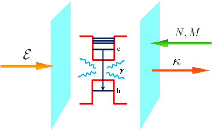
Figure 1: Schematic representation of a quantum well (QW) in a driven cavity coupled to a squeezed vacuum reservoir.

The quantum Langevin equations, taking into account the dissipation processes, can be written as

$$\frac{da}{dt}=-\frac{\kappa}{2}a+\text{g}b+\varepsilon+F(t),$$ (2)

$$\frac{db}{dt}=-(\frac{\gamma}{2}+i\Delta)b-\text{g}a+G(t),$$ (3)

where $\kappa$ and $\gamma$ are cavity mode decay rate via the port mirror and spontaneous emission decay rate for the exciton, respectively; $F=\sqrt{\kappa}F_{\text{in}}$ and $G=\sqrt{\gamma}G_{\text{in}}$ with $F_{\text{in}}$ and $G_{\text{in}}$ being the Langevin noise operators for the cavity and exciton modes, respectively. Both noise operators have zero mean, i.e., $\langle F_{\text{in}}\rangle=\langle G_{\text{in}}\rangle=0$. For a cavity mode coupled to a squeezed vacuum reservoir, the noise operator $F_{\text{in}}(t)$ satisfies the following correlations:

$$\left\langle F_{\text{in}}(t)F_{\text{in}}^{\dagger}(t^{\prime})\right\rangle=(N+1)\delta(t-t^{\prime}),$$ (4)

$$\left\langle F_{\text{in}}^{\dagger}(t)F_{\text{in}}(t^{\prime})\right\rangle=N\delta(t-t^{\prime}),$$ (5)

$$\left\langle F_{\text{in}}(t)F_{\text{in}}(t^{\prime})\right\rangle=\left\langle F_{\text{in}}^{\dagger}(t)F_{\text{in}}^{\dagger}(t^{\prime})\right\rangle=M\delta(t-t^{\prime}),$$ (6)

where $N=\sinh^{2}r$ and $M=\sinh r\cosh r$ with $r$ being the squeeze parameter characterize the mean photon number and the phase correlations of the squeezed vacuum reservoir, respectively. Further, the exciton noise operator $G_{\text{in}}$ satisfies the following correlations:

$$\left\langle G_{\text{in}}(t)G_{\text{in}}^{\dagger}(t^{\prime})\right\rangle=\delta(t-t^{\prime}),$$ (7)

$$\left\langle G_{\text{in}}^{\dagger}(t)G_{\text{in}}(t^{\prime})\right\rangle=\left\langle G_{\text{in}}(t)G_{\text{in}}(t^{\prime})\right\rangle=\left\langle G_{\text{in}}^{\dagger}(t)G_{\text{in}}^{\dagger}(t^{\prime})\right\rangle=0.$$ (8)

Following the method outlined in Set10 , we obtain the solution of the quantum Langevin equations (2) and (3) in the strong coupling regime ($g\gg\gamma,\kappa$) to be

$$a(t) =\eta_{1}(t)\varepsilon+\eta_{+}(t)a(0)+\eta_{3}(t)b(0)$$

$$+\int_{0}^{t}dt^{\prime}\eta_{+}(t-t^{\prime})F(t^{\prime})+\int_{0}^{t}dt^{\prime}\eta_{3}(t-t^{\prime})G(t^{\prime}),$$ (9)

$$b(t) =\eta_{-}(t)b(0)-\eta_{4}(t)\varepsilon-\eta_{3}(t)a(0)$$

$$-\int_{0}^{t}dt^{\prime}\eta_{3}(t-t^{\prime})F(t^{\prime})+\int_{0}^{t}dt^{\prime}\eta_{-}(t-t^{\prime})G(t^{\prime}),$$ (10)

where

$$\eta_{1}(t)=\frac{1}{\mu}\sin\mu t~{}e^{-(\Gamma+i\Delta/2)t},$$ (11)

$$\eta_{\pm}(t)=\frac{1}{2\mu}\left[2\mu\cos\mu t\pm i\Delta\sin\mu t\right]e^{-(\Gamma+i\Delta/2)t},$$ (12)

$$\eta_{3}(t)=\frac{g}{\mu}\sin\mu te^{-(\Gamma+i\Delta/2)t},$$ (13)

$$\eta_{4}(t)=\frac{1}{g}-\frac{1}{g}\left[\cos(\mu t)+\frac{i\Delta}{2\mu}\sin\mu t)\right]e^{-(\Gamma+i\Delta/2)t},$$ (14)

where $\Gamma=(\kappa+\gamma)/4$ and $\mu=\sqrt{g^{2}+\Delta^{2}/4}$. Using these solutions we study the dynamical behavior of intensity, power spectrum, second-order correlation function, and quadrature variance for the fluorescent light emitted by the quantum well in the following sections.

III Intensity of fluorescent light

In this section we analyze the properties of the fluorescent light emitted by excitons in the quantum well. In particular, we study the effect of the external driving field, exciton-photon detuning, and the squeezed vacuum reservoir. Note that the intensity of the fluorescent light is proportional to the mean number of excitons. To this end, the intensity of the fluorescent light can be expressed in terms of the solutions of the Langevin equations as

$$\langle b^{\dagger}b\rangle=\varepsilon^{2}|\eta_{4}(t)|^{2}+|\eta_{-}(t)|^{2}+\kappa N\int_{0}^{t}|\eta_{3}(t-t^{\prime})|^{2}dt^{\prime}.$$ (15)

Here we have assumed the cavity mode is initially in vacuum state [$\langle a^{\dagger}(0)a(0)\rangle=0$] while the quantum well initially contains only one exciton [$\langle b^{\dagger}(0)b(0)\rangle=1$]. In (15) the first term corresponds to the contribution from the external coherent light while the last term is due to the the squeezed vacuum reservoir. It is also easy to see that the intensity is independent of the parameter $M$, which characterizes the phase correlations of the reservoir, implying that the same result could be obtained if the cavity mode is coupled to a thermal reservoir.

Performing the integration using Eqs. (13)-(14), we obtain

$$\langle b^{\dagger}b\rangle =\frac{\varepsilon^{2}}{g^{2}}+\frac{g^{2}\kappa N}{4\Gamma\mu^{2}}+(\lambda_{1}+\kappa N\lambda_{2})e^{-2\Gamma t}$$

$$+\frac{\varepsilon^{2}}{g^{2}}\left(\lambda_{1}e^{-2\Gamma t}-2\lambda_{3}e^{-\Gamma t}\right),$$ (16)

where

$$\lambda_{1}(t)=\frac{\Delta^{2}}{4\mu^{2}}\sin^{2}\mu t+\cos^{2}\mu t,$$ (17)

$$\lambda_{2}(t)=-\frac{g^{2}}{4\mu^{2}}\Big{(}\frac{1}{\Gamma}+\frac{1}{\mu}\sin 2\mu t\Big{)},$$ (18)

$$\lambda_{3}(t)=\cos\mu t\cos(\Delta t/2)+\frac{\Delta}{2\mu}\sin\mu t\sin(\Delta t/2).$$ (19)

We immediately see that the intensity of the fluorescent light reduces in the steady state to

$$\langle b^{\dagger}b\rangle_{ss}=\frac{\varepsilon^{2}}{g^{2}}+\frac{g^{2}\kappa N}{4\Gamma\mu^{2}}.$$ (20)

As expected the steady state intensity is inversely proportional to the decay rate. The higher the decay rate the lower the intensity and vise versa.

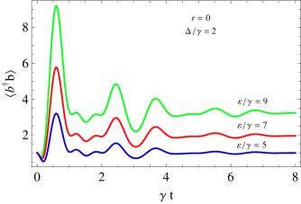
Figure 2: Plots of the fluorescent intensity [Eq. (21)] vs scaled time $\gamma t$ for $\kappa/\gamma=1.2$, $g/\gamma=5$, $\Delta/\gamma=2$, and for different values of $\varepsilon/\gamma$.

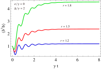
Figure 3: Plots of the fluorescent intensity [Eq. (22)] vs scaled time $\gamma t$ for $\kappa/\gamma=1.2$, $g/\gamma=5$, $\Delta/\gamma=2$, not external driving field ($\varepsilon/\gamma=0$) and for different values of $r$.

In order to clearly see the effect of the external coherent light on the intensity, we set $N=0$ in Eq. (20) and obtain

$$\langle b^{\dagger}b\rangle=\frac{\varepsilon^{2}}{g^{2}}(1+\lambda_{1}e^{-2\Gamma t}-2\lambda_{3}e^{-\Gamma t}).$$ (21)

Figure 2 shows the dependence of the intensity of the fluorescent light on the external coherent field. In general, the intensity increases with the amplitude of the pump field and exhibits non periodic damped oscillations. Although there is a decrease in the mean number of excitons for the initial moment, cavity photons gradually excite one or more excitons in the quantum well leading to enhanced emission of fluorescence. However, the excitation of excitons saturates as time progresses limited by the strength of the applied field. From the steady state intensity, $\varepsilon^{2}/g^{2}$, we easily see that the field strength has to exceed the exciton-photon coupling constant in order to see more than one exciton in the quantum well in the long time limit.

On the other hand, the effect of the squeezed vacuum can be studied by turning off the external driving field. Thus setting $\varepsilon=0$ in Eq. (20), we get

$$\langle b^{\dagger}b\rangle=\frac{g^{2}\kappa N}{4\Gamma\mu^{2}}+(\lambda_{1}+\kappa N\lambda_{2})e^{-2\Gamma t}.$$ (22)

In Fig. 3, we plot the intensity of the light emitted by the exciton [Eq. (22)] as a function of scaled time $\gamma t$ for a given photon-exciton detuning. This figure illustrates the dependence of the intensity on squeezed vacuum reservoir impinging via the partially transmitting mirror. Here also the intensity exhibits damped oscillations at frequency $2\mu=2(g^{2}+\Delta^{2}/4)^{1/2}$ indicating exchange of energy between the excitons and cavity mode. The intensity decreases at the initial moment and gradually increases to steady state values $g^{2}\kappa N/4\Gamma\mu^{2}$. While the intensity increases it shows oscillatory behavior which ultimately disappears for longer times. Unsurprisingly, the intensity increases with the number of photons coming in through the mirror. Comparing Figs. 2 and 3, we note that the intensity has different behavior for the two cases. This can be explained in terms of the nature of photon each source is producing. In the case of coherent light, the photon distribution is Poisson and the photons propagate randomly. This leads to uneven excitation of excitons that results in nonperiodic oscillatory nature of the intensity. In the case of squeezed vacuum source, however, the photons show bunching property and hence can excite two or more excitons at the same time. This in turn implies that depending on the strength of the impinging squeezed vacuum field, there will be one or more excitons in the quantum well.

For the sake of completeness we further consider the effect of detuning on the intensity of the fluorescent light at a given pump field strength and squeezed photons. Figure 4 shows the intensity as a function of scaled time $\gamma t$. When the photon is out of resonance with the exciton frequency there will be less number of excitons in the quantum well and hence the fluorescent intensity decreases. This is clearly shown in Fig. 4.

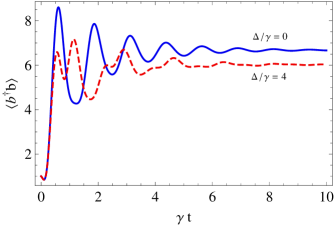
Figure 4: Plots of the fluorescent intensity [Eq. (20)] vs scaled time $\gamma t$ for $\kappa/\gamma=1.2$, $g/\gamma=5$, $r=1.8$, pump amplitude $\varepsilon/\gamma=7$ and for different values of exciton-photon detuning ($\Delta/\gamma$).

IV Power spectrum

The power spectrum of the fluorescent light in the steady state is given by

$$S(\omega)=\frac{1}{\pi}\text{Re}\int_{0}^{\infty}d\tau~{}e^{i(\omega-\omega_{0})\tau}\langle b^{\dagger}(t)b(t+\tau)\rangle_{ss},$$ (23)

where $ss$ stands for steady state. The two time correlation function that appears in the above integrand is found to be

$$\langle b^{\dagger}(t)b(t+\tau)\rangle_{ss} =\frac{\varepsilon^{2}}{g^{2}}+\frac{\kappa Ng^{2}}{4\Gamma\mu^{3}}e^{-(\Gamma+2i\Delta/2)\tau}$$

$$\times(\mu\cos\mu\tau+\Gamma\sin\mu\tau).$$ (24)

Now employing this result in (23) and performing the resulting integration and carrying out the straightforward arithmetic, we obtain

$$S(\omega)=\frac{\varepsilon^{2}}{2\pi g^{2}}\delta(\omega-\omega_{0})+S_{\text{incoh}}(\omega),$$ (25)

where

$$S_{\text{incoh}}(\omega) =\frac{kNg^{2}}{16\pi\mu^{3}}\Big{\{}\frac{\Delta+4\mu-2\omega}{\Gamma^{2}+[\frac{\Delta}{2}+\mu-(\omega-\omega_{0})]^{2}}$$

$$+\frac{-\Delta+4\mu+2\omega}{\Gamma^{2}+[\frac{\Delta}{2}-\mu-(\omega-\omega_{0})]^{2}}\Big{\}}.$$ (26)

We note that the power spectrum has two components: coherent and incoherent parts. The coherent component is represented by the delta function, which indeed corresponds to the coherent light. The incoherent component given by (IV), arises as a result of the squeezed photons coming through the port mirror. From Eq. (IV) it is clear that the spectrum of the incoherent light is composed of two Lorentzians having the same width $\Gamma$ but centered at two different frequencies:$\omega-\omega_{0}=\mu+\Delta/2$ and $\omega-\omega_{0}=\mu-\Delta/2$. We then see that the detuning leads to a shift in the resonance frequency components observed in zero detuning ($\Delta=0)$.

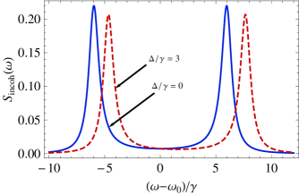
Figure 5: Plots of the incoherent component of the power spectrum [Eq. (IV)] vs scaled frequency $(\omega-\omega_{0})/\gamma$ for $\kappa/\gamma=1.2$, $g/\gamma=6$, squeeze parameter $r=1$, and for different values of detuning, $\Delta/\gamma$.

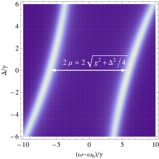
Figure 6: Density plot of the incoherent component of the power spectrum [Eq. (IV)] vs scaled frequency $(\omega-\omega_{0})/\gamma$ and $\Delta/\gamma$ for $\kappa/\gamma=1.2$, $g/\gamma=6$, and for squeeze parameter $r=1$.

Table 1: List of eigenvalues and eigenstates for single and two excitation manifolds. Here $\chi_{\pm}=\sqrt{4g^{2}+(\Delta^{2}\pm 2\mu)^{2}}$.

	Eigenvalues(shifts)	Eigenstates (Exciton polartions)
Single excitation	$\Delta/2+\mu$	$|1\rangle_{+}=[(\Delta+2\mu)|1,0\rangle+2ig|0,1\rangle]/\chi_{+}$
manifold
	$\Delta/2-\mu$	$|1\rangle_{-}=\left[(\Delta+2\mu)|1,0\rangle+2ig|0,1\rangle\right]/\chi_{-}$
Two excitation	$\Delta+2\mu$	$|2\rangle_{+}=[-i\sqrt{2}g|2,0\rangle+(\Delta+2\mu)|1,1\rangle+i\sqrt{2}g|0,2\rangle]/\chi_{+}$
manifold
	$\Delta$	$|2\rangle_{0}=[-i\sqrt{2}g|2,0\rangle+\Delta|1,1\rangle+i\sqrt{2}g|0,2\rangle]/\mu$
	$\Delta-2\mu$	$|2\rangle_{-}=[-i\sqrt{2}g|2,0\rangle+(\Delta-2\mu)|1,1\rangle+i\sqrt{2}g|0,2\rangle]/\chi_{-}$

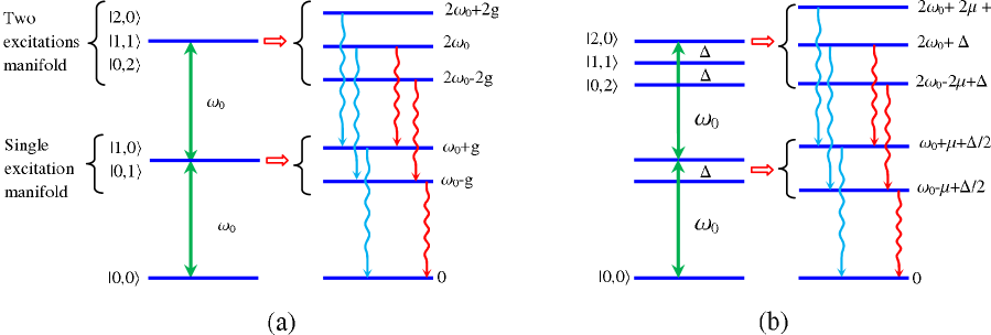
Figure 7: (a) Dressed state energy level diagram for single and two excitation manifolds when the exciton is at resonance with photon. (b) Dressed states energy level diagram when the exciton frequency is detuned by $\Delta$ from that of the photon. We have assumed $\Delta$ to be positive for sake of simplicity. The bare states $|n,m\rangle(n,m=0,1,2)$ represent $n$ numbers of excitons and $m$ numbers of photons. Even though there are 6 possible transitions there are only 2 distinct transition frequencies namely: $\omega-\omega_{0}=\mu+\Delta/2$ and $\omega-\omega_{0}=-\mu+\Delta/2$, where $\mu=\sqrt{g^{2}+\Delta^{2}/4}$.

In Fig. 5 we plot the incoherent component of the power spectrum as a function of scaled time $\gamma t$ for the cavity mode initially in vacuum state and for the quantum well initially containing one exciton. For zero detuning the power spectrum consists of two well resolved peaks centered at $\omega-\omega_{0}=\pm g$. This splitting can be understood from the dressed state energy level diagram (see Fig 7(a)). Note that for the case in which there is only one excitation, there are two possible degenerate bare states: $|1,0\rangle$–one exciton and no photon, and $|0,1\rangle$–one photon no exciton. However, the strong exciton-photon coupling lifts the degeneracy of these two bare states and results in two dressed states (exciton polaritons) $|+\rangle=(|1,0\rangle+i|0,1\rangle)/\sqrt{2}$ and $|-\rangle=(|1,0\rangle-i|0,1\rangle)/\sqrt{2}$ with eigenvalues $g$ and $-g$, respectively. In general, since the exciton-photon system is coupled to the environment, exciton polartions are unstable states. Thus the decay of the exciton and cavity photon leads to exciton polaritons decay, which yields two peaks in the emission spectrum.

It is worth to note that even though we start off with a single exciton in the quantum well, the cavity photons excite two or more excitons in the quantum well. This results in more dressed states in multi excitation manifolds. For example, as shown in Fig. 7(a), for two excitation manifolds there are three dressed states which are equally spaced in energy. This energy separation is the same as the energy separation in one excitation manifold. Out of the six possible transitions, from two excitations to single excitation and then from single to ground state, there are only two distinct frequencies. Therefore, the emission spectrum consists of two peaks. This is different from the atom-photon coupling in which the increase in excitation number increases the number of emission spectrum peaks.

On the other hand, for nonzero detuning case, the emission spectrum has two peaks whose centers are shifted to red (for positive detuning). Here the one excitation bare states ($|1,0\rangle,|0,1\rangle$) are separated by $\Delta$ and the two excitation states ($|2,0\rangle,|1,1\rangle$, and $|0,2\rangle$) as well. The eigenvalues and corresponding eigenstates are given in Table I. The exciton-photon coupling leads to the generation of dressed states (exciton polaritons). The decay of these states to the one excitation and to the ground state gives rise to two emission peaks whose frequencies are different from the zero detuning case as shown in Fig. 7 (b). Further, the density plot for the power spectrum clearly shows that there are indeed two peaks separated by $2\mu=2\sqrt{g^{2}+\Delta^{2}/4}$ as illustrated in Fig. 6.

V Second-order correlation function

In this section we study the second-order correlation function of the light emitted by the quantum well. Second-order correlation function is a measure of the photon correlations between some time t and a later time $t+\tau$. It is also an indicator of a quantum feature that doesn’t have classical analog. Quantum mechanically the second-order correlation function is defined by

$$\text{g}^{(2)}\left(\tau\right)=\frac{\left\langle b^{\dagger}(t)b^{\dagger}(t+\tau)b(t+\tau)b(t)\right\rangle_{ss}}{\left\langle b^{\dagger}(t)b(t)\right\rangle_{ss}^{2}}.$$ (27)

The correlation function that appears in (27) can be obtained using the solution (20) and together with the properties of the Langevin noise forces. Note that as the mean values of the noise forces are zero and the Langevin equations are linear we apply the Gaussian properties of the noise forces. To this end, using Eq. (20), we obtain

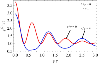
Figure 8: Plot of second-order correlation function versus normalized time $\gamma\tau$ for $g/\gamma=5$, $\kappa/\gamma=1.2$, $\Delta/\gamma=0$, squeezing parameter $r=1$, and for different value of pump amplitude $\varepsilon/\gamma$.

$$\text{g}^{(2)}(\tau)=1 +\frac{1}{\langle b^{\dagger}b\rangle_{ss}^{2}}\Big{[}\frac{\kappa^{2}}{4}\left(4M^{2}A_{3}+N^{2}A_{2}^{2}\right)e^{-2\Gamma\tau}$$

$$+\frac{\kappa\varepsilon^{2}}{g^{2}}\left[MA_{1}+NA_{2}\cos(\Delta\tau/2)\right]e^{-\Gamma\tau}\Big{]},$$ (28)

where

$$A_{1}(\tau) =\frac{2\mu\cos\mu\tau\sin(\Delta\tau/2)-\Delta\cos(\Delta\tau/2)\sin\mu\tau}{4\mu^{2}}$$

$$+\frac{g^{2}\cos\mu\tau[2\Gamma\cos(\Delta t/2)-\Delta\sin(\Delta t/2)]}{\mu^{2}[\Delta^{2}+4\Gamma^{2}]},$$ (29)

$$A_{2}(\tau)=\frac{g^{2}}{2\Gamma\mu^{3}}\left(\mu\cos\mu\tau+\Gamma\sin\mu\tau\right),$$ (30)

$$A_{3}(\tau)=\frac{4\mu^{2}\cos^{2}\mu\tau+\Delta^{2}\sin^{2}\mu\tau+4\Gamma\mu\sin(2\mu\tau)}{16\mu^{2}[\Delta^{2}+4\Gamma^{2}]},$$ (31)

and $\langle b^{\dagger}b\rangle_{ss}$ is given by (20). The term in Eq. (V) represents the second order correlation function for the coherent light. This can easily be seen by setting $N=M=0$. The first term in the square bracket is the contribution to the second-order correlation function from the squeezed vacuum reservoir while the second term describes the interference term between the coherent field and the reservoir. Note that at $\tau\rightarrow\infty$ $\text{g}^{(2)}$ becomes unity as it should be, showing no correlation between the photons.

The dynamical behavior of the second-order correlation function is illustrated in Fig. 8. We see from this figure that the correlation function shows oscillatory behavior with oscillation frequency equal to the photon-exciton coupling constant (g) for zero detuning case and in the absence of the external driving field. However, the frequency of oscillation is reduced by a factor of 1/2 in the presence of external coherent field.

It easy to see that $\text{g}^{(2)}(0)$ is always greater than unity indicating photon bunching. This is in contrary to what has been observed in atomic cavity QED, where the photons show antibunching property Set08 . This is due to the fact that there is a finite time delay between absorbtion and subsequent emission of a photon by the atom. In the case of semiconductor cavity QED, however, the cavity photons can excite two or more excitons at the same time depending on the number of photons in the cavity leading to possible multi photon emission. This is the reason why the photons emitted by excitons are bunched. Indeed, excitation of two or more excitons in the quantum well is shown in Figs. 2-4.

VI Quadrature squeezing

Next we study the squeezing properties of the fluorescent light by evaluating the variances of the quadrature operators. The variances of the quadrature operators for the fluorescent light is given by

$$\Delta b_{\pm}^{2}=1+2\langle b^{\dagger}b\rangle\pm\left[\langle b^{2}\rangle+\langle b^{\dagger 2}\rangle\right]\mp(\langle b^{\dagger}\rangle\pm\langle b\rangle)^{2},$$ (32)

where $b_{+}=(b^{\dagger}+b)$ and $b_{-}=i(b^{\dagger}-b)$. It can be easily seen from this definition that the quadrature operators satisfy the commutation relation $[b_{+},b_{-}]=2i$. It is well known that for the fluorescent light to be squeezed the variances of the quadrature operators should satisfy the condition that either $\Delta b_{+}^{2}<1$ or $\Delta b_{-}^{2}<1$. Using Eq. (II) and the properties of the noise operators we find the variances to be

$$\Delta b_{\pm}^{2} =1+\frac{\kappa Ng^{2}}{2\Gamma\mu^{2}}\pm\frac{2\kappa Mg^{2}\Gamma}{\mu^{2}(\Delta^{2}+4\Gamma^{2})}$$

$$+\Big{[}2\lambda_{1}(t)+2\kappa N\lambda_{2}(t)\pm\kappa M\lambda_{4}\Big{]}e^{-2\Gamma t},$$ (33)

in which $\lambda_{1}$ and $\lambda_{2}$ are same as defined earlier in section (III) and

$$\lambda_{4} =\frac{g^{2}}{\mu^{2}}\Bigg{[}\frac{\Delta\sin(\Delta t/2)-2\Gamma\cos(\Delta t)}{\mu^{2}(\Delta^{2}+4\Gamma^{2})}$$

$$-\frac{\sin[(\Delta-2\mu)t]}{2((\Delta-2\mu))}-\frac{\sin[(\Delta+2\mu)t]}{2((\Delta+2\mu))}\Bigg{]}$$

It is straightforward to see that in the steady state the variances reduce to

$$\Delta b_{+}^{2} =1+\frac{\kappa Ng^{2}}{2\Gamma\mu^{2}}+\frac{2\kappa Mg^{2}\Gamma}{\mu^{2}(\Delta^{2}+4\Gamma^{2})},$$ (34)

$$\Delta b_{-}^{2} =1+\frac{\kappa Ng^{2}}{2\Gamma\mu^{2}}-\frac{2\kappa Mg^{2}\Gamma}{\mu^{2}(\Delta^{2}+4\Gamma^{2})}.$$ (35)

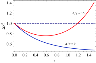
Figure 9: Plots of the steady state quadrature variance [(35)] vs squeeze parameter $r$ for $g/\gamma=5$, $\kappa/\gamma=1.2$, and for the different values of exciton-photon detuning $\Delta/\gamma$ .

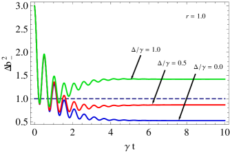
Figure 10: Plots of the quadrature variance [(VI)] vs scaled time $\gamma t$ for $g/\gamma=5$, $\kappa/\gamma=1.2$, squeeze parameter $r=1$ and for the different values of exciton-photon detuning $\Delta/\gamma$.

From the above expressions we find that, in the steady state, the quadrature variances crucially depend on the detuning, the cavity-exciton coupling strength and amount of squeezing provided by the reservoir. Further, it is apparent that if there is any squeezing it can only be present in the $b_{-}$ quadrature. Thus for rest of this section we will only discuss the properties of variance in the $b_{-}$ quadrature. As a special case, we consider that the cavity mode to be at resonance with with the excitonic transition frequency and put $\Delta=0$ in Eq. (35). We then find that

$$\Delta b_{-}^{2}=1-\frac{\kappa}{\kappa+\gamma}(1-e^{-2r})<1.$$ (36)

Equation (36) then suggest that higher squeezing in the reservoir leads to better squeezing of the fluorescent light. In Fig. 9 we confirm this behavior by plotting the steady state $\Delta b_{-}^{2}$ as a function of the squeezing parameter $r$. In addition, from Eq. (36) we see that as $e^{-2r}\rightarrow 0$ quickly with increase in $r$ the maximum possible squeezing achievable in our system is $50\%$ for $\kappa=\gamma$. This is also depicted to be true in Fig. 9.

In presence of detuning $(\Delta\neq 0)$ the behavior of $\Delta b_{-}^{2}$ changes dramatically. We find that for some small detuning $\Delta/\gamma=0.5$ there exist a range of the squeezing parameter $r~{}(0<r<1.3)$ where one can see squeezing of the fluorescent light emitted from the exciton, however for higher values of $r$ it vanishes. This thus implies that in presence of detuning stronger squeezing of the reservoir leads to negative effect on the squeezing of the emitted radiation from the excitons. In Fig. 10, we plot the time evolution of the quadrature variance $\Delta b_{-}^{2}$ (Eq. VI) as a function of the normalized time $\gamma t$ for $r=1$ and different values of detuning. It is seen, in general, that the variance oscillates initially with the amplitude of oscillation gradually damping out at longer time. Eventually, at large enough time the variance becomes flat and approaches to the steady state value. Interestingly, our results show that even though there is no squeezing of the fluorescent light at the initial moment, for small or zero detuning, transient squeezing gradually develops. Moreover, we also find that for weak squeezing of the reservoir, even in presence of small detuning, the initial transient squeezing is sustained and finally leads to a steady state squeezing. This can be understood as a consequence of strong interaction of the quantum well with the squeezed photon entering via the cavity mirror. In case of large detuning the exciton is unable to absorb photons from the squeezed reservoir and thus no squeezing develops in the fluorescence.

VII Conclusion

In this paper we consider a semiconductor quantum well in a cavity driven by external coherent light and coupled to a single mode squeezed vacuum reservoir. We study the photon statistics and nonclassical properties of the light emitted by the quantum well in the presence of exciton-photon detuning in the strong coupling regime. The effects of coherent light and the squeezed vacuum reservoir on the intensity of the fluorescence are quite different. The former leads to a transient peak intensity which eventually decreases to a considerably smaller steady state value. In contrast, the latter, however, gives rise to a gradual increase in the intensity and leads to maximum intensity at steady state. This difference is attributed to the nature of photons that the two sources produce. As a signature of strong coupling between the excitons in the quantum well and cavity photons the emission spectrum consists of two peaks corresponding to the two eigenenergies of the dressed states. Further, we find that the fluorescence exhibit nonclassical feature–quadrature squeezing–as a result of strong interaction of the excitons with the squeezed photons entering via the cavity mirror. In view of recent successful experiments on Autler-Townes effect in GaAs/AlGaAs Wag2010 and gain without inversion in semiconductor nanostructures Fro2006 , the quantum statistical properties of the fluorescence emitted by the quantum well can be tested experimentally.

- (1) S. H. Autler and C. H. Townes, Phys. Rev. 100, 703 (1955).
- (2) G. S. Agarwal, Phys. Rev. Lett. 53, 1732 (1984)
- (3) R. J. Thompson, G. Rempe, and H. J. Kimble, Phys. Rev. Lett. 68, 1132 (1992).
- (4) For a review on vacuum Rabi splitting in semiconductors see G. Khitrova et. al., Nature 2, 81 (2006).
- (5) C. W. Gardiner, Phys. Rev. Lett. 56 , 1917 (1986).
- (6) H. J. Carmichael, A. S. Lane, and D. F. Walls, Phys. Rev. Lett. 58, 2539 (1987) ; J. Mod. Opt. 34, 821 (1987).
- (7) R. Vyas, and S. Singh, Phys. Rev. A 45, 8095 (1992).
- (8) N. Ph. Georgiades, E. S. Polzik, K. Edamatsu, H. J. Kimble, and A. S. Parkins, Phys. Rev. Lett. 75, 3426 (1995).
- (9) G. S. Agarwal, Phys. Rev. A. 40, 4138 (1989).
- (10) A. S. Parkins, Phys. Rev. A. 42, 4352 (1990).
- (11) J. I. Cirac, and L. L. Sanchez-Soto, Phys. Rev. A 44, 1948 (1991).
- (12) P. R. Rice, and C. A. Baird, Phys. Rev. A. 53, 3633 (1996).
- (13) W. S. Smyth, and S. Swain, Phys. Rev. A, 53, 2846 (1996).
- (14) J. P. Clemens, P.R. Rice, P. K. Rungta, and R. J. Brecha, Phys. Rev. A 62, 033802 (2000).
- (15) C. E. Strimbu, J. Leach, and P. R. Rice, Phys. Rev. A 71, 013807 (2005).
- (16) E. Alebachew and K. Fessah, Opt. Comm. 271, 154 (2007);E. Alebachew, J. Mod. Opt 55, 1159 (2008).
- (17) A. Baas, J. Ph. Karr, H. Eleuch, and E. Giacobino, Phys. Rev. A 69, 023809 (2004).
- (18) A. Quattropani and P. Schwendimann, Phys. Status. Solidi 242, 2302 (2005).
- (19) H. Eleuch, J. Phys. B 41, 055502 (2008).
- (20) H. Eleuch, Eur. Phys. J. D 49, 391 (2008); 48, 139 (2008).
- (21) E. A. Sete and H. Eleuch, Phys. Rev. A 82, 043810 (2010).
- (22) A. J. Shields, Nature Photonics 1, 215 (2007).
- (23) R. Vyas, and S. Singh, J. Opt. Soc. Am. B 17, 634 (2000).
- (24) D. Erenso, R. Vyas, and S. Singh, Phys. Rev. A 67, 013818 (2003).
- (25) C. Weisbuch, M. Nishioka, A. Ishikawa, and Y. Arakawa, Phys. Rev. Lett. 69, 3314 (1992).
- (26) S. Pau, G. Bjork, J. Jacobson, H. Cao, and Y. Yamamoto, Phys. Rev. B 51, 14437 (1995); H. Cao et. al. Appl. Phys. Lett. 66, 1107 (1995).
- (27) J. Jacobson, S. Pau, H. Cao, G. Bjork, and Y. Yamamoto, Phys. Rev. A 51, 2542 (1995)
- (28) J. F. Dynes, M.D. Frogley, M. Beck, J. Faist, and C.C. Phillips, Phys. Rev. Lett. 94, 157403 (2005).
- (29) S. G. Carter et. al. Science 310, 651 (2005)
- (30) M. Wagner et. al. Phys. Rev. Lett. 105, 167401 (2010).
- (31) M.D. Frogley et. al. Nature Materials. 5, 175 (2006).